Artigo
*e-mail: [email protected]
INDOMETHACIN SOLUBILITY ESTIMATION IN 1,4-DIOXANE + WATER MIXTURES BY THE EXTENDED HILDEBRAND SOLUBILITY APPROACH
Miller A. Ruidiaz, Daniel R. Delgado and Fleming Martínez*
Departamento de Farmacia, Facultad de Ciencias, Universidad Nacional de Colombia, A.A. 14490, Bogotá D.C., Colombia
Recebido em 19/1/11; aceito em 9/5/11; publicado na web em 29/6/11
Extended Hildebrand Solubility Approach (EHSA) was successfully applied to evaluate the solubility of Indomethacin in 1,4-dioxane + water mixtures at 298.15 K. An acceptable correlation-performance of EHSA was found by using a regular polynomial model in order four of the W interaction parameter vs. solubility parameter of the mixtures (overall deviation was 8.9%). Although the mean deviation obtained was similar to that obtained directly by means of an empiric regression of the experimental solubility vs. mixtures solubility parameters, the advantages of EHSA are evident because it requires physicochemical properties easily available for drugs.
Keywords:Extended Hildebrand Solubility Approach; indomethacin; solubility parameter.
INTRODUCTION
Indomethacin (IMC, Figure 1) is a non-steroidal anti-inflamma-tory drug used as analgesic and antipyretic, among other indications.1 Although IMC is used in therapeutics, the physicochemical infor-mation about its solubility is scarce. It is well known that several physicochemical properties such as the solubility of active ingredients and their respective occupied volumes in useful solutions are very important for pharmaceutical scientists. This kind of information facilitates the drug design processes and the development of new products.2
This work presents a physicochemical study about the solubility prediction of IMC in binary mixtures of 1,4-dioxane and water. The study was done based on the Extended Hildebrand Solubility Appro-ach (EHSA), developed by Martin et al. to use it in pharmaceutical systems.3 As has been already described, the solubility behavior of drugs in cosolvent mixtures is very important because cosolvent blen-ds are frequently used in purification methoblen-ds, preformulation studies, and pharmaceutical dosage forms design, among other applications.4 It is known that 1,2-propanediol and ethanol are the cosolvents most widely used in drug formulation design, especially those inten-ded for peroral and parenteral administration and several examples of pharmaceutical formulations using these cosolvents have been presented by Rubino.4 1,2-propanediol and ethanol can act both as hydrogen-donor and hydrogen-acceptor solvents and have relatively large dielectric constants (24 and 32 at 293.15 K, respectively).5 Therefore, the behavior of solutes in cosolvent mixtures with low
polarities could not be studied by using mixtures of these two sol-vents with water.
On the other hand, 1,4-dioxane is miscible with water in all possible compositions, although it has a low dielectric constant (2.2 at 293.15 K).5 Mixtures of 1,4-dioxane + water can be varied from non-polar to polar since dielectric constant vary from 2 to 80. While 1,4-dioxane acts only as a Lewis base in aqueous solution, 1,2-pro-panediol and ethanol can act either as Lewis acid or Lewis base. Although 1,4-dioxane is a toxic solvent, it has been widely used as a model cosolvent for solubility studies of drugs by several authors.3,6 This report expands the information presented about the solubi-lity prediction of other analgesic drugs by means of EHSA method,7 including the ones developed recently for this drug in ethyl acetate + ethanol and ethanol + water mixtures.8 It is remarkable that the solution thermodynamics of IMC in 1,4-dioxane + water mixtures has also been reported earlier.9 Accordingly that work, the driving mechanism for IMC solubility in water-rich mixtures is the entropy, probably due to water-structure loss around the drug non-polar moie-ties by 1,4-dioxane, whereas, above 0.60 mass fraction of 1,4-dioxane the driving mechanism is the enthalpy, probably due to IMC solvation increase by the cosolvent molecules.9
THEORETICAL
The ideal solubility (X2id) of a solid solute in a liquid solution is calculated adequately by means of the expression,
(1)
where, ∆Hfus is the fusion enthalpy of the solute, R is the universal gas constant (8.314 J mol–1 K–1), Tfus is the melting point of the solute, and T is the absolute temperature of the solution.9 On the other hand, the real solubility (X2) is calculated by adding the non-ideality term, (log γ2), to Equation 1 in order to obtain the following expression,10
(2)
The γ2 term is the activity coefficient of the solute and it must be determined experimentally for real solutions. Nevertheless, several te-chniques have been developed in order to obtain reasonable estimates of this term. One of these methods is the referent to regular solutions, in which, opposite to ideal solutions, a little positive enthalpic change is allowed.10 The solubility in regular solutions is obtained from,
(3)
where, V2 is the partial molar volume of the solute (cm3 mol–1), φ1 is the volume fraction of the solvent in the saturated solution, and δ1 and δ2 are the solubility parameters of solvent and solute, res-pectively. The solubility parameter, δ, is calculated as (∆Hv – RT)/ Vl)
1/2, where, ∆H
v is the vaporization enthalpy and Vl is the molar volume of the liquid.
The vast majority of pharmaceutical dissolutions deviate noto-riously of that predicted by the regular solution-theory because strong interactions are present, such as hydrogen bonding, in addition to the differences in molar volumes among solutes and solvents. For these reasons, at the beginning of the 80s of the past century, Martin et al. developed the EHSA method, which has been useful to estimate the solubility of several drugs in binary and ternary cosolvent systems.3 Accordingly, if the A term (defined as V2f12/(2.303RT)) is introduced in the Equation 3, the real solubility of drugs and other compounds in any solvent can be calculated from the expression,
(4) where W is equal to 2Kδ1δ2 and K is the Walker parameter.11 The W factor compensates the deviations observed with respect to the beha-vior of regular solutions, and it can be calculated from experimental data by means of the following expression,
(5)
where, γ2 is the activity coefficient of the solute in the saturated solution, and is calculated as X2id/ X2.
The experimental values obtained for the W parameter can be correlated by means of regression analysis by using regular polyno-mials in superior order as a function of the solubility parameter of the solvent mixtures, as follows,
(6)
These empiric models can be used to estimate the drug solubility by means of back-calculation to resolve this property from the specific W value obtained in the respective polynomial regression.3,5,7 EXPERIMENTAL
All reagents, materials, and procedures employed in this work have been reported earlier and were as follows.9
Reagents and materials
In this investigation the following reagents and materials were used: indomethacin (CAS: [53-86-1], 1-(4-Chlorobenzoyl)-5-methoxy-2-methyl-1H-indole-3-acetic acid, purity at least 0.998 in mass fraction)1 accomplishing the British Pharmacopoeia quality requirements,12 1,4-dioxane A.R. Scharlau, distilled water with con-ductivity < 2 µS cm–1, molecular sieve Merck (numbers 3 and 4, pore
size 0.3 and 0.4 nm, respectively), and Durapore® 0.45 µm filters from Millipore Corp.
Solvent mixtures preparation
All 1,4-dioxane + water solvent mixtures were prepared by mass, using an Ohaus Pioneer TM PA214 analytical balance with sensitivity ± 0.1 mg, in quantities of 50 g. The mass fractions of 1,4-dioxane of the twelve binary mixtures prepared varied by 0.10 from 0.10 to 0.70 and by 0.05 from 0.75 to 0.95.
Solubility determination
An excess of IMC was added to approximately 10 g of each solvent mixture or neat solvent, in stoppered dark glass flasks. Solid-liquid mixtures were placed in re-circulating thermostatic baths (Neslab RTE 10 Digital One Thermo Electron Company) kept at 298.15 (± 0.05) K for at least 7 days to reach the equilibrium. In the case of neat water or water-rich mixtures the equilibration time was 14 days. These equilibrium times were established by measuring the drug concentrations till they became constant. After this time the supernatant solutions were filtered (at isothermal conditions) to ensure that they were free of particulate matter before sampling. Drug concentrations were determined after appropriate dilution by measuring the light absorbance and interpolation from a previously constructed UV spectrophotometry calibration curve (UV/VIS Bio-Mate 3 Thermo Electron Company spectrophotometer). In order to make the equivalence between volumetric and gravimetric concen-tration scales, the density of the saturated solutions was determined with a digital density meter (DMA 45 Anton Paar) connected to the same recirculating thermostatic bath. All the solubility experiments were run in triplicate at least.
Estimation of the volumetric contributions
Because the Equations 3 to 5 require the volume contributions of each component to the saturated solution, in this investigation the IMC apparent specific volume (fVspc) was used to calculate these con-tributions. The fV
spc values were calculated according to Equation 7,13
(7)
where, m2 and m1 are the masses of solute and solvent in the satura-ted solution, respectively, VE1 is the specific volume of the solvent, and ρsoln is the solution density. The IMC apparent molar volume is calculated by multiplying the fV
spc value and the molar mass of the solute (357.8 g mol–1).1 Otherwise, the calculated molar volume value obtained by means of the Fedors method was used in all calculations and it was taken from the literature (230.0 cm3 mol–1).8
RESULTS AND DISCUSSION
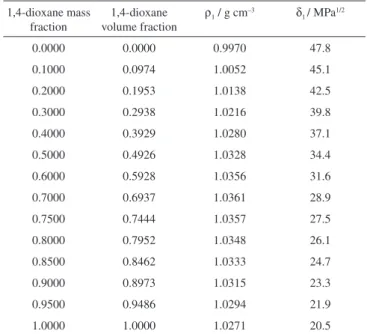
The information about polarity and volumetric behavior of 1,4-dioxane + water mixtures as a function of the composition is shown in Table 1.14 On the other hand, the calorimetric values reported in the literature for IMC were as follows, Tfus = 432.6 K and ∆Hfus = 39.46 kJ mol–1.15 From these values the calculated ideal solubility for this drug was 7.123 × 10⁻³ in mole fraction at 298.15 K.8 This value was calculated according to Equation 1.
the saturated solutions, at 298.15 K. The uncertainty in experimental solubility was lower than 1.2% from the mean. Figure 2 shows the experimental solubility and the calculated solubility by using the regular solution model (Equation 3) as a function of the solubility parameter of solvent mixtures. It is clear that experimental solubility is greater than calculated solubility probably due to strong hydrogen-bonding interactions between drug and solvents. This behavior is more evident in mixtures with δ1 lower than 32 MPa1/2.
The IMC solubility is greater in the mixture of 0.95 in mass frac-tion of 1,4-dioxane (X2 = 3.99 x 10⁻² with δ1 = 21.9 MPa1/2), but this value is slightly greater than the maximum obtained in the mixture of 0.70 in mass fraction of ethyl acetate in mixtures conformed by ethyl acetate + ethanol (X2 = 3.00 x 10⁻² with δ
1 = 20.86 MPa1/2).8 It is important to note that the maximum solubility is obtained at similar
but slightly different mixtures-solubility parameters in both binary solvent systems. Otherwise, similar but slightly different solubility values were also found in both systems. This result could be inter-preted in terms of different Lewis acid or base interactions. Besides, the main reason to obtain the maximum solubility of this drug in the mixture of 0.95 in mass fraction of 1,4-dioxane is referent to similar polarities between drug and solvent mixture in agreement with the expression “like dissolves like”.5
From density values of cosolvent mixtures and saturated solutions (Tables 1 and 2), in addition to IMC solubility (Table 2), the solvent volume fraction (φ1) and apparent molar volume of the solute (fVmol) in the saturated mixtures, were calculated. These values are also presented in Table 2.
In the literature the solute molar volume in the saturated solu-tion has been considered as a constant value when EHSA method is used.5,11 On this way, for solid compounds this property is generally calculated by means of groups’ contribution methods such as the one developed by Fedors.16 Nevertheless, this property is not independent on the solvent composition as can be see in Table 2 for apparent molar volume of IMC. This fact would be due to the different intermole-Table 1. Solvent composition in mass and volume fraction of 1,4-dioxane
(without considering IMC) in 1,4-dioxane + water mixtures, density, and Hildebrand solubility parameters at 298.15 K
1,4-dioxane mass fraction
1,4-dioxane volume fraction
ρ1 / g cm–3 δ1 / MPa1/2
0.0000 0.0000 0.9970 47.8
0.1000 0.0974 1.0052 45.1
0.2000 0.1953 1.0138 42.5
0.3000 0.2938 1.0216 39.8
0.4000 0.3929 1.0280 37.1
0.5000 0.4926 1.0328 34.4
0.6000 0.5928 1.0356 31.6
0.7000 0.6937 1.0361 28.9
0.7500 0.7444 1.0357 27.5
0.8000 0.7952 1.0348 26.1
0.8500 0.8462 1.0333 24.7
0.9000 0.8973 1.0315 23.3
0.9500 0.9486 1.0294 21.9
1.0000 1.0000 1.0271 20.5
Table 2. Hildebrand solubility parameter of mixtures, IMC solubility expressed in molarity and mole fraction, density of the saturated mixtures, apparent molar volume of IMC, solvent volume fraction in the saturated solutions, and activity coefficient of IMC expressed as decimal logarithm, at 298.15 K
δ1 / MPa1/2
IMC
ρsatd soln / g cm–3 fV
mol / cm3 mol–1 f
1 log γ2
Mol L–1 X
2
47.8 5.16×10⁻⁵ 9.32×10⁻⁷ 0.9970 358.9 1.0000 3.883
45.1 1.19×10⁻⁴ 2.32×10⁻⁶ 1.0052 355.9 1.0000 3.487
42.5 2.17×10⁻⁴ 4.60×10⁻⁶ 1.0138 352.9 0.9999 3.190
39.8 4.28×10⁻⁴ 9.92×10⁻⁶ 1.0216 350.2 0.9999 2.856
37.1 1.72×10⁻³ 4.42×10⁻⁵ 1.0280 348.0 0.9996 2.207
34.4 7.23×10⁻³ 2.10×10⁻⁴ 1.0330 315.2 0.9983 1.531
31.6 3.17×10⁻² 1.06×10⁻³ 1.0378 279.4 0.9927 0.826
28.9 0.122 4.93×10⁻³ 1.0467 261.3 0.9719 0.160
27.5 0.192 8.64×10⁻³ 1.0507 269.8 0.9559 –0.084
26.1 0.308 1.59×10⁻² 1.0549 282.6 0.9291 –0.349
24.7 0.390 2.30×10⁻² 1.0595 281.4 0.9103 –0.510
23.3 0.464 3.17×10⁻² 1.0647 277.4 0.8933 –0.648
21.9 0.502 3.99×10⁻² 1.0704 268.3 0.8846 –0.748
20.5 0.319 2.90×10⁻² 1.0551 262.8 0.9266 –0.610
cular interactions, depending on the respective solvent proportions. Nevertheless, great variability is found in the experimental fVmol values without a rational order. In particular, the great difference obtained in water-rich mixtures (greater than 315 cm3 mol–1) and those obtained in 1,4-dioxane-rich mixtures (lower than 280 cm3 mol–1) is anomalous. For these reasons, in this investigation the calculated molar volume of IMC (230.0 cm3 mol–1) was employed in the following calculations as was made with this drug in ethanol + water mixtures.8 Otherwise, no significant differences in the predictive character of EHSA were obtained in other investigations when experimental or calculated values of drug molar volumes were interchanged.7
On the other hand, according to the literature the volume fraction of the solvent mixture in the saturated solution has been calculated by means of the expression,5,11
(8)
where, V1 is the molar volume of the solvent which is calculated for solvent mixtures assuming additive volumes as,17
(9)
Nevertheless, it is well known that the mixing volumes are not additives in those mixtures with strong presence of hydrogen bonding and great differences in molar volumes. For this reason, the experi-mental solvent volume fractions were used in this investigation for all the calculations (Table 2). Solvent volume fractions were calculated by subtracting the respective drug volume contributions. The last values were calculated from molar volumes and concentrations of the drug at saturation for each cosolvent mixture.
Ultimately, the activity coefficients of IMC as decimal logarithms are also presented in Table 2. These values were calculated from ex-perimental solubility values (Table 2) and ideal solubility at 298.15 K (X2 = 7.123 × 10⁻³).8γ
2 values in water-rich mixtures were greater than unit because the experimental solubilities are lower than the ideal one.
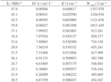
On the other hand, the parameters A, K, and W are presented in Table 3. In order to calculate the W parameter the experimental solubility parameter of IMC obtained in the mixture of 0.95 in mass fraction of 1,4-dioxane (with δ1 = 21.9 MPa1/2) was used. According with the literature, this δ2 value is the same of the solvent mixture
where the greatest drug solubility was found.5,11
As has been already indicated, the W parameter accounts for the deviations presented by real solutions with respect to regular solu-tions. These deviations are mainly due to specific interactions such as hydrogen bonding. IMC (Figure 1) and both solvents studied can establish these interactions, as hydrogen donors or acceptors because of their polar moieties, in particular due to –OH groups. 1,4-dioxane interacts just as hydrogen acceptor.
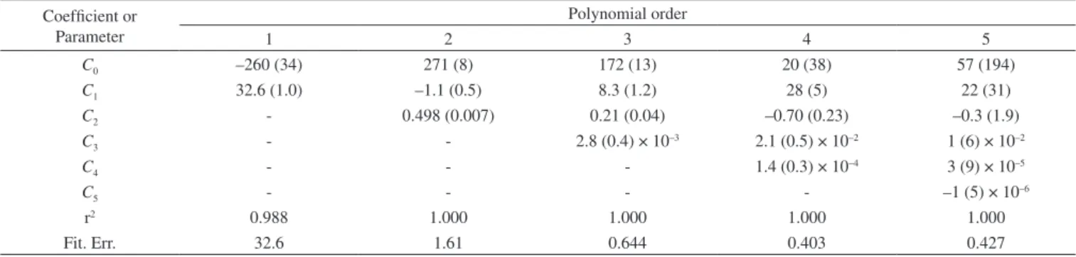
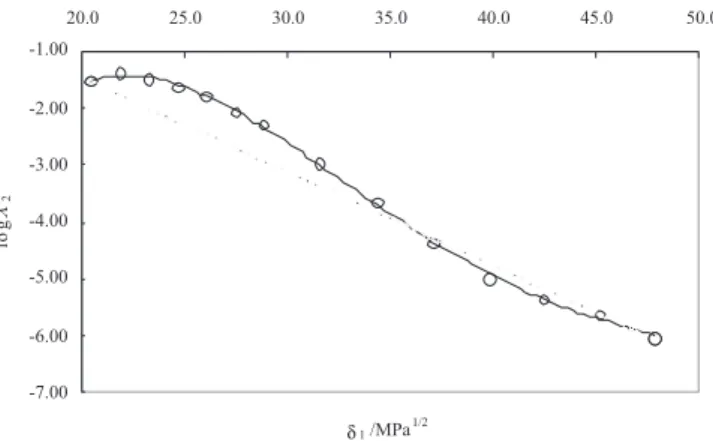
Figure 3 shows that the variation of the W parameter with respect to the solubility parameter of solvent mixtures, presents deviation from linear behavior. W values were adjusted to regular polynomials in orders from 1 to 5 (Equation 6) and their coefficients and statistical parameters are presented in the Table 4 (the empirical regressions were obtained by using MS Excel® and TableCurve 2D v5.01). The obtained W values by using the respective regular polynomials are presented in Table 5. It is clear that these values depend on the model used in the W back-calculation. Similar behaviors have been reported in the literature for several other compounds.3,7,8
Table 6 summarizes all the calculated drug solubility values. These solubilities were calculated employing the W values which were obtained by back-calculation from the polynomial models presented in Tables 4 and 5. Because we are searching the best adjust, the first criterion used to define the polynomial order of W as function of δ1 was the fitting standard uncertainties obtained, whose values were as follows, 32.6, 1.61, 0.644, 0.403, and 0.427 (Table 4), for orders 1 to 5, respectively. As another comparison criterion, Table 6 also summarizes the percentages of difference between IMC experimental solubility and those calculated by using EHSA.
According to Table 6 it follows that, as more complex the poly-nomial used is, better the agreement found between experimental and calculated solubility is. This fact is confirmed based on the mean deviation percentages (8.9 and 8.8%, for orders 4 and 5, respective-ly). In similar way to that found in other similar investigations,3,7,8 in this case, the most important increment in concordance is obtained passing from order 1 to order 2 (from 1.88 x 10⁷ to 47.8% in mean deviation). It is remarkable that mole fractions greater than unit are found between 0.40 and 0.75 in mass fraction of 1,4-dioxane by using order 1, which of course is not logic. Otherwise, significant increment in concordance is also obtained by passing from order 2 to order 3 (from 47.8 to 15.7%). Therefore, in the following calculations the model with lowest fitting uncertainty was used (order 4, Table 4).
An important consideration about the usefulness of the EHSA method is the one referent to justify the complex calculations invol-ving any other variables of the considered system (Equation 4, Tables Table 3. A, K, and W parameters for IMC in 1,4-dioxane + water mixtures
at 298.15 K
δ1 / MPa1/2 102A / cm3 J–1 K / J cm–3 a Wexpt / J cm–3 a
47.8 8.00566 0.648617 1357.970
45.1 8.00541 0.625590 1236.934
42.5 8.00505 0.603009 1121.676
39.8 8.00427 0.581498 1013.169
37.1 7.99952 0.562403 913.261
34.4 7.97924 0.545157 820.277
31.6 7.88963 0.530300 734.336
28.9 7.56219 0.518332 655.241
27.5 7.31568 0.513404 617.909
26.1 6.91153 0.509893 582.700
24.7 6.63405 0.507175 548.683
23.3 6.38883 0.505937 516.416
21.9 6.26509 0.506222 485.669
20.5 6.87359 0.506033 454.367
a 1 J cm–3 = 1 MPa
1 to 5), instead of the simple empiric regression of the experimental solubility as a function of the solvent mixtures’ solubility parameters (Table 2, Figure 4). For this reason, in the Table 7 the experimental solubilities are confronted to those calculated directly by using a regular polynomial in grade 4 of log X2 as a function of δ1 values (Equation 10, with determination coefficient r2 = 0.999 and fitting standard uncertainty = 0.054) and are also confronted to those calcu-lated involving the W parameters obtained from Equation 6 adjusted to order 4 (Table 4). The respective difference percentages are also presented in Table 7.
(10)
Based on mean deviation percentages presented in Table 7 (8.1 and 8.9% for direct calculation and EHSA method, respectively) it follows that non-significant differences are found between the values obtained by using both methods. In similar way with that found for IMC in ethyl acetate + ethanol and ethanol + water mixtures,8 the present results would be showing non-significant usefulness of EHSA method for practical purposes. The last point apparently could be controversial Table 4. Coefficients and statistical parameters for the regular polynomials of W vs. Solubility parameters of solvent mixtures free of IMC (Equation 6). Values in parentheses are the respective uncertainties
Coefficient or Parameter
Polynomial order
1 2 3 4 5
C0 –260 (34) 271 (8) 172 (13) 20 (38) 57 (194)
C1 32.6 (1.0) –1.1 (0.5) 8.3 (1.2) 28 (5) 22 (31)
C2 - 0.498 (0.007) 0.21 (0.04) –0.70 (0.23) –0.3 (1.9)
C3 - - 2.8 (0.4) × 10–3 2.1 (0.5) × 10–2 1 (6) × 10–2
C4 - - - 1.4 (0.3) × 10–4 3 (9) × 10–5
C5 - - - - –1 (5) × 10–6
r2 0.988 1.000 1.000 1.000 1.000
Fit. Err. 32.6 1.61 0.644 0.403 0.427
Table 5.W parameters (J cm–3)a back-calculated by using several polynomial
models at 298.15 K
δ1 / MPa1/2 Polynomial order
1 2 3 4 5
47.8 1297.730 1356.449 1358.718 1358.119 1358.100
45.1 1211.103 1236.318 1236.015 1236.565 1236.603
42.5 1123.965 1122.578 1121.036 1121.640 1121.650
39.8 1036.312 1015.348 1013.598 1013.760 1013.738
37.1 948.139 914.750 913.511 913.179 913.152
34.4 859.442 820.908 820.572 819.985 819.980
31.6 770.215 733.949 734.572 734.085 734.105
28.9 680.455 654.002 655.289 655.199 655.225
27.5 635.373 616.698 618.095 618.245 618.261
26.1 590.156 581.197 582.493 582.847 582.848
24.7 544.802 547.515 548.453 548.913 548.896
23.3 499.313 515.669 515.943 516.335 516.308
21.9 453.686 485.676 484.931 484.991 484.973
20.5 407.921 457.553 455.386 454.745 454.773
a 1 J cm–3 = 1 MPa
Table 6. Calculated solubility of IMC in 1,4-dioxane + water mixtures by using the W parameters obtained from regression models in orders 1, 2, 3, 4 and 5, and difference-percentages with respect to the experimental value at 298.15 K
δ1 / MPa1/2 X2 calculated % dev.a
1 2 3 4 5 1 2 3 4 5
47.8 2.11×10⁻¹⁶ 5.32×10⁻⁷ 1.23×10⁻⁶ 9.84×10⁻⁷ 9.77×10⁻⁷ 100.0 42.9 31.7 5.6 4.9
45.1 1.70×10⁻¹⁰ 1.85×10⁻⁶ 1.65×10⁻⁶ 2.02×10⁻⁶ 2.05×10⁻⁶ 100.0 20.3 28.8 12.7 11.5
42.5 1.07×10⁻⁵ 6.41×10⁻⁶ 3.63×10⁻⁶ 4.54×10⁻⁶ 4.55×10⁻⁶ 132.5 39.4 21.0 1.3 1.0
39.8 5.03×10⁻² 2.22×10⁻⁵ 1.16×10⁻⁵ 1.23×10⁻⁵ 1.22×10⁻⁵ 5.07×10+5 123.2 17.1 24.3 23.3
37.1 16.8 7.65×10⁻⁵ 4.85×10⁻⁵ 4.29×10⁻⁵ 4.25×10⁻⁵ 3.80×10+7 73.1 9.6 2.9 3.9
34.4 373 2.65×10⁻⁴ 2.34×10⁻⁴ 1.88×10⁻⁴ 1.88×10⁻⁴ 1.78×10+8 26.1 11.5 10.2 10.3
31.6 487 9.23×10⁻⁴ 1.16×10⁻³ 9.70×10⁻⁴ 9.77×10⁻⁴ 4.59×10+7 13.1 8.9 8.7 8.0
28.9 32.1 3.20×10⁻³ 5.01×10⁻³ 4.86×10⁻³ 4.90×10⁻³ 6.51×10+5 35.1 1.7 1.4 0.6
27.5 3.10 5.75×10⁻³ 9.20×10⁻³ 9.68×10⁻³ 9.73×10⁻³ 3.58×10+4 33.5 6.5 12.0 12.6
26.1 0.171 9.86×10⁻³ 1.49×10⁻² 1.67×10⁻² 1.67×10⁻² 972.9 38.0 6.4 4.8 4.8
24.7 7.04×10⁻³ 1.61×10⁻² 2.15×10⁻² 2.47×10⁻² 2.46×10⁻² 69.4 30.0 6.8 7.3 6.7
23.3 2.07×10⁻⁴ 2.54×10⁻² 2.76×10⁻² 3.09×10⁻² 3.07×10⁻² 99.3 19.7 13.0 2.4 3.1
21.9 3.92×10⁻⁶ 4.00×10⁻² 3.22×10⁻² 3.28×10⁻² 3.26×10⁻² 100.0 0.2 19.2 17.8 18.2
20.5 1.20×10⁻⁸ 7.95×10⁻² 4.01×10⁻² 3.27×10⁻² 3.30×10⁻² 100.0 174.1 38.0 12.7 13.7
Mean value b 1.88×10+7 47.8 15.7 8.9 8.8
Standard Deviation b 5.38×10+7 30.6 9.8 6.6 6.5
aCalculated as 100×|X
Table 7. Comparison of the IMC solubility values in 1,4-dioxane + water mixtures which were calculated directly and by using the EHSA
δ1 / MPa1/2 X2 % dev.a
Exptl. Calc.
direct. b
Calc. Wc
Calc. direct.
Calc. W
47.8 9.32×10⁻⁷ 1.02×10⁻⁶ 9.84×10⁻⁷ 9.1 5.6
45.1 2.32×10⁻⁶ 1.93×10⁻⁶ 2.02×10⁻⁶ 16.7 12.7
42.5 4.60×10⁻⁶ 4.38×10⁻⁶ 4.54×10⁻⁶ 4.8 1.3
39.8 9.92×10⁻⁶ 1.25×10⁻⁵ 1.23×10⁻⁵ 25.7 24.3
37.1 4.42×10⁻⁵ 4.52×10⁻⁵ 4.29×10⁻⁵ 2.2 2.9
34.4 2.10×10⁻⁴ 1.99×10⁻⁴ 1.88×10⁻⁴ 5.1 10.2
31.6 1.06×10⁻³ 9.73×10⁻⁴ 9.70×10⁻⁴ 8.4 8.7
28.9 4.93×10⁻³ 4.52×10⁻³ 4.86×10⁻³ 8.3 1.4
27.5 8.64×10⁻³ 8.97×10⁻³ 9.68×10⁻³ 3.8 12.0
26.1 1.59×10⁻² 1.62×10⁻² 1.67×10⁻² 1.6 4.8
24.7 2.30×10⁻² 2.55×10⁻² 2.47×10⁻² 10.5 7.3
23.3 3.17×10⁻² 3.37×10⁻² 3.09×10⁻² 6.4 2.4
21.9 3.99×10⁻² 3.59×10⁻² 3.28×10⁻² 10.0 17.8
20.5 2.90×10⁻² 2.92×10⁻² 3.27×10⁻² 0.7 12.7
Mean value d 8.1 8.9
Standard Deviation d 7.1 6.6
aCalculated as 100×|X
2 expt – X2 calc|/X2 expt. bCalculated using the Equation
10. cCalculated using the Equation 6 in order 4. d Calculated considering the
obtained values in the neat solvents and the twelve binary mixtures. Figure 4. Logarithmic experimental solubility of IMC as a function of the solubility parameter of the solvent mixtures at 298.15 K. Straight line corres-ponds to hypothetical logarithmic additive solubility in mixtures
considering that EHSA method implies additional experimentation including density determinations and thermal characterization of the solid-liquid equilibrium for the solid compound. Nevertheless, it is necessary keep in mind that EHSA method considers the drug solu-bility from a systematic physicochemical point of view. Moreover, it would be just necessary to found an effective method to calculate the Walker K parameter in order to calculate the W term according to the expression 2Kδ1δ2, because the δ1 and δ2 terms would be known, and thus, the drug experimental solubility could be calculated in any mix-ture in particular. Otherwise, as it was already said EHSA method has been widely employed to estimate drugs solubilities since beginning 80s of the past century and it proved to be a powerful technique in pharmaceutical sciences because it uses physicochemical properties that are easily available for several kinds of drugs.
CONCLUSION
In this investigation the EHSA method has been adequately used to study the solubility of IMC in 1,4-dioxane + water mixtures by
using calculated values of molar volume and estimated Hildebrand solubility parameter of this analgesic drug. In particular, a good predictive character has been found by using a regular polynomial in order 4 of the interaction parameter W vs. Solubility parameter of the solvent mixtures free of solute. Finally, this work expands the number of analgesic drugs successfully evaluated in front to EHSA method.
ACKNOWLEDGEMENTS
The authors thank to the DIB the Universidad Nacional de Colom-bia (UNC) for the financial support and the Department of Pharmacy of UNC for facilitating the equipments and installations used in the experimental solubility determinations.
REFERENCES
1. Budavari, S.; O’Neil, M. J.; Smith, A.; Heckelman, P. E.; Obenchain Jr., J. R.; Gallipeau, J. A. R.; D’Arecea, M. A.; The Merck Index: An Encyclopedia of Chemicals, Drugs, and Biologicals, Merck & Co., Inc.: Whitehouse Station, 13th ed., 2001; Raffa, R. B. In Remington:
The Science and Practice of Pharmacy; Gennaro, A. R., ed.; Lippincott Williams & Wilkins: Philadelphia, 21st ed., 2005.
2. Jiménez, F.; Martínez, F.; Rev. Colomb. Cienc. Quím. Farm.1995, 24, 19.
3. Martin, A.; Newburger, J.; Adjei, A.; J. Pharm. Sci.1980, 69, 659; Mar-tin, A.; Wu, P. L.; J. Pharm. Sci.1981, 72, 587; Martin, A.; Miralles, M. J.; J. Pharm. Sci.1982, 71, 439.
4. Rubino, J. T. In Encyclopedia of Pharmaceutical Technology; Swarbrick, J.; Boylan, J. C., eds.; Marcel Dekker, Inc.: New York, 1988, vol.
3, p. 375-398; Yalkowsky, S. H.; Roseman, T. J. In Techniques of
Solubilization of Drugs; Yalkowsky, S. H., ed.; Marcel Dekker, Inc.: New York, 1981, p. 91-134.
5. Martin, A.; Bustamante, P.; Chun, A. H. C.; Physical Chemical Prin-ciples in the Pharmaceutical Sciences, 4th ed., Lea & Febiger:
Philadel-phia, 1993.
6. Bustamante, P.; Romero, S.; Peña, A.; Escalera, B.; Reillo, A.; J. Pharm. Sci.1998, 87, 1590.
7. Martínez, F.; Acta Farm. Bonaerense2005, 24, 215; Martínez, F.; Rev. Acad. Colomb. Cienc.2005, 29, 429; Pacheco, D. P.; Manrique, Y. J.; Vargas, E. F.; Barbosa, H. J.; Martínez, F.; Rev. Colomb. Quím.2007, 36, 55; Aragón, D. M.; Pacheco, D. P.; Ruidiaz, M. A.; Sosnik, A. D.; Martínez, F.; Vitae, Rev. Fac. Quím. Farm.2008, 15, 113; Gantiva, M.; Martínez, F.; Quim. Nova2010, 33, 370.
8. Ruidiaz, M. A.; Martínez, F.; Rev. Colomb. Quím.2009, 38, 235; Rui-diaz, M. A.; Delgado, D. R.; Mora, C. P.; Yurquina, A.; Martínez, F.; Rev. Colomb. Cienc. Quím. Farm. 2010, 39,79.
9. Ruidiaz, M. A.; Delgado, D. R.; Martínez, F.; Marcus, Y.; Fluid Phase Equilibria2010, 299, 259.
10. Hildebrand, J. H.; Prausnitz, J. M.; Scott, R. L.; Regular and Related Solutions, van Nostrand Reinhold: New York, 1970.
11. Martin, A.; Bustamante, P.; Anal. Real Acad. Farm.1989, 55, 175. 12. The British Pharmacopoeia 1988, Her Majesty’s Stationery Office:
London, 1988, vol. I, p. 310.
13. Jiménez, J. A.; Martínez, F.; J. Braz. Chem. Soc.2006, 17, 125. 14. Ruidiaz, M. A.; Martínez, F.; Vitae, Rev. Fac. Quím. Farm.2009, 16,
327.
15. Forster, A.; Hempenstall, J.; Tucker, I.; Rades, T.; Int. J. Pharm.2001, 226, 147.
16. Fedors, R. F.; Polymer Eng. Sci.1974, 14, 147.
17. Connors, K. A.; Thermodynamics of Pharmaceutical Systems: An