The impact of forest regeneration on streamflow in 12 meso-scale humid tropical catchments

(1)

HESSD

10, 3045–3102, 2013

The impact of forest regeneration on

streamflow

H. E. Beck et al.

Title Page

Abstract Introduction

Conclusions References

Tables Figures

◭ ◮

Back Close

Full Screen / Esc

Printer-friendly Version

Interactive Discussion

Discussion

P

a

per

|

Dis

cussion

P

a

per

|

Discussion

P

a

per

|

Discussio

n

P

a

per

|

Hydrol. Earth Syst. Sci. Discuss., 10, 3045–3102, 2013 www.hydrol-earth-syst-sci-discuss.net/10/3045/2013/ doi:10.5194/hessd-10-3045-2013

Geoscientiic Geoscientiic

Hydrology and Earth System

Sciences

Open Access

Discussions

This discussion paper is/has been under review for the journal Hydrology and Earth System Sciences (HESS). Please refer to the corresponding final paper in HESS if available.

The impact of forest regeneration on

streamflow in 12 meso-scale humid

tropical catchments

H. E. Beck1, L. A. Bruijnzeel1, A. I. J. M. van Dijk2,3, T. R. McVicar2, F. N. Scatena4,*, and J. Schellekens5

1

Critical Zone Hydrology Group, Faculty of Earth and Life Sciences, VU University Amsterdam, De Boelelaan 1085, 1081 HV Amsterdam, The Netherlands

2

CSIRO Land and Water, G.P.O. Box 1666, Canberra, ACT 2601, Australia

3

Fenner School of Environment and Society, The Australian National University, Canberra, ACT 2601, Australia

4

Department of Earth and Environmental Science, University of Pennsylvania, Philadelphia, PA 19104-6316, USA

5

Inland Water Systems Unit, Deltares, P.O. Box 177, Rotterdamseweg 185, 2600 MH Delft, The Netherlands

*

deceased

Received: 19 February 2013 – Accepted: 27 February 2013 – Published: 11 March 2013

Correspondence to: H. E. Beck ([email protected])

(2)

HESSD

10, 3045–3102, 2013

streamflow

H. E. Beck et al.

Title Page

Tables Figures

◭ ◮

Back Close

Full Screen / Esc

Discussion

P

a

per

|

Dis

cussion

P

a

per

|

Discussion

P

a

per

|

Discussio

n

P

a

per

|

Abstract

Although regenerating forests make up an increasingly large portion of humid tropical landscapes, comparatively little is known of their water use and effects on streamflow (Q). Since the 1950s the island of Puerto Rico has experienced widespread aban-donment of pastures and agricultural lands, followed by forest regeneration. This paper 5

examines the possible impacts of forest regeneration on severalQmetrics for 12 meso-scale catchments (23–346 km2; mean precipitation 1720–3422 mm yr−1) with long (33– 51 yr) and simultaneous records for Q, precipitation (P), potential evapotranspiration (PET), and land cover. A simple spatially-lumped, conceptual rainfall-runoffmodel that uses dailyP and PET time series as inputs (HBV-light) was used to simulateQfor each 10

catchment. Annual time series of observed and simulated values of fourQmetrics were calculated. A least-squares trend was fitted through annual time series of the residual difference between observed and simulated time series of each Q metric. From this the total cumulative change ˆAwas calculated, representing the change in each met-ric after controlling for climate variability and water storage carry-over effects between 15

years. Negative values of ˆAwere found for most catchments andQ metrics, suggest-ing enhanced actual evapotranspiration overall followsuggest-ing forest regeneration. However, correlations between changes in urban or forest area and values of ˆA were insignifi-cant (p≥0.389) for allQ metrics. This suggests there is no convincing evidence that changes in the chosenQmetrics in these Puerto Rican catchments can be ascribed to 20

changes in urban or forest area. The present results are in line with previous studies of meso- and macro-scale (sub-)tropical catchments, which generally found no significant change in Q that can be attributed to changes in forest cover. Possible explanations for the apparent lack of a clear signal may include: errors in the land-cover, climate,Q, and/or catchment boundary data; changes in forest area occurring mainly in the less 25

(3)

HESSD

10, 3045–3102, 2013

streamflow

H. E. Beck et al.

Title Page

Tables Figures

◭ ◮

Back Close

Full Screen / Esc

Discussion

P

a

per

|

Dis

cussion

P

a

per

|

Discussion

P

a

per

|

Discussio

n

P

a

per

|

led to very different conclusions. This highlights the importance of including multiple catchments in land-cover impact analysis at the meso scale.

1 Introduction

Tropical regions have experienced extensive changes in land use and land cover dur-ing the last few decades (Lepers et al., 2005). Continuously risdur-ing demands for crop 5

land and timber have led to substantial deforestation in many regions (Drigo, 2005), and although the global tropical deforestation rate remains high at 13 Mha yr−1(FAO, 2006), forest regrowth on abandoned agricultural land is increasing, particularly in Latin America (Aide and Grau, 2004; Hecht, 2010) and South-East Asia (cf. Fox et al., 2000; Xu et al., 1999). Because these “secondary forests” account for approximately one-10

third of the total tropical forest area (Brown and Lugo, 1990; H ¨olscher et al., 2005), understanding the impact of forest regrowth on water yield is important for water re-sources management and planning purposes (Giambelluca, 2002; Bruijnzeel, 2004) and the development of viable “Payments for Ecosystem Services” schemes (Landell-Mills and Porras, 2002; Lele, 2009). However, despite this recognized importance, little 15

is known of the water use of secondary tropical forests, although there are indications of enhanced water use during the period of most active biomass accumulation (Gi-ambelluca, 2002; Juhrbandt et al., 2004; H ¨olscher et al., 2005).

The relationship between forest cover and streamflow (Q) is subject to a long-standing and ongoing discussion (Andr ´eassian, 2004), also in the tropics (Bruijnzeel, 20

2004; Calder, 2005). The influence of forest cover change on flooding is particularly contentious (e.g. FAO, 2005; Bradshaw et al., 2007; Van Dijk et al., 2009) whereas the e_ffect of forestation on tropical dry-season flows is also under debate (Calder, 2005; Scott et al., 2005). The general contention is that thenet effect of an increase in forest cover on dry-season flow depends on the “trade-off” between increases in Q due to 25

(4)

HESSD

10, 3045–3102, 2013

streamflow

H. E. Beck et al.

Title Page

Tables Figures

◭ ◮

Back Close

Full Screen / Esc

Discussion

P

a

per

|

Dis

cussion

P

a

per

|

Discussion

P

a

per

|

Discussio

n

P

a

per

|

Zimmermann et al., 2006, 2010; Hassler et al., 2011), and decreases in soil water reserves and Q on the other hand due to the higher water use of trees compared to crops, pasture, or scrubs (Bruijnzeel, 1989; Bruijnzeel, 2004; Jackson et al., 2005; Scott et al., 2005). Reviews of micro-scale (<1 km2) experimental catchment studies (e.g. Jackson et al., 2005; Brown et al., 2005) – mostly conducted outside the tropics 5

and in non-degraded settings where soil infiltration characteristics are not likely to be improved substantially by forestation – suggest that the increase in vegetation water use is indeed more important, and thus an increase in forest cover commonly leads to a decrease in both total and dry-seasonQ. However, although direct experimental ev-idence of the “infiltration trade-offhypothesis” (Bruijnzeel, 1989; Bonell et al., 2010) is 10

missing due to a lack of comprehensive studies, demonstrated reductions in amounts of headwater- or hillslope stormflow production after reforesting severely degraded land in various parts of the tropics (e.g. Chandler and Walter, 1998; Zhou et al., 2002; Zhang et al., 2004) should be large enough to overcome the associated increases in forest water use (Chandler, 2006; cf. Bruijnzeel, 2004; Scott et al., 2005; Zhou et al., 15

2010). Indeed, as long-termQ records for large, once degraded catchment areas are becoming available, evidence of improved baseflows (Qbf) following large-scale land

rehabilitation is beginning to be documented (Wilcox and Huang, 2010; Zhou et al., 2010).

The tropical island of Puerto Rico (PR) provides a solid opportunity to study the 20

impacts of natural forest regeneration on Q at the meso-catchment scale. This is as relatively high-quality long-term hydro-climatic records and sequential land-cover data are available. Since the 1950s, PR has seen widespread secondary forest regrowth on abandoned pastures, agricultural land (mostly sugar cane), and coffee plantations (Thomlinson et al., 1996; Aide et al., 2000; cf. Del Mar L ´opez et al., 1998). Although 25

(5)

HESSD

10, 3045–3102, 2013

streamflow

H. E. Beck et al.

Title Page

Tables Figures

◭ ◮

Back Close

Full Screen / Esc

Discussion

P

a

per

|

Dis

cussion

P

a

per

|

Discussion

P

a

per

|

Discussio

n

P

a

per

|

Central PR; cf. Pe ˜na-Arancibia et al., 2010). On the whole, one would expect marked drops in totalQ and Qbf during forest recovery in areas where the general extent of

soil surface degradation before land abandonment was limited and soil structural char-acteristics (and thus infiltration opportunities) therefore remained relatively unaffected by forest regeneration (cf. Aide et al., 1996; Zou and Gonzalez, 1997). For catchments 5

that experienced advanced soil degradation prior to agricultural abandonment, major declines in the volumes of both totalQ and quickflow (Qqf) would be expected during

forest regrowth due to much improved infiltration and retention capacities (cf. Chan-dler and Walter, 1998; Zhou et al., 2002). The direction and magnitude of the change inQbf will depend on the trade-offbetween the changes in vegetation water use and

10

infiltration associated with forest regeneration (Bruijnzeel, 1989; Scott et al., 2005). The following hypotheses are tested here: (1) there is a negative relationship be-tween the area under regenerating forest and the change in total Q (i.e. Qqf+Qbf);

(2)Qqf shows a negative relationship with area under regenerating forest and a

posi-tive one with area under urbanization; and (3) depending on the trade-offbetween the 15

changes in vegetation water use and infiltration associated with forest regrowth,Qbf

shows either a negative, no, or a positive relationship with the area under regener-ating forest. Specific objectives are to quantify the effects of forest regeneration and urbanization on totalQ,Qqf, andQqf.

2 Study area 20

Puerto Rico (PR) is an island with a tropical maritime climate, located in the north-eastern Caribbean occupying ∼8870 km2. The geology is dominated by the volcanic Cordillera Central, with a few major outcrops of plutonic rock (mostly granodiorite), and karstic limestones towards the far north and south (Olcott, 1999). Soils developed in the volcanic substrates are largely clayey Ultisols with a rapidly diminishing saturated 25

hydraulic conductivity (Ks) with depth (Schellekens et al., 2004) whereas the

(6)

HESSD

10, 3045–3102, 2013

streamflow

H. E. Beck et al.

Title Page

Tables Figures

◭ ◮

Back Close

Full Screen / Esc

Discussion

P

a

per

|

Dis

cussion

P

a

per

|

Discussion

P

a

per

|

Discussio

n

P

a

per

|

Island-wide mean annualP is∼1700 mm yr−1(Daly et al., 1994, 2003). There is a mod-erateP seasonality, with the three driest months of the year (January–March) receiving on average ∼1200 mm yr−1 and the three wettest months of the year (September–

November) receiving on average∼3100 mm yr−1 (Daly et al., 1994, 2003). The north-ern and eastnorth-ern portions of the island receive∼30 % more P due to the rising of the

5

moisture-bearing trade-winds against the slopes of the central mountain range (Calves-bert, 1970; Garc´ıa-Martin ´o et al., 1996; Daly et al., 2003).

During the second half of the 20th century, socio-economic changes in PR led to migration from (upland) rural areas and (lowland) ubanization (Dietz, 1986). The as-sociated abandonment of pastures and agricultural fields allowed secondary forests 10

to develop over increasingly large areas as time progressed (Thomlinson et al., 1996; Grau et al., 2003; Helmer, 2004; Par ´es-Ramos et al., 2008; Fig. 1). The dynamics of this forest recovery are well-documented, both in terms of its expansion over time, and forest composition and structure (Aide et al., 1996, 2000; Chinea and Helmer, 2003; Grau et al., 2003). Tree density typically reaches a peak between 25 and 35 years 15

after abandonment whereas species richness and forest structure resemble those of old-growth forest after ca. 40 yr of regeneration (Aide et al., 2000). Total actual evap-otranspiration (ET_a) of mature upland forest in the maritime tropical climate of PR is high compared to tropical continental sites (Schellekens et al., 2000), mostly because of enhanced wet-canopy evaporation rates (Holwerda et al., 2006, 2012), and the same 20

may well apply to the island’s secondary forests (cf. Giambelluca, 2002).

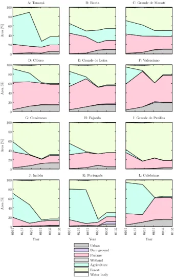
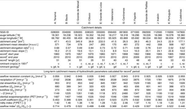
The locations of the 12 catchments examined here and the respective changes in land cover over the period 1951–2000 (see also Sect. 3.1) are shown in Fig. 1. The size of the catchments ranges from 23 to 346 km2(median size 42 km2), mean annual P varies between 1720 and 3422 mm yr−1(median value 2021 mm yr−1), and the length 25

(7)

HESSD

10, 3045–3102, 2013

streamflow

H. E. Beck et al.

Title Page

Tables Figures

◭ ◮

Back Close

Full Screen / Esc

Discussion

P

a

per

|

Dis

cussion

P

a

per

|

Discussion

P

a

per

|

Discussio

n

P

a

per

|

3 Data and methods

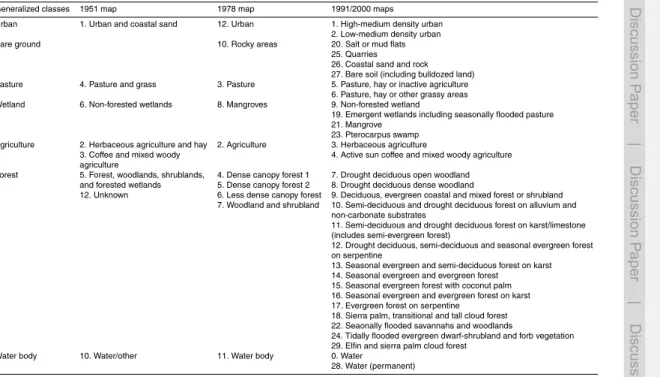
3.1 Land cover

Land-cover maps were obtained for 1951, 1978, 1991, and 2000 (Fig. 1). The maps for 1951 (Brockmann, 1952; Kennaway and Helmer, 2007) and 1978 (Ramos and Lugo, 1994) were derived from aerial photography. Although the maps for 1951 and 1978 5

were rasterized at a resolution of∼30 and ∼11 m, respectively, the actual mapping

resolution is lower due to the minimum mapping unit used by the photo interpreters. The 1991 and 2000 maps1 (∼30-m resolution; Helmer and Ruefenacht, 2005) were derived from Landsat data using regression-tree modelling and histogram matching. All land-cover maps were reprojected to a common 0.0001◦(∼11 m) geographical grid by 10

nearest-neighbour interpolation. To accommodate the different classification schemes used in the respective mapping exercises, each land-cover class was assigned to a generalized class (Table 2). For each catchment the net changes in urban and forest areas from the start of the simultaneous P, PET, and Q records (Table 1) until 2000 were calculated by linear interpolation of urban- and forest-area time series.

15

3.2 Streamflow (Q₎

All available dailyQrecords were downloaded from the US Geological Survey (USGS) National Water Information System2 in December 2012, resulting in an initial dataset of 111 gauging sites. Catchment areas were derived for each site using the PCRaster software (Wesseling et al., 1996) and the USGS National Elevation Dataset (NED) dig-20

ital elevation model (∼30-m resolution). The following criteria for inclusion here were

applied: (1) the USGS published estimate of catchment area deviated by<10 % from our computed catchment area; (2) the length of theQ record between 1950 and 2005 was >30 yr; and (3) the catchment was not subject to flow regulation or affected by

1

Downloaded from https://www.sas.upenn.edu/lczodata/ in June 2011.

2

(8)

HESSD

10, 3045–3102, 2013

streamflow

H. E. Beck et al.

Title Page

Tables Figures

◭ ◮

Back Close

Full Screen / Esc

Discussion

P

a

per

|

Dis

cussion

P

a

per

|

Discussion

P

a

per

|

Discussio

n

P

a

per

|

major anthropogenic water extraction. The latter was assessed using annual USGS Water-Data Reports3 and a map of water supply intakes in the Luquillo Experimental Forest (Crook et al., 2007; an island-wide map of intakes is lacking). The final dataset comprised 12 catchments (Fig. 1 and Table 1). For the conversion of measured dis-charge [feet3s−1] to areal meanQ [mm d−1] the computed catchment area was used. 5

The following fourQmetrics were calculated, on an annual basis, to study changes inQ through time: (1) the annual 95th percentile (percent time not-exceeded) dailyQ(Q_p95 [mm d−1]; indicative of peak flows); (2) the annual meanQ(Qtot[mm yr

−1

]; indicative of total water yield); (3) the annual 5th percentile dailyQ (Qp5 [mm d

−1

]; indicative of low flows); and (4) the annual mean dry-season (January–March) flow (Qdry[mm yr

−1

]). 10

For four catchments the daily Q strongly exceeded the daily P (see Sect. 3.5) on one or more days, indicating errors in theQand/orP data. To prevent such errors from biasing the results, for some catchments parts of the Q record were excluded from the analysis. Specifically, for the Bauta catchment data for 1996–1998 were excluded, for the Grande de Lo´ıza catchment data prior to 1961 were excluded, for the Fajardo 15

catchment data for 1989 were excluded, and for the Inab ´on catchment data for 1975 were excluded.

3.3 Precipitation (P₎

Daily P data from the Global Historical Climatology Network-Daily (GHCN-D) database4 (Gleason, 2002) and from the El Verde station in north-eastern PR5. Af-20

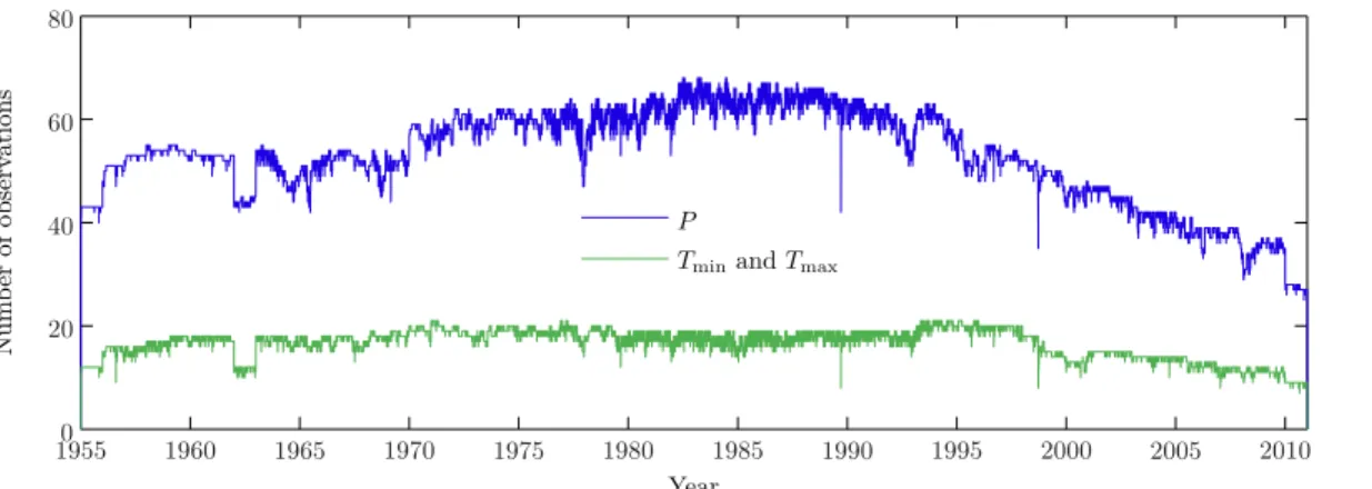
ter quality checks, The entire record from the Cerro Maravilla station (included in the GHCN-D database) and 1991–1994 data from the El Verde station were excluded from the analysis. Stations with a record>20 yr were selected from the GHCN-D database, resulting in a dataset comprising 70 stations (including the El Verde station). Figure 2

3

Available at http://wdr.water.usgs.gov/.

4

Downloaded from ftp://ftp.ncdc.noaa.gov/pub/data/ghcn/daily/ in December 2010.

5

(9)

HESSD

10, 3045–3102, 2013

streamflow

H. E. Beck et al.

Title Page

Tables Figures

◭ ◮

Back Close

Full Screen / Esc

Discussion

P

a

per

|

Dis

cussion

P

a

per

|

Discussion

P

a

per

|

Discussio

n

P

a

per

|

presents the number ofP observations available for each day between 1955 and 2010. In addition, a map6of mean annualP derived using the Precipitation-elevation Regres-sions on Independent Slopes Model (PRISM) method was used (based on data from 1963–1995; Daly et al., 1994, 2003) to ensure reliable long-term, elevation-corrected mean annualP for the catchments. The method used to obtain time series of dailyP 5

for each catchment is described in Sect. 3.5.

3.4 Potential evapotranspiration (PET)

The present study used the empirical Hargreaves equation (Hargreaves and Samani, 1985) according to guidelines set by the UN Food and Agriculture Organization (FAO; Allen et al., 1998) to assess long-term changes in the evaporative situation of the study 10

catchments. The Hargreaves equation (Hargreaves and Samani, 1985) reads:

PET=0.0023 q

Tmax−Tmin ×

_T

max+Tmin

2 +17.8

Ra, (1)

whereTminandTmaxare the daily minimum and maximum air temperature [

◦

C], respec-tively, andR_a is the extraterrestrial radiation [mm d−1].R_awas computed as described by Allen et al. (1998).

15

The choice for the empirical Hargreaves method was motivated on the one hand by the lack of available long-term data for the climatic variables required for more phys-ically based methods such as the Penman-Monteith equation (Monteith, 1965), and on the other hand by the better availability ofTmin and Tmax data. Daily Tmin and Tmax

time series (>20 yr) are available for 21 stations in PR within the GHCN-D database 20

(Gleason, 2002). Figure 2 presents the number of dailyT_minandT_maxobservations be-tween 1955 and 2010. Maps of mean annualTminandTmaxfrom the WorldClim dataset

7

6

Downloaded from http://www.wcc.nrcs.usda.gov/ftpref/support/climate/prism/ in Septem-ber 2011.

7

(10)

HESSD

10, 3045–3102, 2013

streamflow

H. E. Beck et al.

Title Page

Tables Figures

◭ ◮

Back Close

Full Screen / Esc

Discussion

P

a

per

|

Dis

cussion

P

a

per

|

Discussion

P

a

per

|

Discussio

n

P

a

per

|

(∼1-km resolution; Hijmans et al., 2005) were also used to ensure reliable mean

an-nual values. The approach followed to obtain catchment-wide daily mean time series ofTmin andTmax is outlined in Sect. 3.5. The Hargreaves method has been evaluated

successfully against PET based on the Penman–Monteith equation (Trajkovic, 2007) and various other equations (Lu et al., 2005; Sperna Weiland et al., 2012).

5

3.5 Spatio-temporal interpolation and rescaling of climatic variables

To calculate catchment-wide daily mean time series of the climatic variablesP, Tmin,

andTmax from 1955 (marking the start of many records) to 2010 an approach was

de-veloped that: (1) removed the linear trend from the time series for each station and variable; (2) spatially interpolated the trend and daily-irregular components; and (3) re-10

united them on a per-pixel basis; after which (4) the time series were rescaled. More specifically, the following steps were carried out for each variable (where X denotes the variable in question):

1. Tmin and Tmax data were converted from

◦

C to K. For each station with record length>20 yr trends were calculated from annual meanX time series using the 15

non-parametric Mann–Kendall statistical test (Kendall, 1975; Mann, 1945) with Sen’s estimate of slope (Sen, 1968).

2. For each station daily X time series were de-trended and divided by the station mean such that the new mean is unity.

3. Daily maps with a resolution of 0.02◦ (∼2 km) were computed from time series 20

ofX trend (having a constant value for each station) and from time series of de-trended unityX values using spatial interpolation (see next paragraph).

4. On a per-pixel basis the cumulative integral of the trend was calculated and offset such that the mean is unity, resulting in time series of netX change.

5. By multiplying the time series of netX change by time series of de-trended unity 25

(11)

HESSD

10, 3045–3102, 2013

streamflow

H. E. Beck et al.

Title Page

Tables Figures

◭ ◮

Back Close

Full Screen / Esc

Discussion

P

a

per

|

Dis

cussion

P

a

per

|

Discussion

P

a

per

|

Discussio

n

P

a

per

|

6. The time series of unity X values were multiplied times a map of elevation-corrected long-term meanX (PRISM forP, and WorldClim forTmin andTmax; see

Sects. 3.3 and 3.4, respectively).

7. Finally, dailyX time series were calculated for each catchment by averaging over all the pixels comprising each catchment, and theTmin andTmaxtime series were

5

re-converted from K to◦C.

The most common techniques used for spatial interpolation (Hartkamp et al., 1999) are Thiessen polygons (Thiessen, 1911), inverse-distance weighting (IDW; Shepard, 1968; Dirks et al., 1998), kriging (Krige, 1951), and splining (Tait et al., 2006). Given the large number of maps that required interpolation, here we employed the computa-10

tionally efficient IDW technique. IDW computes a value at an unsampled location (X0)

from the weighted neighbourhood observations (Xj) as follows:

X0 = R P

j=1

X_jv_j

R P

j=1

v_j

, (2)

where j denotes the j-th observation, v_j are the weights given to neighbouring ob-servations, while the summation is overj=1, 2, ...,R. The weights were calculated 15

according to:

v_j = 1

gc_j , (3)

where g_j is the distance between X_j and X0, and the exponent c determines the

(12)

HESSD

10, 3045–3102, 2013

streamflow

H. E. Beck et al.

Title Page

Tables Figures

◭ ◮

Back Close

Full Screen / Esc

Discussion

P

a

per

|

Dis

cussion

P

a

per

|

Discussion

P

a

per

|

Discussio

n

P

a

per

|

2007), following recommendations by Garcia et al. (2008), and to reduce computational time, here a constant value of 3 forcwas assumed.

The present approach has two advantages over the customary approach of using the nearest station with the longest record. Firstly, information from all nearby stations with records>20 yr is incorporated. Secondly, our approach ensures unbiased mean 5

annual values by rescaling against elevation-corrected long-term means. On the other hand, there are two caveats. First of all, portions of a time series may originate from dif-ferent stations, thereby introducing spurious signals if, for instance, they have different seasonal patterns. Furthermore, for P, step six of the approach merely changes the intensity of the series, and does not correct for storm events unsampled by the isolated 10

“point” network of meteorological stations.

3.6 HBV-light model

The HBV-light model (Seibert, 2005) was used to simulateQ. HBV-light is a spatially-lumped, conceptual rainfall-runoffmodel based on the HBV model (Bergstr ¨om, 1976). HBV-light runs at a daily time step, has two groundwater stores and one unsaturated-15

zone store, and uses daily time series ofP, PET, andT as inputs. T was not relevant in the present case since it is only used to drive the snow model subroutine. Rainfall interception is not estimated explicitly in HBV-light but is implicit in the BETA, FC, and UZL parameters. Although the model has been used predominantly in temperate-zone catchments (e.g. te Linde et al., 2008; Steele-Dunne et al., 2008; Driessen et al., 2010), 20

it has also been used successfully in tropical settings and for a range of catchment sizes, e.g. in Fiji (0.63 km2; Waterloo et al., 2007), Southern Ecuador (75 km2; Plesca et al., 2012), and Thailand (12 100 km2; Wilk et al., 2001). For in-depth discussion of the model, see Seibert (2005). Table 3 briefly describes the model parameters and lists the calibration ranges used. We were unable to close the water balance for sev-25

(13)

HESSD

10, 3045–3102, 2013

streamflow

H. E. Beck et al.

Title Page

Tables Figures

◭ ◮

Back Close

Full Screen / Esc

Discussion

P

a

per

|

Dis

cussion

P

a

per

|

Discussion

P

a

per

|

Discussio

n

P

a

per

|

parameter (PCORR) was introduced that scaledP as required to match observed and predictedQ. The influence of theP scaling on the model’s results is limited because the simulatedQwas only used to control for climate and storage carry-over effects (see Sect. 3.7).

Model parameters for each catchment were calibrated using Latin hypercube sam-5

pling (LHS; McKay et al., 1979). LHS is a more efficient alternative (Yu et al., 2001) to the commonly used Monte Carlo technique (Metropolis, 1987; Beven, 1993; Seibert, 1999). Using LHS the parameter space (Table 3) is split up innequal intervals. Values for the parameters are generated by sampling each interval just once in a random man-ner. The model is runntimes with random combinations of the parameter values from 10

each interval for each parameter. Here n=30 000 model runs were used to ensure convergence of the performance criterion. The first 10 yr of the record (Table 1) were used as spin-up period to initialize the groundwater stores after which the model was run for the entire period (i.e. the first 10 yr were run twice). The split-sample procedure (Refsgaard, 1997) was used to calibrate the parameters against data from the second 15

half of the period and validate the parameters against data from the first half of the period.

Parameters of hydrological models are commonly calibrated using a composite of objective functions (i.e. a summary statistic incorporating several measures of perfor-mance; e.g. Madsen, 2000). Here, three di_fferent objective functions that strike a bal-20

ance between accurate representations of all portions of the hydrograph were used. The first objective function represents the Nash-Sutcliffe efficiency (Nash and Sutcliffe, 1970; NS [−]). The NS is defined as:

NS₌1−

k P

t=1

Qto−Q t s

2

k P

t=1

Qot −Qo

2

(14)

HESSD

10, 3045–3102, 2013

streamflow

H. E. Beck et al.

Title Page

Tables Figures

◭ ◮

Back Close

Full Screen / Esc

Discussion

P

a

per

|

Dis

cussion

P

a

per

|

Discussion

P

a

per

|

Discussio

n

P

a

per

|

where Qs and Qo represent 3-D mean simulated and observed Q, respectively

[mm d−1], t is the time step [−], and the summation is over t₌1, 2, ..., k. The

sec-ond objective function (NSlog [−]) is the NS calculated from log-transformed Qs and Qo, thereby giving more weight to low Q values. NS and NSlog were calculated from

3-D meanQto account for the flashy nature of the streams, which resulted in frequent 5

mismatches between daily peaks of observed and simulatedQ, thereby confounding the calibration. The third and final objective function represents the volume error (VE [%]):

VE=100Qs−Qo Qo

. (5)

For each run, the objective functions were combined to form a single score using the 10

combined-rank method (Booij and Krol, 2010).

The main analysis was conducted using the 30 “best”Qsimulations. Parameter un-certainty (e.g. Beven, 1993; Seibert, 1997) was quantified as described in Sect. 3.7. It should be noted that the K2 parameter in HBV-light was not calibrated, but was set to 1−k_bf(wherekbf is the baseflow recession constant listed in Table 1). In addition, the

15

MAXBAS parameter was not calibrated, but was set to one, since the travel time for the catchments under study is likely to be less than a day (confirmed by exploratory cali-bration efforts in all catchments). The PCORR parameter was calibrated only for catch-ments that had absolute VE values>20 % for the calibration period when PCORR was set to one and parameter combinations were exhausted. For these catchments, the 20

(15)

HESSD

10, 3045–3102, 2013

streamflow

H. E. Beck et al.

Title Page

Tables Figures

◭ ◮

Back Close

Full Screen / Esc

Discussion

P

a

per

|

Dis

cussion

P

a

per

|

Discussion

P

a

per

|

Discussio

n

P

a

per

|

3.7 Evaluation of the impacts of land-cover change on streamflows

For each catchment and Q metric, annual time series of the observations and the 30 best simulations were calculated, and annual time series of the deviations D be-tween the two were calculated as:

D_dx =100Q x

obs −Q

x sim,d Qx_obs

, (6)

5

where D are the deviation time series [%], Qobs and Qsim are annual time series of

the observed and simulated Q metrics [mm yr−1], respectively, x is the year [−], and d=1, 2, ..., 30 are the simulations. D integrates the e_ffects ofP and PET variability and basin carry-over storage on the Q metrics, thereby isolating the impact of other factors, notably land-cover change.

10

For each catchment and Q metric, trend lines were fitted through time series of D prior to 2000, expressed by the following equation:

y =a x+b, (7)

wherey is the trend line [%] andaandbare fitted parameters [%]. The parameterais the slope of the trend, indicating the change inD prior to 2000, when land-cover data 15

is available. For each catchment andQmetric, the estimated value ofa(termed ˆaJ[%])

and the associated standard error (termed ˆσJ [%]) were calculated from the annual

time series of deviation D using the non-parametric jackknife resampling technique (Quenouille, 1956; Tukey, 1958). From each annual time series ofD consisting of M values, this procedure takesMsubsamples ofM−1 values by omitting a different value 20

each time. The parameter values of Eq. (7) are re-computed for each subsample, using the least-squares method, thus obtaining for eachQmetric a 30-by-M matrix ofaand b estimates. The mean of the a estimates is the jackknife-estimated value of a ( ˆaJ).

The total change ( ˆA[%]) inDprior to 2000 is calculated by: ˆ

A=aˆJL, (8)

(16)

HESSD

10, 3045–3102, 2013

streamflow

H. E. Beck et al.

Title Page

Tables Figures

◭ ◮

Back Close

Full Screen / Esc

Discussion

P

a

per

|

Dis

cussion

P

a

per

|

Discussion

P

a

per

|

Discussio

n

P

a

per

|

whereL [−] is the length of the record until 2000 (cf. Table 1). ˆA can be interpreted as the cumulative residual change in annual observed values of the Q metric after accounting for the effects of climate variability and carry-over water storage on theQ metric.

The standard error of ˆaJconsists of two parts. The first ( ˆσs[%]) was calculated from

5

the mean dispersion of ˆa within the time series ofD, and is indicative of observational errors in P, PET, and Q data, possible defects in the HBV-light model structure, and faulty assumptions in the formulation of Eq. (7). ˆσs was calculated using the jackknife

technique as follows:

ˆ σs =

1 30

30

X

d=1

v u u

tM

−1 M

M X

i=1

ˆ

a_{d i} −aˆ_d2, (9)

10

where ˆa_{d i} [%] are the estimates of a for subsamples i=1, 2, ...,M of annualD time seriesd=1, 2, ..., 30. The second part of the standard error ( ˆσp [%]) was calculated

from the dispersion of the mean a amongst the 30 time series of D, and is mainly indicative of parameter uncertainty. It was calculated as:

ˆ

σp =std

ˆ

a_d₌1, ˆad=2, ..., ˆad=30

, (10)

15

where std refers to the standard deviation. The two parts were combined to yield the standard error of ˆaJ ( ˆσJ[%]) as follows:

ˆ

σJ =σˆs+σˆp. (11)

The standard error associated with ˆA( ˆσ_Aˆ[%]) is given by:

ˆ

σ_Aˆ =σˆJL. (12)

20

(17)

HESSD

10, 3045–3102, 2013

streamflow

H. E. Beck et al.

Title Page

Tables Figures

◭ ◮

Back Close

Full Screen / Esc

Discussion

P

a

per

|

Dis

cussion

P

a

per

|

Discussion

P

a

per

|

Discussio

n

P

a

per

|

in forest or urban area per catchment and corresponding values of ˆA. Conventionally a significance level of 0.05 is applied, but this level was adjusted for the number of infer-ences made (four in the present study) to 0.01 using the Bonferroni procedure (Bland and Altman, 1995).

4 Results 5

4.1 Changes in climatic variables

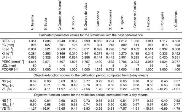
Using the new P dataset (1955–2010), which comprises the records from 70 sta-tions, per-pixel trends for the island ranging from−0.25 to +0.41 % yr−1 (mean value

+0.02 % yr−1) were found (Fig. 3a). In addition, a strong north-south disparity was ob-served, with positiveP trends mainly identified to the south of the Cordillera Central, 10

and negative trends north of it (Fig. 3a). Likewise, the new PET dataset (1955–2010), based on 21 stations, shows similar magnitudes of change, with per-pixel values rang-ing from−0.30 to+0.17 % yr−1(mean value−0.03 % yr−1), but with a less clear spatial pattern compared toP (Fig. 3b).

4.2 HBV-light model performance 15

Table 4 lists the calibrated parameter values for the HBV-light model plus objective function scores for the calibration and validation periods for each catchment. Median Nash-Sutcliffe (NS) values of 0.64 and 0.63 (median of 12 values, where each value represents the mean NS value of the 30 best simulations for each catchment) were obtained for the calibration and validation periods, respectively (Table 4). The median 20

(18)

HESSD

10, 3045–3102, 2013

streamflow

H. E. Beck et al.

Title Page

Tables Figures

◭ ◮

Back Close

Full Screen / Esc

Discussion

P

a

per

|

Dis

cussion

P

a

per

|

Discussion

P

a

per

|

Discussio

n

P

a

per

|

catchments required optimization of the PCORR parameter (cf. Table 4), possibly due to biases in the PRISMP map,Q and/or catchment boundary data, water extractions, and/or inter-basin groundwater transfers, which combined may cancel out or amplify one another.

4.3 Changes in land cover 5

Figure 4 shows the land-cover time series for each catchment. In all catchments forest and urban areas increased markedly between 1951 and 2000 at the expense of pasture and agricultural areas. During the period of simultaneous P, PET, and Q recording (Table 1) the net change in forest and urban areas for the study catchments ranged from +2 to +55 % (mean value +26 %) and from +2 to +11 % (mean value +7 %), 10

respectively. The changes in pasture and agricultural areas ranged from−19 to+26 %

(mean value−7 %) and from−63 to+9 % (mean value−26 %), respectively.

4.4 Changes in streamflow metrics

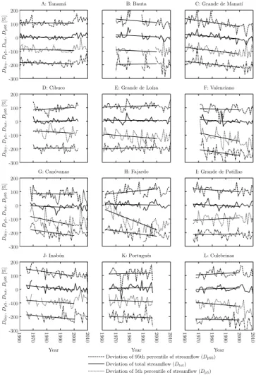
For each catchment and Q metric, Fig. 5 shows annual time series of the difference between observed and simulatedQas expressed byD(Eq. 6) and the corresponding 15

fitted trend lines (y in Eq. 7), whereas Table 5 lists values of the total change ˆA(Eq. 8) and the corresponding error ˆσ_Aˆ (Eq. 12). Catchments with low NS values generally

gave higher ˆσ_Aˆ values (cf. Tables 4 and 5). In general D_tot shows the least temporal

variability (Fig. 5), which is reflected by low ˆσ_Aˆvalues for ˆAtot (Table 5). The low

tempo-ral variability ofQtot is likely due to the low degree of sampling error associated with the

20

calculation of annual meanQ. Most catchments show progressive decreases over time in their time series ofD(Fig. 5), as indicated by the mostly negative ˆAvalues (Table 5), suggesting decreases in observed Q metrics that are unrelated to carry-over effects of water storage and climate variability. The most pronounced decreases inQ_tot were found for catchments B, C, and J, whereas a moderate increase was found for catch-25

(19)

HESSD

10, 3045–3102, 2013

streamflow

H. E. Beck et al.

Title Page

Tables Figures

◭ ◮

Back Close

Full Screen / Esc

Discussion

P

a

per

|

Dis

cussion

P

a

per

|

Discussion

P

a

per

|

Discussio

n

P

a

per

|

were found for catchments A, C, F, G, H, J, K, and L, whereas a (moderate) increase was found only for catchment I. Clear decreases in theQmetric related to peak flows (Qp95) were found for catchments B, C, I, and J, whereas strong increases were found

for catchments D, H, and L.

4.5 Impacts of land-cover change on streamflows 5

Figure 6 shows regressions between the amount of urban and forest area change vs. the cumulative change in annual time series of D prior to 2000 (expressed by ˆA in Eq. 8) for each Q metric. In spite of strong increases in forest and urban area, and pronounced changes inD over time for theQ metrics of several catchments, all correlations were insignificant (p≥0.389). Nonetheless, a weak (i.e. non-significant) 10

positive relationship can be observed between changes in forest cover and changes in annual total streamflowQ_tot, when excluding catchments C and J (which appear to be outliers; Fig. 6c).

5 Discussion

5.1 Changes in climatic variables 15

Previous research on long-term changes inP in PR, mostly using a limited number of climate stations, has suggested progressive declines in long-termP over 1900–2000 (Larsen, 2000; Van der Molen, 2002), but to the authors’ knowledge no comprehensive analysis has been conducted for the entire island. Using the new P dataset (1955– 2010) a strong north-south disparity in terms of trend was observed (Fig. 3a), which 20

may be attributed to changes in wind patterns induced in turn by changes in sea sur-face temperature (Comarazamy and Gonz ´alez, 2011; cf. Van der Molen et al., 2006). Although trends in PET (1955–2010) were just as strong, they showed a less clear spatial pattern. Nevertheless, these findings reaffirm the importance of accounting for climate variability in studies assessing the e_ffects of land-cover changes onQ.

(20)

HESSD

10, 3045–3102, 2013

streamflow

H. E. Beck et al.

Title Page

Tables Figures

◭ ◮

Back Close

Full Screen / Esc

Discussion

P

a

per

|

Dis

cussion

P

a

per

|

Discussion

P

a

per

|

Discussio

n

P

a

per

|

5.2 Impacts of land-cover change on streamflows

We were unable to accept the three hypotheses because no significant relationships (p <0.01) were found between the change in forest cover or urban area, and the change in the investigated Q metrics across the 12 catchments (Fig. 6). This result agrees with previous meso- to macro-scale catchment studies in the tropics, subtrop-5

ics, and warm-temperate regions (Table 6), which mostly failed to demonstrate a clear relationship between Q and change in forest area. Our use of multiple catchments proved important since many individual catchments showed pronounced changes in flow characteristics that might well have been attributed to land-cover change other-wise.

10

Nevertheless, a weak positive relationship was observed between the change in forest cover and the change inQtot (Fig. 6c), tentatively suggesting that regeneration

of forests leads to increases in Q in PR. If true, this would imply that in the investi-gated catchments the increase in Q due to enhanced rainfall infiltration during forest regrowth overrides the decrease in Q associated with the greater water use of the 15

aggrading forests (cf. Bruijnzeel, 1989; Scott et al., 2005). The soils beneath young secondary forests in PR show higher bulk density than beneath mature secondary forests (Weaver et al., 1987; Lugo and Scatena, 1995) and are less structured (Lugo and Helmer, 2004). Presumably, this reflects soil compaction by livestock and cropping prior to abandonment and subsequent secondary forest regeneration. However, the 20

general level of soil degradation under pasture in PR (cf. Aide et al., 1996) is proba-bly not sufficient to cause widespread occurrence of overland flow, although surface erosion under sugar cane and coffee plantations has been reported to be rampant in parts of the island (e.g. Del Mar L ´opez et al., 1998; Smith and Abru ˜na, 1955). Un-fortunately, to date, no unequivocal case of a positive relationship between changes 25

(21)

HESSD

10, 3045–3102, 2013

streamflow

H. E. Beck et al.

Title Page

Tables Figures

◭ ◮

Back Close

Full Screen / Esc

Discussion

P

a

per

|

Dis

cussion

P

a

per

|

Discussion

P

a

per

|

Discussio

n

P

a

per

|

et al., 2002; Zhang et al., 2004; Sun et al., 2006) must be considered large enough to overcome the associated increases in forest water use (Chandler, 2006; cf. Brui-jnzeel, 2004; Scott et al., 2005). Nevertheless, long-term streamflow data for large, once degraded but subsequently rehabilitated catchments in sub-humid Texas (Wilcox and Huang, 2010) and the humid Red Soils region of South China (Zhou et al., 2010) 5

have recently indicated gradually increasedQbf over prolonged periods of time

follow-ing large-scale land rehabilitation and regreenfollow-ing, suggestfollow-ing soil improvement to be the dominant factor in these cases. Further process-based work is required to sub-stantiate this contention. Similarly, pending the results of hydrological process studies in PR’s regenerating forests (in particular, infiltration and soil water retention vs. forest 10

water use) the presently obtained apparent positive relationships between the change in forest cover and the change inQtot may be spurious.

The present investigation is confounded somewhat by modest urbanization occur-ring simultaneously with forest regeneration in some of the investigated catchments (Fig. 4). Since urbanization typically increases the area of impervious surfaces, thereby 15

enhancing the frequency and intensity of infiltration-excess overland flow, moreQqfis

produced (e.g. Harto et al., 1998; DeWalle et al., 2000; Ziegler et al., 2004; Rijsdijk et al., 2007). This, if progressing beyond a critical threshold, can even result in re-ductions in Qbf (Van der Weert, 1994; Bruijnzeel, 1989; Bruijnzeel, 2004) on top of

the reductions incurred already by the higher water use of the regenerating forest (Gi-20

ambelluca, 2002). However, no significant relationships (p <0.01) between the degree of urbanization and changes in any of the observedQmetrics in our catchments were identified (Fig. 6). This is probably due to insu_fficient amounts of urbanization occurring (+2 to+11 %, mean value of+7 %; Fig. 4). Similarly, studies of the “flashiness” (sensu Baker et al., 2007) of the runoffbehaviour of urbanized and forested catchments in PR 25

revealed no di_fferences (Ram´_ırez et al., 2009; Phillips and Scatena, 2010). However, Phillips and Scatena (2010) did detect significant differences (p <0.05) in the frequency of stage change (cf. McMahon et al., 2003), possibly indicating locally enhancedQqf

(22)

HESSD

10, 3045–3102, 2013

streamflow

H. E. Beck et al.

Title Page

Tables Figures

◭ ◮

Back Close

Full Screen / Esc

Discussion

P

a

per

|

Dis

cussion

P

a

per

|

Discussion

P

a

per

|

Discussio

n

P

a

per

|

Wu et al. (2007) reported a change in Qtot of −25 % (corrected for changes in P

using a single P station that was not included in the current study as it did not meet the necessary quality requirements), between 1973–1980 and 1988–1995 for the R´ıo Fajardo catchment in north-eastern PR (here identified as catchment H). Wu et al. (2007) attributed this negative change inQto the small amount of forest regeneration 5

occurring during that period (estimated at 8 % based on the interpolated time series shown in Fig. 4). For the same catchment, here a similar change in Qtot of −31 %

(calculated usingDtot) was found between the respective periods. However, a much

smaller estimated change of (−5±4) % was obtained between the respective periods when taking into account the complete record (48 yr), using the calculated trend inDtot

10

prior to 2000 ( ˆaJ) and the corresponding standard error ( ˆσJ, Eq. 11). Thus, Wu et al.

(2007) may have overestimated the reduction in Qtot for the R´ıo Fajardo catchment

because they only used part of the available record. Additionally, given that the R´ıo Fajardo catchment appears to be an outlier in the present analysis (Figs. 6e and 6f), possibly due to non-quantified anthropogenic water extractions, any inferences for this 15

catchment should be viewed with caution.

5.3 Field-based estimates of vegetation water use

To explore the possible changes in total water yield that may be associated with a conversion from shaded coffee, sugar cane or pasture (the dominant land uses in PR in 1951, see Sect. 3.1) to (semi-)mature secondary forest (current situation), it 20

is of interest to compare the typical amounts of total water use (ET_a) by the respec-tive vegetation types. Field-based estimates of transpiration plus soil evaporation for shaded coffee and sugar cane in PR range between, respectively, 1.4–3.2 mm d−1(Lin, 2010; Guti érrez and Meinzer, 1994) and 2.5–4.6 mm d−1 (V ázquez, 1970; Fuhriman and Smith, 1951; Goyal and Gonz ález-Fuentes, 1989; cf. Harmsen, 2003). The mean 25

(23)

HESSD

10, 3045–3102, 2013

streamflow

H. E. Beck et al.

Title Page

Tables Figures

◭ ◮

Back Close

Full Screen / Esc

Discussion

P

a

per

|

Dis

cussion

P

a

per

|

Discussion

P

a

per

|

Discussio

n

P

a

per

|

2006). Thus, despite the deeper root systems of the forests (cf. Nepstad et al., 1994), mean soil water use for the agricultural crops under consideration, pasture, and forests is quite similar, possibly due to the relatively rainy climate prevailing in PR all year round (Calvesbert, 1970). To this, rainfall interception losses (higher for forest) should be added. The best estimates of rainfall interception for mature Tabonuco forest (∼21 %

5

of mean annualP; Holwerda et al., 2006) translate to ca. 1.2 mm d−1 for an annualP of 2000 mm yr−1 (i.e. the approximate average rainfall for the 12 study catchments), vs. 0.9 mm d−1 for shaded co_ffee (Siles et al., 2010) and 0.2 mm d−1 for sugar cane (Leopoldo et al., 1981). Extrapolating the above-mentioned average values to a year, gives mean estimated ETatotals for shaded coffee, sugar cane, and pasture of,

respec-10

tively, ca. 1170, 1355, and 1020 mm yr−1vs. ca. 1515 mm yr−1for mature forest. Thus, the full conversion from pasture or crop land to mature forest could potentially change Qtot by about −160 mm yr

−1

(in the case of sugar cane) to−495 mm yr−1 (in the case

of pasture).

For the catchments examined here a mean modeled change inQtot of−86 mm yr

−1

15

(standard deviation±124 mm yr−1) was found (calculated from values of ˆA_tot and Q_tot

listed in Tables 5 and 1, respectively). If it is assumed that this change was solely due to the mean change in forest cover of +26 %, the full conversion from pasture or crop to mature secondary forest would have resulted in a change in Qtot of about

(−340±480) mm yr−1. Although the modeled change inQ_tot lies in between the above

20

estimates based on local field studies of ETa, the very high standard deviation of the

estimated modeled change inQtot suggests that this agreement may be mere chance.

Therefore, the question re-emerges as to why analysis of the impacts of land-cover change onQin meso-scale tropical catchments does not confirm the findings of micro-scale experimental studies, which clearly demonstrate a relationship between change 25

(24)

HESSD

10, 3045–3102, 2013

streamflow

H. E. Beck et al.

Title Page

Tables Figures

◭ ◮

Back Close

Full Screen / Esc

Discussion

P

a

per

|

Dis

cussion

P

a

per

|

Discussion

P

a

per

|

Discussio

n

P

a

per

|

5.4 Potential explanations for the lack of relationships

Upscaling in hydrology is an outstanding issue that has received considerable atten-tion (e.g. Peterson, 2000; Rodriguez-Iturbe, 2000; McDonnell et al., 2007; Bl ¨oschl and Montanari, 2010). For many studies the lack of a clear relationship between deforesta-tion and change in Q can be explained by the rapid regeneration of tropical forests, 5

where ETaquickly reverts back to its original level and possibly exceeds it for decades

(Giambelluca, 2002; Bruijnzeel, 2004; Juhrbandt et al., 2004). However, this expla-nation does not apply to the present study, since the catchments were exploited as pastures or agricultural fields for a sustained period of time prior to their abandonment and subsequent forest regeneration. Another possible reason for the inconclusive re-10

sults obtained by many studies is the use of seasonal or annual meanQ metrics only, whereas it is generally preferred to use metrics related to the frequency and magnitude ofQ(Alila et al., 2009, 2010), particularly when evaluating the change in peak flows. Finally, the failure to correct for climatic variability by many studies may also have led to inconclusive, or even erroneous, outcomes.

15

The first among the potential explanations for the lack of relationship between land-cover change andQ metrics in PR is covariance between land cover and climate in space, due to landscape ecology and history (cf. Van Dijk et al., 2012), or in time, due to land-cover changes altering the climate (Van der Molen, 2002; Pielke et al., 2007). Several meso-scale atmospheric modelling studies have produced conflicting results 20

regarding the existence of such a relationship for PR (Van der Molen et al., 2006; Co-marazamy and Gonz ´alez, 2011). The contrastingP trends reported here for different parts of the island (Fig. 3a) are also unable to provide evidence since similar magni-tudes of forest regeneration occur across the island (Fig. 1). Also, because observed P and PET time series were input to the HBV-light model, most of the covariance 25

(25)

HESSD

10, 3045–3102, 2013

streamflow

H. E. Beck et al.

Title Page

Tables Figures

◭ ◮

Back Close

Full Screen / Esc

Discussion

P

a

per

|

Dis

cussion

P

a

per

|

Discussion

P

a

per

|

Discussio

n

P

a

per

|

A second potential explanation is that the land-cover, P, PET, Q, and catchment boundary data used here contain more errors than those used in small, commonly well instrumented, experimental studies. Using data for 278 Australian catchments Van Dijk et al. (2012) showed that the introduction of noise to long-term means of observed PET,P, andQreduced the likelihood of detecting a land-cover signal. Here, as diff er-5

ent methodologies were employed to derive the land-cover maps for the different years, and because the maps had different spatial resolutions and classification schemes (see Sect. 3.1), it is conceivable that the land-cover time series contained errors. ForP a higher station density is probably desirable, particularly in tropical areas where the uncertainty in estimated catchment-wideP is exacerbated by the predominantly con-10

vective character ofP and the limited spatial extent of individual storm cells (Nieuwolt, 1977; Hastenrath, 1991). Likewise, the PET data should also be viewed with caution, since net radiation, wind speed, and relative humidity, other dominant factors control-ling PET magnitude and trends (see McVicar et al., 2012, and references therein), were not explicitly included in its calculation (cf. Eq. 1). The error in the PRQdata is 15

about 3–6 % (Sauer and Meyer, 1992). The cumulative error in annualP, PET, andQ was quantified by ˆσ_Aˆ (Eq. 12). Even though ˆσ_Aˆ does not account for the error in the

land-cover data or for drift errors in theP, PET, and/orQdata during the study period, values of ˆσ_Aˆ already constitute a substantial portion of the variance in ˆAvalues (the

estimated total change in the observed Q) for all Q metrics (cf. Table 5, and Fig. 6). 20

This suggests that errors in land-cover,P, PET, andQdata may have restricted the de-tection of a relationship between land-cover change andQmetrics in PR. Kundzewicz and Robson (2004) and Chappell and Tych (2012) also suggested that a high degree of observational error may mask the identification ofQchange.

A third potential explanation is that the amount of forest area change in the inves-25

(26)

HESSD

10, 3045–3102, 2013

streamflow

H. E. Beck et al.

Title Page

Tables Figures

◭ ◮

Back Close

Full Screen / Esc

Discussion

P

a

per

|

Dis

cussion

P

a

per

|

Discussion

P

a

per

|

Discussio

n

P

a

per

|

catchments were 2 to 55 % (mean 26 %), with increases exceeding 20 % in six of the twelve catchments. However, forest regeneration progressed from the headwaters to the lowlands (Grau et al., 2003) and by the time the records started (cf. Table 1) most of the headwaters would have been reforested already. Since mostQis produced in these rainier headwater areas (Garc´_ıa-Martin ´o et al., 1996) the observed overall change inQ 5

may be far less than expected on the basis of lumped representations ofP and forest area.

A fourth potential explanation relates to anthropogenic water extractions from the investigated catchments. Irrigation on agricultural fields from local wells may have in-creased ETa, thereby masking the effect of increasing forest cover on Q. However,

10

irrigation of sugar cane and pineapple in PR occurs only on the drier southern coastal plains, and most irrigation water originates from lakes outside the study catchments (Molina-Rivera and G ´omez-G ´omez, 2008). Therefore, irrigation effects can probably be excluded as a possible explanation. However, water withdrawals associated with urbanization may have confounded the results, possibly causing reductions inQbfthat

15

are unrelated to changes in forest cover. Although catchments affected by major wa-ter extraction were excluded from the analysis (see Sect. 3.2), it is possible that some catchments contain undocumented water intakes.

A fifth potential explanation, proposed by Zhou et al. (2010) and applicable to humid tropical settings, is that ET_aunder such conditions is constrained by PET (i.e. energy 20

limited; Calder, 1998), and therefore the expected increases in ETa due to forest

re-growth are not evident in theQ record. However, the interception evaporation compo-nent of ET_acan be well in excess of PET, particularly on mountainous maritime islands (Schellekens et al., 1999; Roberts et al., 2005; Holwerda et al., 2006; McJannet et al., 2007; Giambelluca et al., 2009; Holwerda et al., 2012). Moreover, an insignificant cor-25

relation was obtained between forest cover change and meanQduring the dry season (January–March; Qdry), when PET is not expected to be a limiting factor (Fig. 5g).

(27)

HESSD

10, 3045–3102, 2013

streamflow

H. E. Beck et al.

Title Page

Tables Figures

◭ ◮

Back Close

Full Screen / Esc

Discussion

P

a

per

|

Dis

cussion

P

a

per

|

Discussion

P

a

per

|

Discussio

n

P

a

per

|

Finally, a sixth potential explanation concerns heterogeneity between the study catchments in terms of vegetation cover and land-use history prior to land abandon-ment (not accounted for by the semi-quantitative classification of the present study), morphology, geology, and soils (McDonnell et al., 2007), influencing the response of Q to changes in forest cover. In addition, the use of lumped values for the climate 5

variables at the catchment scale may not be valid due to spatial heterogeneity ofP– PET–Q relationships (e.g. Garc´ıa-Martin ´o et al., 1996; Bl ¨oschl et al., 2007; Donohue et al., 2011).

6 Conclusions

By and large, the present analysis found little evidence to support the hypothesis that 10

there is a relationship between the degree of secondary forest regeneration and the change inQ for 12 meso-scale catchments in PR. Weak positive relationships were found between the change in forest cover, and the change in annual mean stream-flowQtotand annual 5th percentile flowQp5, tentatively suggesting that regeneration of

forests in PR leads to increasedQthrough improved rainfall infiltration conditions over-15

riding the enhanced vegetation water use associated with forest regeneration. How-ever, the corresponding drops in quickflowQqfproduction, and the required degree of

land degradation prior to reforestation for this to happen are mostly lacking. As such, this apparent positive relationship must be considered spurious.

The most likely reasons for this lack of a clear hydrological signal include: (1) errors 20

in the land-cover, climate, Q, and/or catchment boundary data used in the analysis; (2) Q is generated mostly in the rainier headwater areas that were already forested at the start ofQ observations whereas subsequent changes in forest area mainly oc-curred in the drier lowlands; and (3) heterogeneity in the catchment response. Overall, it seems that the hydrological impacts of forest regeneration in PR are currently unpre-25