CENTRO DE CIÊNCIAS EXATAS E DA TERRA - CCET
PROGRAMA DE PÓS-GRADUAÇÃO EM GEODINÂMICA E GEOFÍSICA – PPGG
DISSERTAÇÃO DE MESTRADO
ESTUDO DA SISMICIDADE NA BARRAGEM DO
AÇU NO PERÍODO DE 2012 A 2013
Autor:
Pedro Augusto Rodrigues Ferreira
Orientador:
Prof. Dr. Joaquim Mendes Ferreira
Co-Orientador:
Prof. Dr. Aderson Farias do Nascimento
Dissertação Nº 163/PPGG
Dedico este trabalho aos meus familiares, em especial aos meus pais Francisco Adailton e Silvia Rodrigues, por fazerem de
Não sou obrigado a vencer, mas tenho o dever de ser verdadeiro. Não sou obrigado a ter sucesso, mas tenho o dever de
corresponder à luz que tenho.
PPGG/UFRN Página i
AGRADECIMENTOS
Agradeço, acima de tudo, a Deus, por tudo de bom que tem proporcionado e ainda vai proporcionar à minha vida.
Agradeço à minha família, em especial aos meus pais, Francisco Adailton e Silvia Rodrigues, à minha irmã, Camila Rodrigues e à minha avó, Severina Rodrigues, por todo o apoio, compreensão e, acima de tudo, confiança que sempre demonstraram em mim.
Agradeço a Sofia Coelho por todo amor que teve por mim, além do caloroso incentivo e motivação para terminar o trabalho nos momentos em que mais precisei.
Agradeço ao professor Joaquim Mendes Ferreira, pela confiança que sempre demonstrou em mim, por ter me dado oportunidade no meio científico desde cedo e por toda orientação que me prestou.
Agradeço aos professores Aderson do Nascimento e Hilário Bezerra pelas importantes contribuições e sugestões dadas ao longo do trabalho.
Agradeço a CAPES pela bolsa concedida.
Agradeço a Petrobras e a FUNPEC pelo financiamento do projeto RSISNE.
Agradeço ao Pool de Equipamentos Geofísico do Brasil (PegBr) pelos equipamentos que proporcionaram a aquisição dos preciosos dados utilizados para desenvolver este trabalho.
Agradeço a Heleno Carlos por toda ajuda que me ofereceu, tirando sempre minhas dúvidas, e não foram poucas, com paciência e boa vontade.
Agradeço ao meu amigo e irmão Bruno Vasconcelos pela amizade oferecida e todos os momentos felizes e difíceis que compartilhamos dentro e fora da universidade ao longo de todos esses anos.
PPGG/UFRN Página ii seria possível. Foi o trabalho duro deles que me proporcionaram acesso aos dados aqui utilizados.
Agradeço a todos os funcionários da secretaria do PPGG por todos os serviços prestados de maneira tão eficiente e cuidadosa.
PPGG/UFRN Página iii
RESUMO
A atividade sísmica do Nordeste do Brasil tem sido alvo constante de estudos, uma vez que esta é região mais ativa do país. Contudo, algumas áreas possuem seus terremotos relacionados com ação humana, ou seja, são de caráter induzido. A barragem do Açu constitui um exemplo clássico de sismicidade induzida por reservatório e já foi alvo de diversos estudos. Recentemente, após um considerável período sem que houvesse atividade sísmica na barragem, o LabSis/UFRN registrou, por meio de uma estação regional, eventos relacionados com o açude, o que motivou a instalação de uma rede local ao redor da barragem. A partir dos dados provenientes dessa rede, observou-se que a atividade sísmica está relacionada com uma nova área epicentral dento da barragem. Os parâmetros hipocentrais dessa atividade foram determinados, bem como o respectivo mecanismo focal. Verificou-se que eventos estavam relacionados com a reativação de uma estrutura do embasamento em uma nova falha sismogênica subvertical com orientação NE-SW subparalela a falha de São Rafael. Esses resultados foram utilizados na elaboração de um artigo científico, o qual discutiu a relação dessa sismicidade com a geologia da região e também com o nível de água do reservatório. O artigo mostrou que a difusão da pressão de poro foi o mecanismo que controlou o disparo da sismicidade induzida na barragem.
PPGG/UFRN Página iv
ABSTRACT
The seismic activity in the Northeastern of Brazil has been a constant target of study, since it is the most active region of the country. However, some areas have their earthquakes related to human action, what means they are induced. The Açu dam is a classic example of reservoir-induced seismicity and it has been the subject of several studies. Recently, after a considerable period of inactivity, the LabSis / UFRN recorded events related to the dam, which led to the installation of a network around the reservoir. From the data provided by this network, it was observed that the seismic activity is related to a new epicental area inside the lake. The epicentral parameters and the focal mechanism were determined. It was found that the events were related to the reactivation of a basement structure in a new seismogenic subvertical fault with NE-SW-striking subparallel to the São Rafael Fault. These results were used in the preparation of a scientific paper, which discussed the relationship between this seismicity with the geology of the region and with the reservoir water level. The paper showed that the diffusion of pore pressure was the main mechanism that controlled the triggering of the induced seismicity at the reservoir.
PPGG/UFRN Página 1
SUMÁRIO
AGRADECIMENTOS --- i
RESUMO --- iii
ABSTRACT --- iv
SUMÁRIO --- 1
LISTA DE FIGURAS --- 2
LISTA DE TABELAS --- 6
CAPÍTULO 1 – Introdução --- 7
1.1 Sismicidade Induzida --- 8
1.2 Sismicidade Induzida por Reservatório (SIR) --- 9
1.3 Área de estudo --- 11
1.4 Histórico de SIR na barragem do Açu --- 14
1.5 Rede São Rafael --- 16
1.6 Objetivos do trabalho --- 17
CAPÍTULO 2 – Fundamentação teórica --- 18
2.1 Método de Geiger para a determinação hipocentral --- 18
2.1.1 HYPO71 --- 20
2.2 Mecanismo Focal--- 22
CAPÍTULO 3 – Metodologia --- 26
3.1 Aquisição e análise dos dados --- 26
3.2 Modelo de Velocidades --- 28
3.3 Ajuste do plano e determinação do Mecanismo Focal --- 30
CAPÍTULO 4 – Artigo --- 33
CAPÍTULO 5 – Considerações Finais --- 68
REFERÊNCIAS BIBLIOGRÁFICAS --- 69
APÊNDICE A --- 73
PPGG/UFRN Página 2
LISTA DE FIGURAS
PPGG/UFRN Página 3 convenção, a cor preta, nos mecanismos, indica Tração enquanto que a cor branca indica Pressão. (Modificado de Shearer, 2009) ... 25 Figura 3.1 Exemplo digital de terremoto registrado pela estação BAMZ. Também é possível observar o instante de chegada das ondas P e S ... 27 Figura 3.2 Diagrama Wadati dos 50 eventos selecionados. S-P é a diferença dos tempos de chega das ondas P e S, enquanto que P-O é a diferença da chegada da onda P e a hora de origem do terremoto. Ambas as diferenças são mostradas em segundos ... 29 Figure 1 Location of the Açu and Castanhão dams in Northeast Brazil. The black squares represent some towns close to epicentral areas. The yellow circles represent earthquakes with magnitudes higher than 2.0 mb. All the events shown are natural intraplate earthquakes except the seismicity close to the Açu and Castanhão dams. The black rectangle represents the area shown in Figure 5 ... 37 Figure 2 Water level variation (dashed line) and quantity of earthquakes recorded by the station of BA1 (solid line) from 1987 to 1997 (Modified from do Nascimento, 1997) ... 38 Figure 3 Epicentral locations of events recorded during the three campaigns with local networks (1989, 1990-91, and 1994-97) ... 38 Figure 4 Map of São Rafael seismograph network, which was composed of eight stations and operated from 04/July/2012 until 18/March/2013 ... 40 Figure 5 Simplifiel geological map of the Borborema Province around the Açu reservoir (CPRM, 2006). The reservoir is located on the south of the Potiguar basin and is surrounded by metamorphic and igneous rocks. The map also shows the NE-SW trending faults and E-W dikes that characterize the study area ... 42 Figure 6 Example of one digital seismogram of an earthquake recorded by the BAMZ station ... 44 Figure 7 Wadati diagram for the Açu dam determined with 50 events. The best fit (solid red line) indicates VP/VS = 1.67 (±0.003). S-P is the difference between
PPGG/UFRN Página 6
LISTA DE TABELAS
PPGG/UFRN Página 7
Capítulo 1
–
Introdução
O Nordeste do Brasil é conhecidamente a região de maior atividade sísmica do país (Fig. 1.1). Essa atividade tem sido caracterizada por enxames de sismos, que podem durar por vários anos, e alguns terremotos que alcançaram elevada magnitude, de modo que causaram consideráveis danos às estruturas locais, próximas do epicentro. Essa elevada sismicidade faz com que o Nordeste do Brasil seja constantemente monitorado e estudado.
Figura 1.1 Pricipais eventos ocorridos no Nordeste do Brasil (magnitude > 2) e distribuição das estações que compoem a RSISNE e estação RCBR. Dados do Boletim Sísmico publicado pelo Centro de Sismologia da USP. (Colaboração USP, UFRN, UNB e UNESP).
PPGG/UFRN Página 8 disso, o LabSis/UFRN conta com uma gama de equipamentos portáteis que são utilizados na composição de redes sismográficas locais, as quais geram importantes dados utilizados para estudos de sismicidade.
A Figura 1.1 ilustra a elevada atividade sísmica que ocorre no Nordeste do Brasil. Nela, é possível ver todos os eventos que tiveram magnitude superior a 2.0 que ocorreram na região no período de 1973 a 2015. Também é possível visualizar a distribuição das 18 estações que fazem parte da RSISNE, bem como a estação de RCBR. Contudo, é importante ressaltar que esses eventos não são todos puramente de origem natural, ou seja, existem algumas áreas epicentrais que caracterizam a sismicidade como sendo do tipo induzida.
1.1 Sismicidade Induzida
Ao longo dos anos, foi comprovada que algumas ações humanas, tais como: injeção na crosta de fluidos sobre alta pressão, geração de energia geotérmica, recuperação secundária de óleo, construção de barragens/reservatórios de água, podem fazer com que ocorram mudanças locais nos esforços tectônicos da região, de modo que eventos sísmicos podem vir a ocorrer devido a essas atividades. É importante entender que a atuação humana não é a causa primária da ocorrência dos terremotos, e sim um gatilho que age liberando stress de origem tectônica pré-existente (Simpson, 1986).
De acordo com Simpson (1986), o estudo da sismicidade induzida é importante devido às implicações econômicas e sociais desses terremotos, uma vez que estão relacionados com a maioria dos projetos de engenharia.
PPGG/UFRN Página 9 teve magnitude superior a 6 (Guha, 2000), enquanto que sismos induzidos por outras ações humanas tiveram as maiores magnitudes inferiores a 5 (Guha, 2000).
1.2 Sismicidade Induzida por Reservatório (SIR)
O primeiro exemplo conhecido de SIR foi o relacionado com Lake Mead, E.U.A. no final dos anos de 1930. O maior evento sísmico que ocorreu nessa área alcançou magnitude 5 (Gupta, 1992), porém, foi apenas durante as década de 60 e 70 que os estudos sobre esse assunto se intensificaram devido à ocorrência de terremotos devastadores com magnitudes superiores a 6. Entre eles está o conhecido abalo de Koyna, Índia, o qual ocorreu em 10 de Dezembro de 1967 e é, até o momento, o mais destrutivo tremor induzido, alcançando magnitude 6.3. Esse evento, além de ter causado sérios danos à estrutura do reservatório, matou mais de 200 pessoas e feriu outras milhares.
Por todo o mundo, reservatórios de água são construídos com diferentes finalidades, seja para geração de energia elétrica, irrigação ou consumo humano, o que evidencia a importância do fenômeno da SIR.
Assumpção et al. (2002) resumiu as principais constatações sobre SIR provenientes de estudos e observações sobre o assunto:
1) Dentre os inúmeros reservatórios de água espalhados pelo mundo, apenas uma pequena porcentagem deles tiveram atividades sísmicas observadas. Segundo o autor, esse fato indica que a probabilidade de um terremoto ser induzido por um reservatório é baixa, de modo que a SIR irá ocorrer apenas diante de condições bastante particulares. 2) A influência de um reservatório no regime de stress tectônico é menor
PPGG/UFRN Página 10 tectônico quase crítico, de maneira que o reservatório agiu apenas como o gatilho que deu início a atividade sísmica.
3) O fato de uma região possuir baixa atividade sísmica natural não implica, necessariamente, que o risco de sismicidade induzida é baixo. Alguns autores (Simpson, 1976; Castle et al.,1980; Gupta, 1992) relataram diversos casos de SIR em locais que não eram sismicamente ativos.
4) Por último, os terremotos induzidos não podem ser maiores do que os maiores abalos naturais da região, ou seja, a magnitude do maior sismo induzido, em geral, não pode ser maior do que a magnitude do maior sismo natural da área em questão.
PPGG/UFRN Página 11 Colônia (MG) e Volta Grande (SP), localizados próximos um do outro (Assumpção et al., 2002).
Dentre as 19 regiões citadas acima, 4 delas estão associados com reservatórios de água localizados no Nordeste do Brasil. São eles: Sobradinho (BA), Xingó (SE/AL), Castanhão (CE) e Açu (RN). Este último é um exemplo clássico de SIR e será alvo de estudo do presente trabalho.
1.3 Área de estudo
A barragem Armando Ribeiro Gonçalves, também conhecida como barragem do Açu, está localizada no rio Piranhas-Açu, no estado do Rio Grande do Norte, próximo às cidades de Açu e São Rafael (Fig. 1.2). Teve sua obra iniciada no ano de 1980 e foi concluída em maio de 1983. A construção desse açude teve como principal objetivo o suprimento de água ao Projeto de Irrigação do Baixo Açu, de modo a suprir as necessidades de irrigação e melhorar o sistema precário de abastecimento de água das cidades da região.
A barragem do Açu é considerada a segunda maior já construída pelo DNOCS até o momento, ficando atrás apenas da barragem do Castanhão, a qual também apresentou sismicidade induzida (Ferreira et al., 2008). A barragem do Açu possui capacidade de armazenamento de 2,4 milhões de m3 d'água e uma bacia hidráulica com área de 195 km2. O volume regularizado
é de 389 milhões de m3 para uma garantia de 90%.
PPGG/UFRN Página 12
Figura 1.2 Mapa de localização geográfica da barragem do Açu.
PPGG/UFRN Página 13 A Faixa Seridó, localizada no extremo nordeste da Província Borborema, é limitada a sul pelo Lineamento Patos, a oeste pela zona de cisalhamento Portalegre e a norte e leste pela Província Costeira e Margem Continental (Fig. 1.3). Essa faixa é constituída por um embasamento gnáissico-migmatítico (Complexo Gnáissico-Migmatítico), o qual é sobreposto por rochas metassedimentares e/ou metavulcano-sedimentares intrudidas por rochas graníticas (Jardim de Sá, 1994), chamado de Grupo Seridó. As rochas do Complexo Gnáissico-Migmatítico, principalmente durante a Orogênese Brasiliana, sofreram intensamente com deformações e metamorfismo, de modo que são representadas por um conjunto de rochas cristalofilianas de alto grau de metamorfismo. Na concepção de Jardim de Sá et al. (1998), o Grupo Seridó que sobrepõe o embasamento da região é representado por um pacote de rochas composto essencialmente pelas formações Jucurutu, Equador e Seridó (apud Amaral, 2000).
PPGG/UFRN Página 14 A região também é marcada pela presença de diques de idade Juro-Cretácea (apud Amaral, 2000), os quais estão alinhados aproximadamente na direção E-W (Fig. 1.4). Estruturalmente, é importante observar que a região da barragem é marcada por falhas já mapeadas com orientação preferencial NE-SW (CPRM, 2006), com destaque para a chamada Falha de São Rafael, conforme pode ser observado na Figura 1.4. Essa falha possui, aproximadamente, 18 km de extensão e é caracterizada pela presença de cataclasitos e intrusões de veios de quartzo fraturados (Amaral, 2000).
1.4 Histórico de SIR na barragem do Açu
A atividade sísmica relacionada com a barragem do Açu é um dos casos de SIR mais estudados até hoje no Brasil (Ferreira et al., 1995; Ferreira, 1997; Do Nascimento, 1997; Do Nascimento et al., 2004; El Hariri et al., 2010; Telesca et al., 2012), sendo, portanto, tratada como um exemplo clássico de sismicidade induzida. Apesar de ter sido construída em 1983, a área só passou a ser monitorada em 1987 com a instalação de uma estação permanente nos arredores do reservatório. Logo nos primeiros meses de funcionamento, a estação, chamada BA1, registrou a ocorrência de diversos abalos de terra próximos à barragem. Esses eventos motivaram duas campanhas com redes locais. A primeira ocorreu no período de 28 de setembro a 14 de novembro de 1989 e operou com três estações. Já a segunda campanha esteve operando entre 31 de outubro de 1990 a 23 de março de 1991. Posteriormente, uma nova campanha, contendo oito estações, foi realizada e monitorou a região entre outubro de 1994 a julho de 1997. A localização epicentral dos eventos registrados pelas respectivas campanhas pode ser visualizada na Figura 1.5.
Analisando os dados obtidos com as duas primeiras campanhas, Ferreira et al. (1995) afirmaram que, no período de 1987-89, entre a atividade sísmica e
o nível d’água da barragem existia uma correlação, de maneira que a
PPGG/UFRN Página 15 a 1994, a atividade sísmica da região não apresentou a correlação de outrora, devido a um período de seca. A falta de chuvas fez com que o comportamento cíclico do nível da água desaparecesse. Após 1994, a precipitação pluviométrica voltou a ser boa, de modo que a lâmina d’água voltou a subir. Nesse período a atividade sísmica também voltou a crescer. Essa resposta rápida da sismicidade, segundo Ferreira (1997), poderia estar relacionada com possível migração da área epicentral.
Figura 1.5 Localização epicentral dos eventos históricos registrados pelas três campanhas de redes locais (1989, 1990-91, 1994-97) na barragem do Açu. (Modificado de Ferreira et al., 1995 e do
PPGG/UFRN Página 16 A terceira campanha foi realizada justamente para monitorar essa nova área do açude, na qual estava ocorrendo a nova atividade sísmica. Com os dados provenientes dessa campanha, Do Nascimento et al. (2004) apresentou um estudo sobre a evolução espacial/temporal da sismicidade na barragem do Açu. Eles demonstraram que a maior parte dos sismos registrados no período 94-97 podia ser agrupada em três diferentes grupos de eventos, os quais ocorreram em diferentes segmentos de uma mesma falha e que cada um desses clusters esteve ativa em períodos de tempo distintos. A Figura 1.5 mostra todos os epicentros calculados para os terremotos registrados por essas três campanhas.
1.5 Rede São Rafael
O Laboratório Sismológico da UFRN monitora e estuda a atividade sísmica do Nordeste do Brasil há mais de trinta anos, fazendo uso de dados provenientes de estações permanentes e semi-permanentes e redes sismográficas portáteis, além de dados macrossísmicos. Foi a partir de uma estação permanente operada pelo LabSis , RCBR (Fig. 1.1), localizada no município de Riachuelo–RN, que se registrou um sismo de magnitude mR 1.3 e
PPGG/UFRN Página 17
Figura 1.6 Mapa mostrando a configuração da rede São Rafael, instalada ao redor da barragem do Açu e que esteve ativa do período de 04/07/2012 à 18/04/2013.
1.6 Objetivos do trabalho
A rede São Rafael proveu valiosos dados que serviram de base para o Mestrado aqui apresentado, o qual possui os seguintes objetivos:
Determinação dos parâmetros hipocentrais, a partir dos sismogramas digitais da rede sismográfica.
Determinação do mecanismo focal dos eventos.
Verificação da relação entre a atividade sísmica e o nível da lâmina
d’água na barragem.
PPGG/UFRN Página 18
Capítulo 2
–
Fundamentação Teórica
2.1 Método de Geiger para a determinação hipocentral
O método de Geiger é um dos primeiros métodos de determinação de parâmetros hipocentrais já realizados e foi desenvolvido em 1912. Entender esse método é importante, pois ele é o mais utilizado para a localização de sismos pela sismologia pelo fato de ser uma técnica simples de fácil entendimento e implementação, de maneira que constitui a base para vários programas de localização hipocentral.
O método de Geiger faz uso do método dos quadrados mínimos e consiste em encontrar a localização do hipocentro através de aproximações sucessivas fazendo uso dos tempos de chegada das ondas em cada estação Ti, de um dado modelo de velocidades e de uma solução teste inicial (x0, y0, z0
e t0) (Lee & Dodge, 1992). O modelo de camadas é definido, geralmente, como
sendo um conjunto de camadas plano-paralelas sobre um semi-espaço infinito. Para entender esse método, imagina-se um conjunto de m estações e define-se:
(x0, y0, z0) – coordenadas espaciais do terremoto;
t0– hora de origem do evento;
(xi, yi, zi), i=1, 2,..., m – coordenadas espaciais da i-ésima estação;
Ti, i=1, 2,..., m – tempo de chegada na i-ésima estação;
ti, i=1, 2,..., m – tempo de chegada teórico previsto pelo modelo (vinculado
ao epicentro).
Como a localização das estações (xi, yi, zi) é conhecida, a partir da
solução teste inicial (x0, y0, z0 e t0) e do modelo de velocidade escolhido, o
PPGG/UFRN Página 19
�� = �� , , , � , �, �, , (2.1.1)
Assim, o resíduo temporal na i-ésima estação será calculado por: �� = ��− �� (2.1.2)
Com o intuito de diminuir o resíduo �� na i-ésima estação, o hipocentro é
relocado através dos incrementos Δx, Δy, Δz e Δt (Lee & Dodge, 1992). Assim, o novo resíduo, após a relocação do evento, será:
��∗ = ��− ��∗ + ∆ , + ∆ , + ∆ , � + ∆�, �, �, , 2.1.3)
Linearizando ��∗por meio da expansão de Taylor, temos:
��∗ = �� +���� ∆ +����∆ +����∆ (2.1.4)
Para o caso de um modelo de semi-espaço, geralmente escolhido, �� é
dado por:
�� = � +�� 2.1.5)
Onde v é a velocidade da onda sísmica no meio e � é a distância entre a fonte sísmica preliminar e a i-ésima estação:
� = √ − � + − � ² + − � ² 2.1.6)
Substituindo (2.1.6) em (2.1.4), obtém-se: ��∗ = �
� + � �− �∆ + � �− �∆ + � �− �∆ + ∆�(2.1.7)
Substituindo (2.1.7) em (2.1.3), ��∗ pode ser obtido por:
��∗ = �
�− � �− �∆ + � �− �∆ + � �− �∆ (2.1.8)
(2.1.8) pode ser escrita em sua forma matricial: R∗i = Ri− A . Y(2.1.9)
A equação (2.1.9) pode ser reescrita da seguinte forma: Y = At. A − . At R
PPGG/UFRN Página 20 Onde: � = [ − � � − � � − � � − � � −
� � 1
−
� � 1
⋮ ⋮ − � � � − � � � ⋮ ⋮ − �
� � 1]
(2.1.11) e Y, chamado vetor de ajuste,
é dado por:
� = [ ∆ ∆ ∆ ∆�
] (2.1.12)
Assim, a solução da expressão (2.1.10) dará o valor do vetor de ajuste, o qual, quando somado ao vetor solução teste inicial, dará um incremento no vetor solução. Esse processo de incrementar o vetor solução continua iterativamente até que algum critério de convergência seja satisfeito (Lee & Dodge, 1992). A quantidade m de estações será a quantidade m de equações.
2.1.1 HYPO71
Existem diversos programas para o cálculo dos parâmetros hipocentrais de um terremoto, como por exemplo, os seguintes: HYPO71 (Lee & Lahr, 1975), HYPOELLIPSE (Lahr, 1979) e HYPOINVERSE (Klein, 1978). O primeiro deles, o HYPO71, foi o escolhido para ser utilizado no presente trabalho pelo fato de ter sido usado com sucesso por diversos autores para localização de hipocentros no Nordeste do Brasil (Ferreira et al., 1995; Ferreira, 1997; do Nascimento, 1997; Vilar, 2000; Lima Neto et al., 2013).
PPGG/UFRN Página 21 HYPO71 irá determinar o hipocentro e a hora de origem dos terremotos por meio de aproximações sucessivas e utilizando, como base para o cálculo, o método de Geiger.
O método de Geiger é um dos mais utilizados pela sismologia para a localização de terremotos, contudo, esse método possui algumas deficiências que foram analisadas por Sophia (1989):
1) Esse método é muito sensível à solução teste inicial utilizada, de modo que se o palpite inicial estiver muito longe do mínimo global, o método poderá convergir para um mínimo local. Uma solução teste inicial ruim acarretará em uma matriz A (eq. 2.1.11) mal condicionada, de modo que a inversão falhará. Na prática, isso ocorre, geralmente, quando o evento aconteceu fora da rede sismográfica local ou quando ele é muito raso, ou seja, a distância até a estação mais próxima é muito maior que a profundidade do sismo.
2) O método de Geiger também assume que os dados possuem a mesma qualidade, o que, na maioria dos casos, não é verdade. Existem muitos fatores que influenciarão na qualidade do dado, como por exemplo a razão sinal/ruído em cada estação, tamanho do evento, distância entre as estações e a fonte sísmica, primeira chegada emergente ou impulsiva, e até mesmo a habilidade de fazer as leituras do analista dos dados.
3) O método não considera erros no modelo de velocidades, ou seja, supões que as únicas fontes de erros são estatísticas, o que não representa a realidade em muitas vezes, pois irão existir, mesmo que sutis, variações laterais nas estruturas geológicas entre a fonte e a estação.
O HYPO71 consegue contornar esses problemas por meio de algumas técnicas introduzidas nele:
PPGG/UFRN Página 22 com a primeira chegada (onda P). Esta incorporação pode ser vista como a adição de diferentes termos na matriz A. Segundo Buland (1976), esse procedimento irá melhorar a qualidade dos parâmetros hipocentrais obtidos. Segundo Lee & Dodge (1992), ao incorporar as leituras dos tempos de chegada das ondas S servirá para obter um melhor controle sobre a determinação da hora de origem e da profundidade do evento.
2) O HYPO71 também permite que sejam atribuídos pesos às leituras, de modo que a qualidade dos dados passará a ser considerada, ou seja, as melhores leituras irão possuir um peso maior no momento da inversão.
O HYPO71 trabalha com a técnica de regressão múltipla stepwise. Esse modelo constrói iterativamente uma sequencia de modelos de regressão pela adição ou remoção de variáveis em cada etapa da iteração. Assim, a cada passo a iteração é feita uma análise estatística que verifica a razão das variância, geralmente expresso em termos de um teste F, de modo que se o valor de F de um determinado parâmetro for maior que um valor crítico, Fc, o parâmetro é preservado para a próxima iteração. Se o valor F for menor que Fc, esse parâmetro deixa a iteração, de maneira que a ordem da matriz a ser invertida diminui, diminuindo assim a instabilidade da mesma.
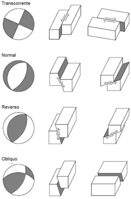
2.2 Mecanismo Focal
PPGG/UFRN Página 23 falha e o respectivo movimento da mesma podem ser visualizados na Figura 2.1.
Figura 2.1 Desenho esquemático ilustrando os componentes (strike, dip e rake) que caracterizam
um plano de falha. (Modificado de Shearer, 2009).
O mecanismo focal, também conhecido como bola de praia (beach ball), é uma forma de representar a falha geológica e o respectivo movimento com os quais um determinado evento sísmico está relacionado e ele é definido pelos seguintes parâmetros: strike (0º≤ ϕ <360º), dip (0º≤δ<90º) e rake
(-180º≤λ<180º). O objetivo de um mecanismo focal é descrever o tipo de falhamentos, bem como estimar a direção dos esforços responsáveis pelo respectivo surgimento do sismo (Lima Neto, 2009).
PPGG/UFRN Página 24
Figura 2.2 Desenho esquemático mostrando a relação entre o plano de falha e o plano auxliar com relação aos quadrantes de empurrão (+) e puxão (-) em torno de um hipocentro (estrela vermelha). Os triângulos pretos representam estações sismográficas, enquanto que os traços pretos (em cima das estações) representam de maneira esquemática os sismogramas da componente vertical de cada estação.
Um dos métodos para determinar o mecanismo focal é fazer uso das polaridades do primeiro movimento das ondas P na componente vertical de cada uma das estações. Assim, se um determinado terremoto for registrado por muitas estações em diferentes direções e distâncias, é possível determinar as direções do plano de falha e do plano auxiliar plotando em uma projeção estereográfica as observações de cada estação (azimute em relação ao epicentro e ângulo de saída). Feito isso, tenta-se encontrar dois plano ortogonais entre si que separem as polaridades positivas e negativas em diferentes quadrantes.
Esse método, por si só, não permite identificar quem é o plano de falha e quem é o plano auxiliar, uma vez que ambos os planos nodais são capazes de reproduzir o mesmo padrão de polaridades. Assim, para identificar o plano de falha, é necessário utilizar informações extras, provenientes de observações geológicas ou mesmo através das réplicas dos sismos. A Figura 2.3 mostra exemplos de mecanismos focais e as respectivas geometrias de falha correspondentes.
PPGG/UFRN Página 25 possuem o mesmo mecanismo focal, de maneira que podem ser representadas de maneira conjunta (Udìas et al., 1985). Contudo, essa técnica deve ser usada com parcimônia, uma vez que nem todos os terremotos irão possuir, de fato, o mesmo mecanismo. Também, se a zona sísmica for muito pequena, as polaridades vão se sobrepor, de maneira que a resolução do mecanismo focal melhorará quase nada.
PPGG/UFRN Página 26
Capítulo 3
–
Metodologia
3.1 Aquisição e análise dos dados
A rede São Rafael, como dito anteriormente, teve suas estações operando por cerca de nove meses e meio. Durante esse período, toda a manutenção e coleta dos dados foi realizada pelos técnicos do LabSis em intervalos regulares de, aproximadamente, quarenta dias. Todos os dados coletados foram armazenados em disco rígido e estão disponíveis no Laboratório Sismológico da UFRN.
Ao longo dos 290 dias de operação, a rede registrou um total de 170 eventos, incluindo tanto os sismos locais, como os regionais e os telessísmicos. Dentre os 170 terremotos registrados, 111 foram locais da barragem do Açu.
No presente estudo, foram utilizados apenas os sismos locais registrados pela rede. Contudo, alguns deles foram utilizados apenas para a contagem de eventos. Isso se deve ao fato de que alguns terremotos que ocorreram foram muito pequenos, microssismos, de modo que não foram registrados, de maneira clara, por pelo menos três estações. Todo o conjunto de dados foi analisado em um PC do LabSis, e se deu no software COMPASS, fornecido pelo fabricante dos registradores (Reftek.).
Primeiramente, a estação BAMZ (Fig. 1.6) foi escolhida com o intuito de fazer uma lista com todos os eventos registrados. Essa estação foi escolhida pelo fato de ela ser a mais próxima da área epicentral.
PPGG/UFRN Página 27 tornaram-se mais fáceis, principalmente para o caso dos eventos menores. Na Figura 3.1 é possível observar um exemplo de um sismograma digital de um dos terremotos registrados.
Figura 3.1 Exemplo digital de terremoto registrado pela estação BAMZ. Também possível observar o instante de chegada das ondas P e S.
PPGG/UFRN Página 28
3.2 Modelo de velocidade e localização epicentral
Após realizar a leitura dos dados, partiu-se para a confecção de um modelo de velocidade, o qual será usado pelo HYPO71 (Lee & Lahr, 1975) na determinação dos parâmetros hipocentrais.
Para calcular o hipocentro dos terremotos, o HYPO71 necessita que seja fornecido, além das coordenadas das estações que compuseram a rede local, um modelo de velocidades que retrate bem a área. Esse modelo é composto pela razão Vp/Vs (razão entre as velocidades das ondas P e S) e a velocidade da onda P para cada camada do modelo de crosta. Neste trabalho, o modelo de crosta utilizado considera que, no local do reservatório, a crosta pode ser representada por um semi-espaço infinito, homogêneo e isotrópico. Esse modelo de crosta foi escolhido pelo fato de o mesmo já ter sido utilizado com sucesso, por outros autores, para a área em questão (Ferreira et al., 1995; Ferreira, 1997; Do Nascimento, 1997; Do Nascimento et al., 2004).
Definido o modelo de crosta, o segundo passo foi obter a razão Vp/Vs. A determinação desse parâmetro se deu por meio do diagrama de Wadati (Fig. 3.2). Esse diagrama consiste de representar graficamente a diferença temporal dos tempos de chegada das ondas P e S (ts – tp) e a diferença entre a primeira chegada da onda P e a hora de origem do evento (tp – to). O gráfico consiste em uma reta que passa pela origem e possui coeficiente angular a=(Vp/Vs) – 1 (Kisslinger & Engdahl, 1973).
PPGG/UFRN Página 29
Figura 3.2 Diagrama Wadati dos 50 eventos selecionados. S-P é a diferença dos tempos de chegada das ondas S e P, enquanto que P-O é a diferença da chegada da onda P e a hora de origem do terremoto. Ambas as diferenças são mostradas em segundos.
Após obter a razão Vp/Vs, o último passo para determinar o modelo de velocidade foi obter o melhor valor de Vp. Esse parâmetro foi obtido por meio de testes realizados no próprio HYPO71. Ao todo, foram realizados 19 testes, nos quais os 50 eventos escolhidos com a ajuda do Wadati (Fig. 3.2) foram localizados utilizando um valor fixado de Vp/Vs=1,67 (obtido no diagrama Wadati) e variando-se Vp. Assim, A velocidade da onda P foi variada de 5,5 a 6,4 Km/s devido ao fato de que trabalho anteriores (Ferreira et al., 1995; do Nascimento et al., 2004) obtiveram, para essa região, Vp=6,00 km/s. Os resultados dos testes podem ser observados na Tabela 3.1.
PPGG/UFRN Página 30 o escolhido como sendo o modelo de velocidades final utilizado na localização dos eventos. A lista dos eventos localizados pelo HYPO71 pode ser visualizada no Apêndice A.
Tabela 3.1 Resultado dos testes para determinação do parâmetro Vp do modelo de velocidades.
3.3 Ajuste do plano e determinação do Mecanismo Focal
Um dos objetivos desse trabalho é a confecção de um Mecanismo Focal a partir dos dados obtidos pela rede São Rafael. O intuito de um mecanismo focal é descrever o falhamento responsável pela atividade sísmica da área, do mesmo modo que estimar os esforços responsáveis por isso. Ele é definido, basicamente, pela direção da falha (Azimute), pelo ângulo do plano de falha (dip) e pela direção do rake.
Teste Vp Vp/Vs RMS (s) ERH (Km) ERZ (Km)
1 5,50 1,67 0,0386 0,1858 0,2633
2 5,55 1,67 0,0350 0,1704 0,2415
3 5,60 1,67 0,0316 0,1567 0,2202
4 5,65 1,67 0,0284 0,1425 0,1998
5 5,70 1,67 0,0253 0,1285 0,1798
6 5,75 1,67 0,0220 0,1142 0,1594
7 5,80 1,67 0,0188 0,0988 0,1379
8 5,85 1,67 0,0158 0,0863 0,1185
9 5,90 1,67 0,0138 0,0767 0,1052 10 5,95 1,67 0,0131 0,0725 0,1027 11 6,00 1,67 0,0136 0,0748 0,1065
12 6,05 1,67 0,0147 0,0800 0,1173
13 6,10 1,67 0,0157 0,0854 0,1323
14 6,15 1,67 0,0165 0,0892 0,1702
15 6,20 1,67 0,0174 0,0933 0,2469
16 6,25 1,67 0,0189 0,1025 0,3063
17 6,30 1,67 0,0207 0,1127 0,2790
18 6,35 1,67 0,0228 0,1248 0,2944
PPGG/UFRN Página 31 Para a determinação do mecanismo focal, o primeiro passo foi ajustar o plano de falha, ou seja, determinar o azimute e o mergulho da falha. Esse ajuste foi feito por meio do método dos quadrados-mínimos. Esse método assume que as coordenadas espaciais dos eventos (latitude, longitude e profundidade) são variáveis independentes, de modo que o se quer minimizar é a distância de cada hipocentro ao plano de falha. Para garantir um bom ajuste do plano, é necessário trabalhar com o melhor conjunto de dados possível, ou seja, devem ser utilizados apenas os sismos que tiveram os menores erros de localização. Com o intuito de garantir que essa necessidade seja atendida, foram utilizados no ajuste do plano apenas os terremotos que satisfizeram os seguintes critérios:
1) Gap < 180, ou seja, os eventos devem estar dentro da rede sismográfica;
2) RMS ≤ 0,013 s;
3) Nº de observações ≥ 10;
4) ERH < 0,1 Km; 5) ERZ < 0,1 Km.
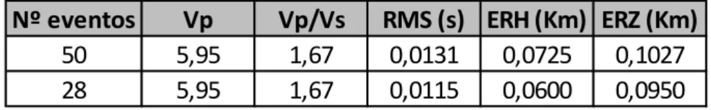
Assim, com base nesses critérios, os 50 eventos localizados pelo HYPO71 foram reduzidos para 28, os quais representam o melhor conjunto de dados possível. A lista dos eventos selecionados pode ser visualizada no Apêndice B. Para comprovar a boa qualidade dos terremotos selecionados, foi confeccionada uma tabela comparativa (Tabela 3.2) entre os 28 e os 50 eventos.
Tabela 3.2 Comparação dos valores de RMZ, ERH e ERZ entre o conjunto total de dados (50 eventos) e 28 sismos selecionados para determinação do mecasnismo focal composto.
O valor do rake, último parâmetro necessário para determinação do mecanismo focal da falha, foi obtido por meio de um ajuste visual. Primeiramente, o valor do azimute e do mergulho obtidos por meio dos quadrados-mínimos foram fixados, enquanto que o valor do rake foi variado
Nº eventos Vp Vp/Vs RMS (s) ERH (Km) ERZ (Km)
50 5,95 1,67 0,0131 0,0725 0,1027
PPGG/UFRN Página 33 Capítulo 4
–
Artigo
Seismicity migration induced by the Açu reservoir, NE Brazil, and implications for fault hydraulic variability
Pedro A. Rodrigues Ferreira1, Joaquim M. Ferreira1, 2, *, Aderson F. do
Nascimento1,2, Francisco H. R. Bezerra1,3, Heleno C. de Lima Neto4, Eduardo
A. S. Menezes2.
1 - Programa de Pós Graduação em Geodinâmica e Geofísica, Universidade Federal do Rio G. do Norte, Campus Universitário, Natal, RN 59078-970, Brazil. 2 - Departamento de Geofísica, Universidade Federal do Rio Grande do Norte, Campus Universitário, Natal, RN 59078-970, Brazil.
3 - Departamento de Geologia, Universidade Federal do Rio Grande do Norte, Campus Universitário, Natal, RN 59078-970, Brazil.
4 - Universidade Potiguar, Escola de Engenharias e Ciências Exatas, Natal, RN 59054-180, Brazil.
PPGG/UFRN Página 34
Abstract
The seismic activity at the Açu reservoir is considered one classical example of
Reservoir-Induced Seismicity and has been extensively investigated in the last
couple of decades. After a long time without activity recorded from there, a new
seismicity was recorded in the area. From the recent digital data acquired, we
were able to determine the hypocentral parameters and focal mechanism of the
new events. Our study reveals the seismic activity in remarkable detail with
vertical and horizontal location errors ≈0.1 km. The earthquakes occurred manly
inside the lake at the depth of 3.5 km in a sub-vertical fault and they were
associated with the reactivation of the basement on a new fault sub-parallel to
the São Rafael Fault. We used the results to seismically derivate hydraulic
diffusivity of the seismogenic fault. Our results showed a fault system being
continuous reactivated mainly due to pore pressure diffusion from surface to
hypocentral depths and they are important for the understanding the interplay
between seismicity, structural geology and hydromechanical properties of faults
and also to constrain the mechanisms that have triggered the seismicity at the
reservoir.
Keywords: reservoir-induced seismicity, triggered seismicity, hydraulic
PPGG/UFRN Página 35
1. Introduction
Human engineering actions can modify the crustal stress in such a way that
earthquakes may be induced or triggered. A few examples of these actions are
the injection of fluids under high pressure into the crust such as hydraulic
fracturing (e.g., Zoback et al., 1997), geothermal power generations and
stimulation (e.g., Majer et al., 2007), secondary oil recovery (e.g., Davies et al.,
2013) and impounding of reservoir behind high dams (Gupta, 1992; Gupta and
Chadha, 1995; Ferreira et al, 1995; Guha, 2000). Around the world, there is a
great number of water reservoirs built with the most different purposes, such as
power generations, irrigation, human consumption, and river flow regulation.
The seismicity related with those dams has an enormous potential to damage
the reservoirs itself and the nearby constructions, what leads to material and in
some cases human loses (Gupta, 1992). Because of this potential threat to
humans and buildings, reservoir induced seismicity (RIS) has received special
attention from researches over the years (Guha, 2000).
The human activity is not the primary cause of the seismicity, but only acts like
a trigger that releases the preexisting stress of tectonic origin (Simpson, 1986).
In other words, the RIS can only occur in areas that are already under
near-critical tectonic stresses. This fact would explain why, even existing a larger
number of water reservoirs on earth, only a small percentage of them have
earthquakes. Many studies were carried out with the objective of understanding
the mechanisms by which earthquakes are induced by reservoirs (e.g., Bell and
Nur, 1978; Simpson et al., 1988; Simpson and Narashimhan, 1990; Knoll, 1990;
PPGG/UFRN Página 36 there are two main effects that influence seismicity. The first one is the rapid or
undrained response, which is attributed to short time scale elastic deformation
of fractures and to existing heterogeneities thereby producing locally high pore
pressure and consequently, locally high stress field (Guha, 2000). The second
one is the delayed or drained response and it has been associated with
diffusion of pore pressure to depths whereby potential faults may be activated
due the lowering of effective stress by the increase of the pore pressure (Guha,
2000).
In addition, faults/fractures hydromechanical characterization is critical when
assessing the delivery of geological carbon storage or radioactive waste
disposal. This characterization can be used to predict the transport of these
substances at depth in a time-scale spanning from hundreds to millions of years
(Olsson & Brown, 1993; Claesson et al., 2007;Zoback and Gorelick, 2012).
In Brazil, there are nineteen seismic areas where induced earthquakes were
reported (Silva, 2011). One of those is the Açu reservoir (Fig. 1). This activity is
considered one classical example of RIS and has been extensively investigated
in the last couple of decades (e.g., Ferreira et al., 1995; do Nascimento, 1997;
do Nascimento et al., 2002, 2004a, 2004b; El Hariri et al., 2010; Telesca et al.,
2012). The Açu reservoir was built in 1983, and seismic monitoring started in
1987. A single-permanent station continuously recorded events in the dam area
from 1987 until 1997 (Fig. 2). Three different campaigns with local seismograph
networks were carried out during this period: the first one from October to
PPGG/UFRN Página 37 the third one between 1994 and 1997 (do Nascimento et al., 2004a). The
activity recorded during these three periods did not occurred in the same area
of the lake, but at four different locations (Fig. 3).
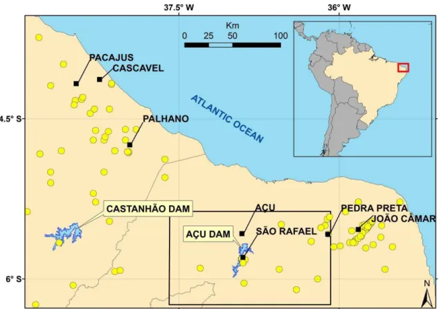
Figure 1 – Location of the Açu and Castanhão dams in northeastern Brazil. The black squares
represent some towns close to epicentral areas. The yellow circles represent earthquakes with
magnitudes higher than 2.0 mb. All the events shown are natural intraplate earthquakes except the
seismicity close to the Açu and Castanhão dams. The black rectangle represents the area shown in
PPGG/UFRN Página 38
Figure 2 – Water level variation (dashed line) and quantity of earthquakes recorded by the station
of BA1 (solid line) from 1987 to 1997 (modified from do Nascimento, 1997).
Figure 3 –Epicentral locations of events recorded during the three campaigns with local networks
PPGG/UFRN Página 39 This seismicity in the Açu reservoir area was first documented by Ferreira et al.
(1995), which used of data provided by the first (1989) and second campaigns
(1990-1991). They observed that the activity increased with a delay of three
months of the water peak of the lake and they conclude that pressure diffusion
through the pores was the dominant mechanism that induced the seismicity.
The spatio-temporal evolution of the earthquakes recorded in the 1994-1997
period form four linear clusters of events, each of which associated with a fault
segment. This result is also consistent with the theory that the mechanism
responsible for triggering the earthquakes is the pore-pressure diffusion (do
Nascimento et al., 2004a).
The continuous seismic monitoring was interrupted and no more events were
recorded in the Açu reservoir area by regional seismographic stations after
1997. After a long time without seismic activity, an earthquake with regional
magnitude (Assumpção, 1983) mR=1.3 was recorded in June 2012 by a sensor
located 116 km from the Açu reservoir. The preliminary analysis suggested that
this event was related with a new epicentral area, which was located in a
different fault. This activity encouraged the installation of a new local
seismographic network (São Rafael seismograph network) to record the new
seismic activity (Fig. 4).
Although several studies have been carried out in the Açu reservoir area, the
new data can shed light on some important RIS scientific gaps. First, it is usual
PPGG/UFRN Página 40 earthquakes (Carena et al., 2002; Geiser and Seeber, 2008; Julian et al., 2010). However, seismogenic faults in the Açu reservoir area have a more complex
expression over space and time (Pytharouli et al., 2011) than can only be
revealed by precise hypocentral location and proper seismic monitoring.
Second, it is still not know if reservoir seismicity in the region can occur
repeatedly over a long time span, reactivating or creating different fault
segments. Third, it is still a matter of debate which mechanism have generated
RIS in the region: either local stress field change or diffusion of pore pressure.
Figure 4 – Map of the São Rafael seismograph network, which was composed of eight stations and
PPGG/UFRN Página 41 The objective of this work is (1) to determine the hypocentral parameters and
focal mechanism of the new events in the Açu reservoir area to verify if they are
related with a previous or new epicentral area and (2) to assess the
mechanisms that have triggered the seismicity. Therefore, we describe the new
seismic activity and compare it with the three previous periods of induced
seismicity. We concluded that this new seismic activity vindicates the previous
hypothesis of pore-pressure diffusion at a different fault segment. This study
has implications for understanding the interplay between seismicity, structural
geology and hydromechanical properties of faults. The values of the seismically
derived hydraulic properties in our studies are compatible with previous
estimates and reveal a great spatial and temporal variability of these properties.
This work sheds further light on how RIS can be used to characterized fluid flow
in rocks.
2. Seismological and tectonic settings
Northeastern Brazil is characterized by intense natural intraplate seismicity (Fig.
1). The region has been affected by earthquake sequences that last up to ten
years with magnitudes up to 5.2 mb. The depth of the natural seismicity ranges
from 1 to 12 km and it is mainly characterized by strike-slip earthquakes
(Ferreira et al., 1995, 1998, 2008; Do Nascimento et al., 2002, 2004a).
The Açu reservoir is located in the state of Rio Grande do Norte, northeastern
PPGG/UFRN Página 42 reservoir in the region, second only to the Castanhão dam, located in state of
Ceará (Fig. 1). Both of them exhibited RIS (Ferreira et al., 1995, 2008).
Geologically, the study area is located in the Precambrian crystalline basement
known as the Borborema Province. The region was affected by the Brasiliano
orogenic cycle from 740-540 Ma (Almeida et al., 2000) and the breakup
between Africa and South America in the Cretaceous (De Castro et al., 2012;
Bezerra et al., 2014).The study area is also close to the Potiguar Basin, which
was formed during in the Cretaceous (Matos, 1992). The lithology that
surrounds the dam is mostly composed of gneisses and granitic rocks, which
are cut across by Jurassic-Cretaceous E-W-oriented basalt dikes (Fig. 5).
Figure 5 – Simplified geological map of the Borborema Province around the Açu dam (CPRM,
2006). The reservoir is located on the south of the Potiguar basin and is surrounded by
metamorphic and igneous rocks. The map also shows the NE-SW trending faults and E-W dikes
PPGG/UFRN Página 43 This crystalline basement has high rigidity, simple seismic velocity structure and
low attenuation. Those characteristic lead to simple and impulsive P and S
wave arrivals and high signal-to-noise ratios (Takeya et al. 1989; Ferreira et al., 1995, 1998; do Nascimento et al., 2004a; Lima Neto, 2013; Telesca et al., 2012; Oliveira et al., 2015).
The dam’s surrounding area contains a series of NE–SW-striking faults and
fractures, which reactivated the ductile Precambrian shear zones (Bezerra and
Vita-Finzi, 2000; Do Nascimento et al., 2004a; Bezerra et al., 2014). Earthquake
alignments and focal planes associated with the Açu RIS exhibits a similar
trend, which suggests fault reactivation. At the scale of hundreds of meters,
however, faults cut across the main ductile mylonitic fabric indicating that the
reactivation process is scale-dependent (Kirkpatrick et al., 2013). The main fault
segment in the study area is the São Rafael Fault (SRF), which is ~ 18 km long
and is composed of cataclastic rocks with intrusions of quartz veins. The
epicenters of the 94-97 activity matches with the SRF, which indicates that this
seismicity was generated by the reactivation of this fault (Amaral, 2000). In this
case, it indicates that the fluid triggered the fault reactivation.
3. Methods
3.1. Data acquisition and processing
The seismic activity was recorded by the São Rafael seismograph network,
which was composed of eight stations and acquired data from July 2012 until
PPGG/UFRN Página 44 seismometer L4-3D model and a Reftek130 recorder, using the sample rate of
500 samples per second. The record reading (arrival time and polarities of P
and S) and processing was carried out with the COMPASS software provided
by Reftek. An example of the earthquakes recordings can be seeing in Figure 6.
The total number of events was used to analyze the relation between the
seismicity and water level and the best recorded events were used to determine
the velocity model and the focal mechanism.
Figure 6 – Example of one digital seismogram of an earthquake recorded by the BAMZ station.
3.2. Hypocentral parameters
The hypocentral parameters were determined with HYPO71 (Lee and Lahr,
1975), which needed to be filed with a velocity model of the study area. We
assumed the crust to be a homogenous and isotropic half-space. We choose
this model because it was successfully used in previous studies (e.g., Ferreira
PPGG/UFRN Página 45 The next step was to determine the VP/VS ratio. This value was obtained using
the Wadati diagram (Fig. 7). In addition, this diagram was important because it
allowed us to verify the consistency of the readings. We used 50 from 111
events recorded by the local network in the Wadati diagram, which corresponds
to 285 readings. We found a VP/VS = 1.67 (Fig. 7). We carried out 19
simulations using HYPO71 to find the best VP value, in which we varied the
values of VP from 5.50 to 6.40 km/s with the VP/VS ratio fixed at 1.67. At the end
of these searches, VP = 5.95 km/s was the value that presented the lowest
mean errors in residual mean squared (s) and in horizontal (km) and vertical
(km) locations.
Figure 7 – Wadati diagram for the Açu dam determined with 50 events. The best fit (solid red line)
indicates VP/VS = 1.67 (±0.003). S-P is the difference between the arrival times of the S and P waves,
while P-O is the difference between the P arrival time and the origin time of the earthquake. Both
PPGG/UFRN Página 46
3.3. Determination of the focal mechanism
To obtain the fault plane, we used the least-square method. This method
assumes that latitude, longitude and depth are independent variables, in a way
that allow us to minimize the distance of each hypocenter to the fault plane (do
Nascimento, 1997). To adjust this plane, it is necessary to use events with the
lowest location errors. To ensure this condition, we selected those events from
the 50 events located by the HYPO71 with the following characteristics: at least
10 P and S readings (NO ≥ 10), arrival-time residual (rms) ≤ 0.013 s, vertical
error (erz) < 0.1 km, and horizontal error (erh) < 0.1 km. We obtained 28
earthquakes that obeyed these criteria. With this method, we calculated fault
strike and dip. The values obtained by the least-square method were fixed and,
together with the plot of the P-wave polarities, we obtained the rake through a
visual inspection.
4. Results
4.1. Epicentral and Hypocentral location
The results provided by HYPO71 (Fig. 8) were of excellent quality, which is
attested by the average errors of the 50 events (rms = 0.013 s, erh = 0.072 km,
and erz = 0.103 km). The epicentral map indicates that the recent seismic
activity was mainly concentrated inside the lake 7 km to the southwest of the
town of São Rafael. Therefore, these new data indicate that the Açu RIS
migrated again to a new epicentral area. There were six additional events
located in different locations away from the cluster. The first three occurred to
the northeast of the BAPO station, whereas the last three occurred to the north
PPGG/UFRN Página 47 The main seismic activity occurred in a seismogenic zone ~ 1 km long with the
shallowest and deepest earthquakes occurring at 3.1 and 4.3 km, respectively.
The greatest number of events was located around 3.5 km depth (Fig. 9). The
depth variation of the earthquakes was almost constant. This average depth of
the recent events is similar to the 1989 activity, which also happened below the
lake and was more than 3 km deep.
Figure 8 – Map of epicentral location of 50 selected events calculated with HYPO71. The red circle
indicates the main seismogenic zone of the recent activity. This main cluster occurred inside the
PPGG/UFRN Página 48
Figure 9 – Depth variation of the activity in the main cluster. The 44 events sampled are presented
in their respective occurrence order. It is possible to notice that the most of the events occurred
around 3.5 km depth.
4.2. Focal mechanism
The 28 events selected to determine the focal mechanism by the least-square
method provided the adjusted plane. Figure 10 provides the hypocentral
distribution and the fault direction and dip. It shows the depth distribution of the
28 events, which are exhibited in two planes: one parallel to the fault strike (Fig.
10b) and orthogonal to the fault strike (Fig. 10c). These figures depict the
PPGG/UFRN Página 49
Figure 10 – (a) Map of the 28 events selected to determine the focal mechanism. The blue arrows
indicate the directions of the (b) and (c) projections. The blue triangle indicates the closest station
(BAMZ) of the selected events; (b Along-strike vertical projection of seismicity with NW-SE
direction (149º azimuth); (c) projection orthogonal to fault strike with SW-NE direction (59º
azimuth). The circles represent the events with depth between 3.23 and 3.46 km, whereas the
PPGG/UFRN Página 50 We obtained a composite focal mechanism for the new seismic area
underneath the Açu reservoir. The rake was determined through visual fit,
making use of the stations with alternating polarities, which indicates proximity
to one of the nodal planes. The focal mechanism indicates a fault with the
following parameters: strike = 59º, dip = 84 º and rake = -170 (Fig. 11). The
mechanism indicates that the fault is approximately vertical and strikes NE–SW,
with a strike-slip movement.
Figure 11 – Composite focal mechanism for the recent activity in the Açu dam. Crosses and circles
represent the first movements of compression and dilation, respectively. P and T are the axes of
PPGG/UFRN Página 51 Figure 12 exhibits the 28 events selected to determine the focal mechanism and
the surface projection of the seismogenic fault. The results of our study are
consistent with the NE–SW-striking faults previously determined in the Açu
reservoir area by Ferreira et al. (1995) and do Nascimento et al. (2004b). From
SLAR images obetined before the Açu reservoir impoundment, do Nascimento
et al. (2004a) identified lineaments associated with ductile Precambrian fabric
(foliations and shear zones). This ductile fabric mainly strikes NE-SW (Fig. 12).
Figure 12 – Plane projection of the fault determined using the least-square method and the main
PPGG/UFRN Página 52 The focal mechanism of the present study is very similar to those determined in
the previous studies. Figure 13 shows the distribution of all the earthquakes
located in the area, including those presented for the first time in our study, as
well the related four focal mechanisms. The comparisons of the strike and dip of
the nodal planes of all focal mechanisms (Fig. 14) indicates that they are similar
and consistent with the regional stress field (Ferreira et al., 1998).
The Figure 15 shows the spatial evolution of the seismic activity of the main
epicentral area. The distance showed in Figure 15 was measured from the
BAPO station (Fig. 4) because it was located along the fault strike. It is possible
to see that in the plan view, the fault movement occurred in two main fault
segments, both of them with NE-SW strike.
Figure 13 – Epicenters of the three previous periods of seismic activity and events reported in the
PPGG/UFRN Página 53
Figure 14 – Focal mechanisms of the four periods of RIS in the Açu dam area. It is possible to
notice their direction and dip similarities and the overall consistency with the regional stress
PPGG/UFRN Página 54
Figure 15 – Spatial evolution of the seismic activity along the fault strike. The reference point of
axis Y (vertical axis) is the BAPO station coordinates (36.8976 W, 5.8307 S). This coordinate was
chosen because it is located along the fault strike. It is possible to see that the rupture occurred in
two main fault segments (red solid lines), both of them along the NE-SW direction. The first from
4550 to 4650 m far from the central point and the second from 4300 to 4400 m.
5. Discussion
Figure 16 exhibits the monthly variations of the water level of the Açu reservoir
from January 2009 until June 2013 and the amount of earthquakes recorded by
the São Rafael network during the time it was carried on. The great number of
events was recorded in July and August 2012. However, but the increasing in
the seismicity started in the second half of June 2012, with the earthquakes
PPGG/UFRN Página 55 network. This late deployment resulted in a delay time between 11 and 12
months after the previous water peak in July of 2011. This delay time (time
difference between the water level peak and the increase of seismicity) is much
longer than those previously recorded. Ferreira et al. (1995) pointed a delay of
only three months in the 1989 activity. Do Nascimento el al. (2004a) were able
to identify three activity clusters with three different delay times of 4.5, 6 and 7
months at three different depths (2, 2.8 and 4.3 km, respectively) for the 94-97
activity. They observed that the delay increased with the cluster hypocenter
depth. These different delay times could had been associated with different
faults with different hydraulic properties, as suggested by do Nascimento et al.
(2004a).
Figure 16 – Water level variation from January 2009 until June 2013 and the number of earthquakes
recorded by the São Rafael seismograph network. The peak of seismicity occurred 12 months after
the last peak of the water level. We used this delay time to calculate the hydraulic diffusivity.
Northeastern Brazil is a region with significant natural seismicity, and nearby
PPGG/UFRN Página 56 shown in Figure 1 (e.g., Assumpção et al., 1985; Ferreira, 1997; Ferreira et al.,
1998; Lima Neto et al., 2013; Oliveira et al., 2015), what always leaves open the
possibility of the seismicity being natural. However, the 2012-2013 seismicity
exhibits characteristics similar to the previous RIS periods. First, it presents a
similar strike-slip focal mechanism, with a NE-SW-striking fault plane and a
right-lateral sense of movement. Second, it occurred underneath the Açu
reservoir at depths similar to those of the previous RIS periods. These features
indicate that the 2012-2013 seismicity was a new RIS case induced by the Açu
reservoir.
Studying the 1994-1997 data, Pytharouli et al. (2011) were able to conclude that
the seismic activity that was associated with the São Rafael fault (SRF) did not
occur on a single surface defined by the best-fitting plane to the events location.
Instead, this seismicity occurred on multiple planes. The low angle between our
adjusted plane and the SRF is caused by the fact that not all events have
occurred in the central fault, some of them occurred on subsidiary faults. This
hypothesis agrees with the conceptual model of a fault developed in a region
with a pre-existing shear zone defined by mylonitic foliation presented by
Kirkpatrick et al. (2013).
A way to obtain information to infer if the seismicity is related with the water
reservoir is making use of concept of the seismic hydraulic diffusivity (αs)
(Talwani et al., 2007). They found that the typical range of αs varies between 0.1
and 10 m²/s. They defined αs=L²/4Δt, where L is the characteristic distance