Contents lists available atScienceDirect
Physics Letters B
www.elsevier.com/locate/physletb
Angular analysis and branching fraction measurement of the decay
B
0
→
K
∗
0
μ
+
μ
−
✩
.
CMS Collaboration
⋆
CERN, Switzerland
a r t i c l e
i n f o
a b s t r a c t
Article history:
Received 15 August 2013
Received in revised form 1 October 2013 Accepted 7 October 2013
Available online 15 October 2013 Editor: M. Doser
Keywords: CMS Physics
The angular distributions and the differential branching fraction of the decay B0
→K∗(892)0
μ
+μ
−are studied using a data sample corresponding to an integrated luminosity of 5.2 fb−1 collected with
the CMS detector at the LHC in pp collisions at√s=7 TeV. From more than 400 signal decays, the forward–backward asymmetry of the muons, the K∗(892)0 longitudinal polarization fraction, and the differential branching fraction are determined as a function of the square of the dimuon invariant mass. The measurements are in good agreement with standard model predictions.
2013 CERN. Published by Elsevier B.V. All rights reserved.
1. Introduction
It is possible for new phenomena (NP) beyond the standard model (SM) of particle physics to be observed either directly or indirectly, i.e., through their influence on other physics processes. Indirect searches for NP generally proceed by comparing experi-mental results with theoretical predictions in the production or decay of known particles. The study of flavor-changing neutral-current decays of b hadrons such as B0
→
K∗0μ
+μ
−(K∗0indicates the K∗(
892)
0 and charge conjugate states are implied in what fol-lows, unless explicitly stated otherwise) is particularly fertile for new phenomena searches, given the modest theoretical uncertain-ties in the predictions and the low rate as the decay is forbidden at tree level in the SM. On the theoretical side, great progress has been made since the first calculations of the branching fraction [1–4], the forward–backward asymmetry of the muons, AFB [5], and the longitudinal polarization fraction of the K∗0, FL [6–11]. Robust calculations of these variables [12–19] are now available for much of the phase space of this decay, and it is clear that new physics could give rise to readily observable effects [8,16,20–34]. Finally, this decay mode is relatively easy to select and reconstruct at hadron colliders.The quantities AFB and FL can be measured as a function of the dimuon invariant mass squared
(
q2)
and compared to SM predictions[14]. Deviations from the SM predictions can indicate✩ © CERN for the benefit of the CMS Collaboration.
⋆ E-mail address:[email protected].
new physics. For example, in the minimal supersymmetric stan-dard model (MSSM) modified with minimal flavor violation, called flavor blind MSSM (FBMSSM), effects can arise through NP con-tributions to the Wilson coefficient C7 [16]. Another NP example is the MSSM with generic flavor-violating and CP-violating soft SUSY-breaking terms (GMSSM), in which the Wilson coefficients C7, C′
7, and C10 can receive contributions [16]. As shown there, these NP contributions can dramatically affect the AFB distribu-tion (note that the variable Ss6 defined in Ref. [16] is related to AFB measured in this Letter by Ss6
= −
43AFB), indicating that pre-cision measurements of AFB can be used to identify or constrain new physics.While previous measurements by BaBar, Belle, CDF, and LHCb are consistent with the SM [35–38], these measurements are still statistically limited, and more precise measurements offer the pos-sibility to uncover physics beyond the SM.
In this Letter, we present measurements of AFB,FL, and the dif-ferential branching fraction d
B
/
dq2 from B0→
K∗0μ
+μ
− decays, using data collected from pp collisions at the Large Hadron Collider (LHC) with the Compact Muon Solenoid (CMS) experiment in 2011 at a center-of-mass energy of 7 TeV. The analyzed data correspond to an integrated luminosity of 5.
2±
0.
1 fb−1[39]. The K∗0is recon-structed through its decay to K+π
−and the B0is reconstructed by fitting the two identified muon tracks and the two hadron tracks to a common vertex. The values of AFB and FL are measured by fitting the distribution of events as a function of two angular vari-ables: the angle between the positively charged muon and the B0 in the dimuon rest frame, and the angle between the kaon and theB0 in the K∗0 rest frame. All measurements are performed in q2 bins from 1 to 19 GeV2. Theq2 bins 8
.
68<
q2<
10.
09 GeV2 and 12.
90<
q2<
14.
18 GeV2, corresponding to the B0→
K∗0J/ψ
andB0
→
K∗0ψ
′ decays (ψ
′ indicates theψ (
2S)
in what follows), re-spectively, are both used to validate the analysis, and the former is used to normalize the branching fraction measurement.2. CMS detector
A detailed description of the CMS detector can be found else-where [40]. The main detector components used in this analysis are the silicon tracker and the muon detection systems. The sili-con tracker measures charged particles within the pseudorapidity range
|
η
|
<
2.
4, whereη
= −
ln[
tan(θ/
2)
]
andθ
is the polar an-gle of the track relative to the beam direction. It consists of 1440 silicon pixel and 15 148 silicon strip detector modules and is lo-cated in the 3.8 T field of the superconducting solenoid. The re-constructed tracks have a transverse impact parameter resolution ranging from≈
100 µm to≈
20 µm as the transverse momentum of the track (pT) increases from 1 GeV to 10 GeV. In the same pT regime, the momentum resolution is better than 1% in the central region, increasing to 2% atη
≈
2, while the track reconstruction ef-ficiency is nearly 100% for muons with|
η
|
<
2.
4 and varies from≈
95% atη
=
0 to≈
85% at|
η
| =
2.
4 for hadrons. Muons are mea-sured in the pseudorapidity range|
η
|
<
2.
4, with detection planes made using three technologies: drift tubes, cathode strip chambers, and resistive-plate chambers, all of which are sandwiched between the solenoid flux return steel plates. Events are selected with a two-level trigger system. The first level is composed of custom hardware processors and uses information from the calorimeters and muon systems to select the most interesting events. The high-level trigger processor farm further decreases the event rate from nearly 100 kHz to around 350 Hz before data storage.3. Reconstruction, event selection, and efficiency
The signal (B0
→
K∗0μ
+μ
−) and normalization/control samples (B0→
K∗0J/ψ
and B0→
K∗0ψ
′) were recorded with the same trig-ger, requiring two identified muons of opposite charge to form a vertex that is displaced from the pp collision region (beamspot). The beamspot position and size were continuously measured from Gaussian fits to reconstructed vertices as part of the online data quality monitoring. Five dimuon trigger configurations were used during 2011 data taking with increasingly stringent requirements to maintain an acceptable trigger rate as the instantaneous lu-minosity increased. For all triggers, the separation between the beamspot and the dimuon vertex in the transverse plane was re-quired to be larger than three times the sum in quadrature of the distance uncertainty and the beamspot size. In addition, the cosine of the angle between the dimuon momentum vector and the vector from the beamspot to the dimuon vertex in the trans-verse plane was required to be greater than 0.9. More than 95% of the data were collected with triggers that required single-muon pseudorapidity of|
η
(
μ
)
|
<
2.
2 for both muons, dimuon transverse momentum ofpT(
μμ
) >
6.
9 GeV, single-muon transverse momen-tum for both muons of pT(
μ
) >
3.
0,
4.
0,
4.
5,
5.
0 GeV (depending on the trigger), and the corresponding vertex fit probability ofχ
prob2>
5%,
15%,
15%,
15%. The remaining data were obtained from a trigger with requirements of|
η
(
μ
)
|
<
2.
5,χ
prob2>
0.
16%, and pT(
μμ
) >
6.
5 GeV. The events used in this analysis passed at least one of the five triggers.The decay modes used in this analysis require two recon-structed muons and two charged hadrons, obtained from offline reconstruction. The reconstructed muons are required to match the muons that triggered the event readout and to pass several muon
identification requirements, namely a track matched with at least one muon segment, a track fit
χ
2per degree of freedom less than 1.8, at least 11 hits in the tracker with at least 2 from the pixel de-tector, and a transverse (longitudinal) impact parameter less than 3 cm (30 cm). The reconstructed dimuon system is further required to satisfy the same requirements as were used in the trigger. In events where multiple trigger configurations are satisfied, the re-quirements associated with the loosest trigger are used.While the muon requirements are based on the trigger and a CMS standard selection, most of the remaining selection criteria are optimized by maximizing S
/
√
S+
B, whereS is the expected signal yield from Monte Carlo (MC) simulations and B is the back-ground estimated from invariant-mass sidebands in data, defined as>
3σ
m(B0) and<
5.
5σ
m(B0)from the B0 mass[41], whereσ
m(B0)is the average B0 mass resolution of 44 MeV. The optimization is performed on one trigger sample, corresponding to an inte-grated luminosity of 2
.
7 fb−1, requiring 1.
0<
q2<
7.
3 GeV2 or 16<
q2<
19 GeV2 to avoid J/ψ
andψ
′contributions. The hadron tracks are required to fail the muon identification criteria, and have pT(
h) >
0.
75 GeV and an extrapolated distance of closest ap-proach to the beamspot in the transverse plane greater than 1.3 times the sum in quadrature of the distance uncertainty and the beamspot transverse size. The two hadrons must have an invariant mass within 80 MeV of the nominal K∗0 mass for either the K+π
− or K−π
+ hypothesis. To remove contamination fromφ
decays, the hadron-pair invariant mass must be greater than 1.035 GeV when the charged K mass is assigned to both hadron tracks. The B0 candidates are obtained by fitting the four charged tracks to a common vertex and applying a vertex constraint to improve the resolution of the track parameters. The B0 candidates must have pT(
B0) >
8 GeV,|
η
(
B0)
|
<
2.
2, vertex fit probabilityχ
prob2>
9%, vertex transverse separation from the beamspot greater than 12 times the sum in quadrature of the separation uncertainty and the beamspot transverse size, and cosα
xy>
0.
9994, whereα
xy is the angle, in the transverse plane, between the B0 momentum vec-tor and the line-of-flight between the beamspot and the B0 vertex. The invariant mass of the four-track vertex must also be within 280 MeV of the world-average B0mass for either the K−π
+μ
+μ
− or K+π
−μ
+μ
− hypothesis. This selection results in an average of 1.06 candidates per event in which at least one candidate is found. A single candidate is chosen from each event based on the best B0 vertex fitχ
2.The four-track vertex candidate is identified as a B0
(
B0)
if the K+π
−(
K−π
+)
invariant mass is closest to the nominal K∗0 mass. In cases where both Kπ
combinations are within 50 MeV of the nominal K∗0 mass, the event is rejected since no clear identifica-tion is possible owing to the 50 MeV natural width of the K∗0. The fraction of candidates assigned the incorrect state is estimated from simulations to be 8%.From the retained events, the dimuon invariant mass q and its corresponding calculated uncertainty
σ
q are used to distin-guish between the signal and normalization/control samples. The B0→
K∗0J/ψ
and B0→
K∗0ψ
′samples are defined asmJ/ψ−
5σ
q<
q<
mJ/ψ+
3σ
q and|
q−
mψ′|
<
3σ
q, respectively, wheremJ/ψ andmψ′ are the world-average mass values. The asymmetric selec-tion of the J
/ψ
sample is due to the radiative tail in the dimuon spectrum, while the smaller signal in theψ
′mode made an asym-metric selection unnecessary. The signal sample is the complement of the J/ψ
andψ
′samples.The global efficiency,
ǫ
, is the product of the acceptance and the trigger, reconstruction, and selection efficiencies, all of which are obtained from MC simulations. The pp collisions are simulated usingpythia[42]version 6.424, the unstable particles are decayedby evtgen [43] version 9.1 (using the default matrix element for
Fig. 1.Sketch showing the definition of the angular observables for the decay B0→
K∗0(K+π−)μ+μ−.
of the detector with Geant4 [44]. The reconstruction and event
selection for the generated samples proceed as for the data events. Three simulation samples were created in which the B0was forced to decay to B0
→
K∗0(
K+π
−)
μ
+μ
−, B0→
K∗0(
K+π
−)
J/ψ (
μ
+μ
−)
,or B0
→
K∗0(
K+π
−)ψ
′(
μ
+μ
−)
. The acceptance is calculated as the fraction of events passing the single-muon cuts ofpT(
μ
) >
2.
8 GeV and|
η
(
μ
)
|
<
2.
3 relative to all events with a B0in the event with pT(
B0) >
8 GeV and|
η
(
B0)
|
<
2.
2. The acceptance is obtained from the generated events before the particle tracing withGeant4. Toobtain the reconstruction and selection efficiency, the MC simu-lation events are divided into five samples, appropriately sized to match the amount of data taken with each of the five triggers. In each of the five samples, the appropriate trigger and match-ing offline event selection is applied. Furthermore, each of the five samples is reweighted to obtain the correct distribution of pileup events (additional pp collisions in the same bunch crossing as the collision that produced the B0 candidate), corresponding to the data period during which the trigger was active. The reconstruction and selection efficiency is the ratio of the number events that pass all the selections and have a reconstructed B0compatible with the generated B0 in the event relative to the number of events that pass the acceptance criteria. The compatibility of generated and reconstructed particles is enforced by requiring the reconstructed K+,
π
−,μ
+, andμ
− to have(
η
)
2+
(
ϕ
)
2<
0.
3 for hadrons and 0.004 for muons, whereη
andϕ
are the differences inη
andϕ
between the reconstructed and generated particles, andϕ
is the azimuthal angle in the plane perpendicular to the beam di-rection. The efficiency and purity of this compatibility requirement are greater than 99%.4. Analysis method
The analysis measuresAFB, FL, and d
B
/
dq2 of the decay B0→
K∗0μ
+μ
− as a function of q2. Fig. 1shows the relevant angular observables needed to define the decay:θ
K is the angle between the kaon momentum and the direction opposite to the B0(
B0)
in the K∗0(
K∗0)
rest frame,θ
l is the angle between the positive (negative) muon momentum and the direction opposite to the B0
(
B0)
in the dimuon rest frame, andφ
is the angle between the plane containing the two muons and the plane containing the kaon and pion. Since the extracted angular parameters AFB and FL and the acceptance times efficiency do not depend onφ
,φ
is inte-grated out. Although the K+π
−invariant mass must be consistent with a K∗0, there can be contributions from a spinless (S-wave) K+π
− combination[45–47]. This is parametrized with two terms related to the S-wave fraction,FS, and the interference amplitude between the S-wave and P-wave decays, AS. Including this com-ponent, the angular distribution of B0→
K∗0μ
+μ
− can be written as[47]:1
Γ
d3
Γ
d cos
θ
Kd cosθ
ldq2=
169 2 3FS+
4
3AScos
θ
K1
−
cos2θ
l+
(
1−
FS)
2FLcos2
θ
K1−
cos2θ
l+
12(
1−
FL)
1−
cos2θ
K1+
cos2θ
l+
43AFB1−
cos2θ
Kcosθ
l.
(1)The main results of the analysis are extracted from unbinned extended maximum-likelihood fits in bins ofq2to three variables: the K+
π
−μ
+μ
− invariant mass and the two angular variablesθ
K andθ
l. For eachq2 bin, the probability density function (PDF) has the following expression:(
m,
cosθ
K,
cosθ
l)
=
YS·
S(
m)
·
S(
cosθ
K,
cosθ
l)
·
ǫ
(
cosθ
K,
cosθ
l)
+
YBc·
Bc(
m)
·
Bc(
cosθ
K)
·
Bc(
cosθ
l)
+
YBp·
Bp(
m)
·
Bp(
cosθ
K)
·
Bp(
cosθ
l).
(2) The signal yield is given by the free parameterYS. The signal shape is described by the product of a function S(
m)
of the invariant mass variable, the theoretical signal shape as a function of two angular variables, S(
cosθ
K,
cosθ
l)
, and the efficiency as a function of the same two variables,ǫ
(
cosθ
K,
cosθ
l)
. The signal mass shape S(
m)
is the sum of two Gaussian functions with a common mean. While the mean is free to float, the two resolution parameters and the relative fraction are fixed to the result from a fit to the sim-ulated events. The signal angular function S(
cosθ
K,
cosθ
l)
is given by Eq. (1). The efficiency functionǫ
(
cosθ
K,
cosθ
l)
, which also ac-counts for mistagging of a B0 as a B0 (and vice versa), is obtained by fitting the two-dimensional efficiency histograms (6 cosθ
K bins and 5 cosθ
l bins) to polynomials in cosθ
K and cosθ
l. The cosθ
K polynomial is degree 3, while the cosθ
l polynomial is degree 6, with the 1st and 5th orders removed, as these were the simplest polynomials that adequately described the efficiency in all bins. For some q2 bins, simpler polynomials are used as they are sufficient to describe the data. There are two contributions to the back-ground, with yields given byYBpfor the “peaking” background and YBc for the “combinatorial” background. The peaking background is due to the remaining B0→
K∗0J/ψ
and B0→
K∗0ψ
′ decays, not removed by the dimuon mass or q2 requirements. For these events, the dimuon mass is reconstructed far from the true J/ψ
or
ψ
′mass, which results in a reconstructed B0mass similarly dis-placed from the true B0mass. The shapes of this background in the mass, Bp(
m)
, and angular variables, Bp(
cosθ
K)
andBp(
cosθ
l)
, are obtained from simulation of B0→
K∗0J/ψ
and B0→
K∗0ψ
′events, fit to the sum of two Gaussian functions in mass and polynomi-als in cosθ
Kand cosθ
l. The background yield is also obtained from simulation, properly normalized by comparing the reconstructed B0→
K∗0J/ψ
and B0→
K∗0ψ
′ yields in data and MC simulation. The remaining background, combinatorial in nature, is described by a single exponential in mass, Bc(
m)
, and a polynomial in each angular variable,Bc(
cosθ
K)
andBc(
cosθ
l)
, varying between degree 0 and 4, as needed to describe the data.The results of the fit in eachq2 bin (including the J
/ψ
andψ
′parameter is not constrained. The first fit to the data is to the control samples: B0
→
K∗0J/ψ
and B0→
K∗0ψ
′. The values for F S and AS from the B0→
K∗0J/ψ
fit are used in the signalq2 bins, with Gaussian constraints defined by the uncertainties from the fit. The longitudinal polarization fractionFL and the scalar fraction FS are constrained to lie in the physical region of 0 to 1. In ad-dition, penalty terms are added to ensure that|
AFB|
<
34(
1−
FL)
and
|
AS|
<
12[
FS+
3FL(
1−
FS)
]
, which are necessary to avoid a negative decay rate.The differential branching fraction, d
B
/
dq2, is measured rela-tive to the normalization channel B0→
K∗0J/ψ
usingd
B
(
B0→
K∗0μ
+μ
−)
dq2
=
YS
YN
ǫ
Nǫ
Sd
B
(
B0→
K∗0J/ψ )
dq2
,
(3)where YS and YN are the yields of the signal and normalization channels, respectively,
ǫ
S andǫ
N are the efficiencies of the signal and normalization channels, respectively, andB
(
B0→
K∗0J/ψ )
is the world-average branching fraction for the normalization chan-nel [41]. The yields are obtained with fits to the invariant-mass distributions and the efficiencies are obtained by integrating over the angular variables using the values obtained from the previously described fits.Three methods are used to validate the fit formalism and re-sults. First, 1000 pseudo-experiment samples are generated in each q2 bin using the PDF in Eq.(2). The log-likelihood values obtained from the fits to the data are consistent with the distributions from the pseudo-experiments, indicating an acceptable goodness of fit. The pull distributions obtained from the pseudo-experiments in-dicate the uncertainties returned by the fit are generally overesti-mated by 0–10%. No attempt is made to correct the experimental uncertainties for this effect. Second, a fit is performed to a sample of MC simulation events that approximated the data sample in size and composition. The MC simulation sample contains a data-like mixture of four types of events. Three types of events are gen-erated and simulated events from B0
→
K∗0μ
+μ
−, B0→
K∗0J/ψ
,and B0
→
K∗0ψ
′ decays. The last event type is the combinatorial background, which is generated based on the PDF in Eq.(2). Third, the fit is performed on the normalization/control samples and the results compared to the known values. Biases observed from these three checks are treated as systematic uncertainties, as described in Section5.5. Systematic uncertainties
A variety of systematic effects are investigated and the impacts on the measurements ofFL, AFB, and d
B
/
dq2 are evaluated.The finite sizes of the MC simulation samples used to measure the efficiency introduce a systematic uncertainty of a statistical nature. Alternative efficiency functions are created by randomly varying the parameters of the efficiency polynomials within the fitted uncertainties for the MC samples. The alternative efficiency functions are applied to the data and the root-mean-squares of the returned values taken as the systematic uncertainty.
The fit algorithm is validated by performing 1000 pseudo-experiments, generated and fit with the PDF of Eq.(2). The aver-age deviation of the 1000 pseudo-experiments from the expected mean is taken as the systematic uncertainty associated with pos-sible bias from the fit algorithm. This bias is less than half of the statistical uncertainty for all measurements. Discrepancies between the functions used in the PDF and the true distribution can also give rise to biases. To evaluate this effect, a MC simulation sam-ple similar in size and composition to the analyzed data set is fit using the PDF of Eq. (2). The differences between the fitted val-ues and the true valval-ues are taken as the systematic uncertainties associated with the fit ingredients.
Mistagging a B0 as a B0(and vice versa) worsens the measured B0 mass resolution. A comparison of resolutions for data and MC simulations (varying the mistag rates in the simulation) indicates the mistag rate may be as high as 12%, compared to the value of 8% determined from simulation. The systematic uncertainty in the mistag rate is obtained from the difference in the final measure-ments when these two values are used.
The systematic uncertainty related to the contribution from the K
π
S-wave (and interference with the P-wave) is evaluated by tak-ing the difference between the default results, obtained by fitttak-ing with a function accounting for the S-wave (Eq. (1)), with the re-sults from a fit performed with no S-wave or interference terms (FS=
AS=
0 in Eq.(1)).Variations of the background PDF shapes, versus mass and an-gles, are used to estimate the effect from the choice of PDF shapes. The mass-shape parameters of the peaking background, normally taken from a fit to the simulation, are left free in the data fit and the difference adopted as a systematic uncertainty. The degree of the polynomials used to fit the angular shapes of the combinato-rial background are increased by one and the difference taken as a systematic uncertainty. In addition, the difference in results ob-tained by fitting the mass-shape parameters using the data, rather than using the result from simulations, is taken as the signal mass-shape systematic uncertainty.
The effect of the experimental resolution of cos
θ
K and cosθ
l is estimated as the difference, when significant, of the returned val-ues for AFB andFL when the reconstructed or generated values of cosθ
K and cosθ
l are used. The effect of the dimuon mass resolu-tion is found to be negligible.A possible difference between the efficiency computed with the simulation and the true efficiency in data is tested by compar-ing the measurements of known observables between data and simulation using the control channels. The differences in the mea-surements of FL and AFB are computed using the B0
→
K∗0J/ψ
decay. For the differential branching fraction measurement, the systematic uncertainty is estimated using the ratio of branching fractions
B
(
B0→
K∗0J/ψ (
μ
+μ
−))/
B
(
B0→
K∗0ψ
′(
μ
+μ
−))
, where our measured value of 15.
5±
0.
4 (statistical uncertainty only) is in agreement with the most-precise previously published value of 16.
2±
0.
5±
0.
3[48]. We use the difference of 4.3% between these two measurements as an estimate of the systematic uncertainty from possibleq2-dependent efficiency mismodeling.For the branching fraction measurement, a common normal-ization systematic uncertainty of 4.6% arises from the branching fractions of the normalization mode (B0
→
K∗0J/ψ
and J/ψ
→
μ
+μ
−) [41]. Finally, variation of the number of pileup collisions is found to have no effect on the results.The systematic uncertainties are measured and applied in each q2bin, with the total systematic uncertainty obtained by adding in quadrature the individual contributions. A summary of the system-atic uncertainties is given inTable 1; the ranges give the variation over theq2 bins.
6. Results
The K+
π
−μ
+μ
−invariant-mass, cosθ
K, and cosθ
Table 1
Systematic uncertainty contributions for the measurements ofFL,AFB, and dB/dq2.
TheFL and AFBuncertainties are absolute values, while the dB/dq2uncertainties
are relative to the measured value. The ranges given refer to the variations over the q2bins.
Systematic uncertainty FL(10−3) AFB(10−3) dB/dq2(%)
Efficiency statistical uncertainty 5–7 3–5 1 Potential bias from fit algorithm 3–40 12–77 0–2.7 Potential bias from fit ingredients 0 0–17 0–7.1 Incorrect CP assignment of decay 2–6 2–6 0 Effect of KπS-wave contribution 5–23 6–14 5 Peaking background mass shape 0–26 0–8 0–15 Background shapes vs. cosθL,K 3–180 4–160 0–3.3
Signal mass shape 0 0 0.9
Angular resolution 0–19 0 0
Efficiency shape 16 4 4.3
Normalization to B0→K∗0J/ψ – – 4.6
Total systematic uncertainty 31–190 18–180 8.6–17
0
.
570±
0.
008[41], while the value for AFB is consistent with the expected result of no asymmetry. The same fit is performed for the B0→
K∗0ψ
′q2 bin, where 3200 signal events yield results of FL=
0.
509±
0.
016(
stat.)
, which is consistent with the world-average value of 0.
46±
0.
04[41], and AFB=
0.
013±
0.
014(
stat.)
, compatible with no asymmetry, as expected in the SM.The K+
π
−μ
+μ
− invariant mass distributions for each q2 bin of the signal sample B0→
K∗0μ
+μ
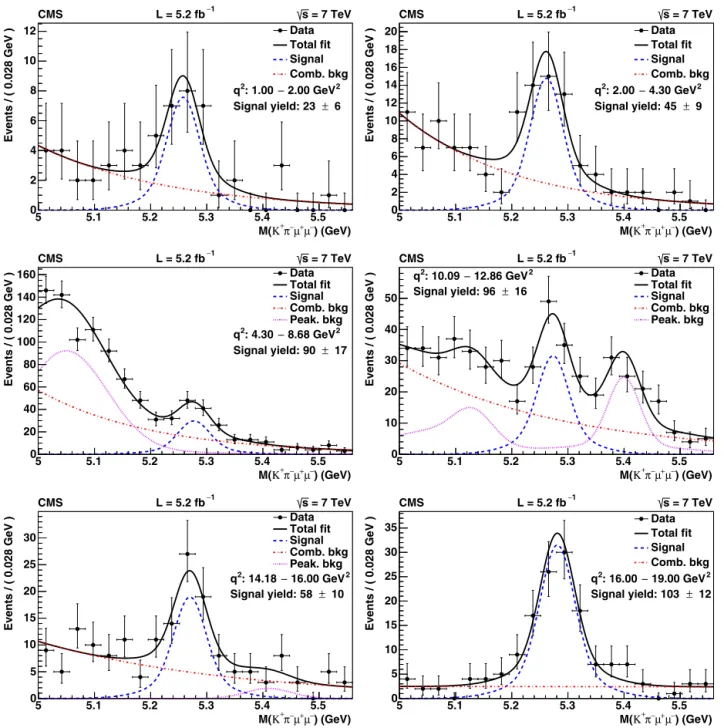
− are shown inFig. 3, along with the projection of the unbinned maximum-likelihood fit de-scribed in Section4. Clear signals are seen in each bin, with yields ranging from 23±
6 to 103±
12 events. The fitted results for FL and AFB are shown in Fig. 4, along with the SM predictions. The values of AFBand FL obtained for the firstq2bin are at the phys-ical boundary, which is enforced by a penalty term. This leads to statistical uncertainties, obtained fromminos[49], of zero for thepositive (negative) uncertainty for FL
(
AFB)
.The SM predictions are taken from Ref.[14]and combines two calculational techniques. In the low-q2 region, a QCD factorization approach[10]is used, which is applicable forq2
<
4m4c, wheremc is the charm quark mass. In the high-q2 region, an operator prod-uct expansion in the inverse b-quark mass and 1/
q2 [50,51] is combined with heavy quark form factor relations[52]. This is valid above the open-charm threshold. In both regions, the form factor calculations are taken from Ref.[53], and a dimensional estimate is made of the uncertainty from the expansion corrections [27]. Other recent SM calculations[15,17–19]give similar results, with the largest variations found in the uncertainty estimates and the differential branching fraction value. Between the J/ψ
andψ
′ res-onances, reliable theoretical predictions are not available.Using the efficiency corrected yields for the signal and normal-ization modes (B0
→
K∗0μ
+μ
− and B0→
K∗0J/ψ
) and the world-average branching fraction for the normalization mode [41], the branching fraction for B0→
K∗0μ
+μ
− is obtained as a function ofq2, as shown in Fig. 5, together with the SM predictions. The results forAFB, FL, and dB
/
dq2 are also reported inTable 2.The angular observables can be theoretically predicted with good control of the relevant form-factor uncertainties in the low dimuon invariant-mass region. It is therefore interesting to per-form the measurements of the relevant observables in the 1
<
q2<
6 GeV2 region. The experimental results in this region, along with the fit projections, are shown inFig. 6. The values obtained from this fit for FL, AFB, and dB
/
dq2 are shown in the bottom row of Table 2. These results are consistent with the SM pre-dictions of FL=
0.
74+0.06−0.07, AFB
= −
0.
05±
0.
03, and dB
/
dq2=
(
4.
9+1.0−1.1
)
×
10−8 GeV−2 [54].The results ofAFB,FL, and the branching fraction versusq2 are compared to previous measurements that use the same q2
bin-Fig. 2.The K+π−μ+μ− invariant-mass (top), cosθl (middle), and cosθK(bottom)
distributions for theq2bin associated with the B0→K∗0J/ψdecay, along with
re-sults from the projections of the overall unbinned maximum-likelihood fit (solid line), the signal contribution (dashed line), and the background contribution (dot-dashed line).
ning [36–38,55,56] in Fig. 7. The CMS measurements are more precise than all but the LHCb values, and in the highest-q2 bin, the CMS measurements have the smallest uncertainty in AFB and FL. Table 3provides a comparison of the same quantities in the low dimuon invariant-mass region: 1
<
q2<
6 GeV2.7. Summary
Using a data sample recorded with the CMS detector during 2011 and corresponding to an integrated luminosity of 5
.
2 fb−1, an angular analysis of the decay B0→
K∗0μ
+μ
−has been carried out. The data used for this analysis include more than 400 signal de-cays and 50 000 normalization/control mode dede-cays (B0→
K∗0J/ψ
and B0
Fig. 3.The K+π−μ+μ−invariant-mass distributions for each of the signalq2bins. Overlaid on each mass distribution is the projection of the unbinned maximum-likelihood
fit results for the overall fit (solid line), the signal contribution (dashed line), the combinatorial background contribution (dot-dashed line), and the peaking background contribution (dotted line).
Table 2
The yields and the measurements ofFL,AFB, and the branching fraction for the decay B0→K∗0μ+μ−in bins ofq2. The first uncertainty is statistical and the second is
systematic.
q2
(GeV2) Yield FL AFB d
B/dq2 (10−8GeV−2)
1–2 23.0±6.3 0.60+0.00
−0.28±0.19 −0.29+−00..3700±0.18 4.8+−11..42±0.4
2–4.3 45.0±8.8 0.65±0.17±0.03 −0.07±0.20±0.02 3.8±0.7±0.3
4.3–8.68 90±17 0.81+0.13
−0.12±0.05 −0.01±0.11±0.03 3.7±0.7±0.4
10.09–12.86 96±16 0.45+0.10
−0.11±0.04 0.40±0.08±0.05 5.4±0.9±0.9
14.18–16 58±10 0.53±0.12±0.03 0.29±0.09±0.05 4.6+0.9 −0.8±0.5
16–19 103±12 0.44±0.07±0.03 0.41±0.05±0.03 5.2±0.6±0.5
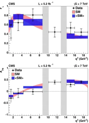
Fig. 4.Results of the measurement of FL (top) and AFB (bottom) versusq2. The
statistical uncertainty is shown by inner error bars, while the outer error bars give the total uncertainty. The vertical shaded regions correspond to the J/ψ and
ψ′resonances. The other shaded regions show the SM prediction as a continuous
distribution and after rate-averaging across theq2bins(SM)to allow direct
com-parison to the data points. Reliable theoretical predictions between the J/ψandψ′
resonances(10.09<q2<12.86 GeV2)are not available.
Fig. 5.Results of the measurement of dB/dq2versusq2. The statistical uncertainty
is shown by inner error bars, while the outer error bars give the total uncer-tainty. The vertical shaded regions correspond to the J/ψ andψ′ resonances. The
other shaded regions show the SM prediction as a continuous distribution and after rate-averaging across theq2 bins (SM)to allow direct comparison to the
data points. Reliable theoretical predictions between the J/ψ and ψ′ resonances
(10.09<q2<12.86 GeV2)are not available.
with three independent variables, the K+
π
−μ
+μ
−invariant mass and two decay angles, to obtain values of the forward–backward asymmetry of the muons,AFB, and the fraction of longitudinal po-larization of the K∗0,FL. Using these results, unbinned maximum-likelihood fits to the K+
π
−μ
+μ
− invariant mass inq2 bins have been used to extract the differential branching fraction dB
/
dq2. The results are consistent with the SM predictions and previousFig. 6. The K+π−μ+μ− invariant-mass (top), cosθl (middle), and cosθK
(bot-tom) distributions for 1<q2<6 GeV2, along with results from the projections of
the overall unbinned maximum-likelihood fit (solid line), the signal contribution (dashed line), and the background contribution (dot-dashed line).
measurements. Combined with other measurements, these results can be used to rule out or constrain new physics.
Acknowledgements
Fig. 7.Measurements versusq2ofFL(top),AFB(middle), and the branching fraction
(bottom) for B→K∗ℓ+ℓ−from CMS (this Letter), Belle[36], CDF[37,55], BaBar[56],
and LHCb[38]. The error bars give the total uncertainty. The vertical shaded regions correspond to the J/ψandψ′resonances. The other shaded regions are the result of rate-averaging the SM prediction across theq2bins to allow direct comparison to the data points. Reliable theoretical predictions between the J/ψandψ′resonances (10.09<q2<12.86 GeV2)are not available.
Table 3
Measurements from CMS (this Letter), LHCb [38], BaBar [56], CDF [37,55], and Belle[36]ofFL, AFB, and dB/dq2 in the region 1<q2<6 GeV2 for the decay
B→K∗ℓ+ℓ−. The first uncertainty is statistical and the second is systematic. The
SM predictions are also given[14].
Experiment FL AFB dB/dq2
(10−8GeV−2)
CMS 0.68±0.10±0.02 −0.07±0.12±0.01 4.4±0.6±0.4 LHCb 0.65+0.08
−0.07±0.03 −0.17±0.06±0.01 3.4±0.3+−00..45
BaBar – – 4.1+1.1
−1.0±0.1
CDF 0.69+0.19
−0.21±0.08 0.29−+00..2023±0.07 3.2±1.1±0.3
Belle 0.67±0.23±0.05 0.26+0.27
−0.32±0.07 3.0−+00..98±0.2
SM 0.74+0.06
−0.07 −0.05±0.03 4.9+−11..01
MES (Bulgaria); CERN; CAS, MoST, and NSFC (China); COLCIENCIAS (Colombia); MSES (Croatia); RPF (Cyprus); MoER, SF0690030s09 and ERDF (Estonia); Academy of Finland, MEC, and HIP (Finland); CEA and CNRS/IN2P3 (France); BMBF, DFG, and HGF (Germany); GSRT (Greece); OTKA and NKTH (Hungary); DAE and DST (India); IPM (Iran); SFI (Ireland); INFN (Italy); NRF and WCU (Republic of Korea); LAS (Lithuania); CINVESTAV, CONACYT, SEP, and UASLP-FAI (Mexico); MBIE (New Zealand); PAEC (Pakistan); MSHE and NSC (Poland); FCT (Portugal); JINR (Dubna); MON, RosAtom, RAS and RFBR (Russia); MESTD (Serbia); SEIDI and CPAN (Spain); Swiss Funding Agencies (Switzerland); NSC (Taipei); ThEPCenter, IPST, STAR and NSTDA (Thailand); TUBITAK and TAEK (Turkey); NASU (Ukraine); STFC (United Kingdom); DOE and NSF (USA).
Individuals have received support from the Marie-Curie pro-gramme and the European Research Council and EPLANET (Eu-ropean Union); the Leventis Foundation; the A.P. Sloan Founda-tion; the Alexander von Humboldt FoundaFounda-tion; the Belgian Fed-eral Science Policy Office; the Fonds pour la Formation à la Recherche dans l’Industrie et dans l’Agriculture (FRIA–Belgium); the Agentschap voor Innovatie door Wetenschap en Technolo-gie (IWT–Belgium); the Ministry of Education, Youth and Sports (MEYS) of Czech Republic; the Council of Science and Industrial Research, India; the Compagnia di San Paolo (Torino); the HOM-ING PLUS programme of Foundation for Polish Science, cofinanced by EU, Regional Development Fund; and the Thalis and Aristeia programmes cofinanced by EU–ESF and the Greek NSRF.
Open access
This article is published Open Access at sciencedirect.com. It is distributed under the terms of the Creative Commons Attribu-tion License 3.0, which permits unrestricted use, distribuAttribu-tion, and reproduction in any medium, provided the original authors and source are credited.
References
[1]N.G. Deshpande, J. Trampetic, Improved estimates for processesb→sℓ+ℓ−, B→Kℓ+ℓ−, andB→K∗ℓ+ℓ−, Phys. Rev. Lett. 60 (1988) 2583.
[2]N.G. Deshpande, Josip Trampetic, Kuriakose Panose, Resonance background to the decaysb→sℓ+ℓ−,B→K∗ℓ+ℓ−, andB→Kℓ+ℓ−, Phys. Rev. D 39 (1989)
1461.
[3]C.S. Lim, T. Morozumi, A.I. Sanda, A prediction for dΓ (b→sℓℓ)/dq2including the long-distance effects, Phys. Lett. B 218 (1989) 343.
[4]Benjamin Grinstein, Martin J. Savage, Mark B. Wise, B→Xse+e− in the six quark model, Nucl. Phys. B 319 (1989) 271.
[5]Ahmed Ali, T. Mannel, T. Morozumi, Forward backward asymmetry of dilepton angular distribution in the decayb→sℓ+ℓ−, Phys. Lett. B 273 (1991) 505. [6] Frank Krüger, Lalit M. Sehgal, Nita Sinha, Rahul Sinha, Angular distribution and
CP asymmetries in the decays B→K−π+e−e+and B→π−π+e−e+, Phys.
Rev. D 61 (2000) 114028,http://dx.doi.org/10.1103/PhysRevD.61.114028 (Erra-tum,http://dx.doi.org/10.1103/PhysRevD.63.019901).
[7]C.S. Kim, Yeong Gyun Kim, Cai-Dian Lu, Takuya Morozumi, Azimuthal angle distribution inB→K∗(→Kπ)ℓ+ℓ−at low invariantmℓ+ℓ−region, Phys. Rev.
D 62 (2000) 034013.
[8]Qi-Shu Yan, Chao-Shang Huang, Wei Liao, Shou-Hua Zhu, Exclusive semilep-tonic rare decaysB→(K,K∗)ℓ+ℓ−in supersymmetric theories, Phys. Rev. D
62 (2000) 094023.
[9]T.M. Aliev, A. Ozpineci, M. Savci, ExclusiveB→K∗ℓ+ℓ−decay with polarized
K∗and new physics effects, Phys. Lett. B 511 (2001) 49.
[10]M. Beneke, Th. Feldmann, D. Seidel, Systematic approach to exclusive B→ Vℓ+ℓ−,Vγdecays, Nucl. Phys. B 612 (2001) 25.
[11]Chuan-Hung Chen, C.Q. Geng, Probing new physics inB→K(∗)ℓ+ℓ−decays, Phys. Rev. D 66 (2002) 094018.
[12] Christoph Bobeth, Gudrun Hiller, Danny van Dyk, The benefits ofB→K∗ℓ+ℓ−
decays at low recoil, J. High Energy Phys. 1007 (2010) 098,http://dx.doi.org/ 10.1007/JHEP07(2010)098.
[14] Christoph Bobeth, Gudrun Hiller, Danny van Dyk, General analysis of B→ K(∗)ℓ+ℓ−decays at low recoil, Phys. Rev. D 87 (2012) 034016,http://dx.doi.org/
10.1103/PhysRevD.87.034016.
[15]A. Ali, G. Kramer, Guohuai Zhu,B→K∗ℓ+ℓ−decay in soft-collinear effective
theory, Eur. Phys. J. C 47 (2006) 625.
[16]Wolfgang Altmannshofer, Patricia Ball, Aoife Bharucha, Andrzej J. Buras, David M. Straub, Michael Wick, Symmetries and asymmetries ofB→K∗μ+μ−
de-cays in the Standard Model and beyond, J. High Energy Phys. 0901 (2009) 019.
[17] Wolfgang Altmannshofer, Paride Paradisi, David M. Straub, Model-independent constraints on new physics inb→stransitions, J. High Energy Phys. 1204 (2012) 008,http://dx.doi.org/10.1088/1126-6708/2009/01/019.
[18] S. Jäger, J. Martin Camalich, OnB→Vℓℓ at small dilepton invariant mass, power corrections, and new physics, J. High Energy Phys. 1305 (2013) 043, http://dx.doi.org/10.1007/JHEP05(2013)043.
[19]Sebastien Descotes-Genon, Tobias Hurth, Joaquim Matias, Javier Virto, Optimiz-ing the basis ofB→K∗ℓ+ℓ− observables in the full kinematic range, J. High
Energy Phys. 1305 (2013) 137.
[20]D. Melikhov, N. Nikitin, S. Simula, Probing right-handed currents in B→K∗ℓ+ℓ−transitions, Phys. Lett. B 442 (1998) 381.
[21]Ahmed Ali, Patricia Ball, L.T. Handoko, G. Hiller, A comparative study of the de-caysB→(K K∗)ℓ+ℓ−in standard model and supersymmetric theories, Phys.
Rev. D 61 (2000) 074024.
[22]Gerhard Buchalla, Gudrun Hiller, Gino Isidori, Phenomenology of nonstandard Zcouplings in exclusive semileptonicb→stransitions, Phys. Rev. D 63 (2000) 014015.
[23]Thorsten Feldmann, Joaquim Matias, Forward backward and isospin asymme-try forB→K∗ℓ+ℓ−decay in the standard model and in supersymmetry, J. High Energy Phys. 0301 (2003) 074.
[24]Gudrun Hiller, Frank Krüger, More model-independent analysis of b→s processes, Phys. Rev. D 69 (2004) 074020.
[25]Frank Krüger, Joaquim Matias, Probing new physics via the transverse am-plitudes ofB0→K∗0(→K−π+)ℓ+ℓ− at large recoil, Phys. Rev. D 71 (2005) 094009.
[26] Artyom Hovhannisyan, Wei-Shu Hou, Namit Mahajan,B→K∗ℓ+ℓ− forward–
backward asymmetry and new physics, Phys. Rev. D 77 (2008) 014016, http://dx.doi.org/10.1103/PhysRevD.77.014016.
[27]Ulrik Egede, Tobias Hurth, Joaquim Matias, Marc Ramon, Will Reece, New ob-servables in the decay modeBd→K∗0ℓ+ℓ−, J. High Energy Phys. 0811 (2008) 032.
[28]Tobias Hurth, Gino Isidori, Jernej F. Kamenik, Federico Mescia, Constraints on new physics in MFV models: A model-independent analysis of F=1 processes, Nucl. Phys. B 808 (2009) 326.
[29] Ashutosh Kumar Alok, Amol Dighe, Diptimoy Ghosh, David London, Joaquim Matias, Makiko Nagashima, Alejandro Szynkman, New-physics contributions to the forward–backward asymmetry inB→K∗μ+μ−, J. High Energy Phys.
1002 (2010) 053,http://dx.doi.org/10.1007/JHEP02(2010)053.
[30] Ashutosh Kumar Alok, Alakabha Datta, Amol Dighe, Murugeswaran Duraisamy, Diptimoy Ghosh, David London, New physics inb→sμ+μ−: CP-conserving
observables, J. High Energy Phys. 1111 (2011) 121,http://dx.doi.org/10.1007/ JHEP11(2011)121.
[31] Qin Chang, Xin-Qiang Li, Ya-Dong Yang, B→K∗ℓ+ℓ−, Kℓ+ℓ− decays in a family non-universalZ′model, J. High Energy Phys. 1004 (2010) 052,http:// dx.doi.org/10.1007/JHEP04(2010)052.
[32] Sebastien Descotes-Genon, Diptimoy Ghosh, Joaquim Matias, Marc Ramon, Ex-ploring new physics in the C7–C7′ plane, J. High Energy Phys. 1106 (2011)
099,http://dx.doi.org/10.1007/JHEP06(2011)099.
[33]Joaquim Matias, Federico Mescia, Marc Ramon, Javier Virto, Complete anatomy of Bd→K∗0(→Kπ)ℓ+ℓ− and its angular distribution, J. High Energy Phys. 1204 (2012) 104.
[34] Sebastien Descotes-Genon, Joaquim Matias, Marc Ramon, Javier Virto, Impli-cations from clean observables for the binned analysis of B→K∗μ+μ− at
large recoil, J. High Energy Phys. 1301 (2013) 048,http://dx.doi.org/10.1007/ JHEP01(2013)048.
[35]Bernard Aubert, et al., Angular distributions in the decayB→K∗ℓ+ℓ−, Phys. Rev. D 79 (2009) 031102.
[36]J.-T. Wei, et al., Measurement of the differential branching fraction and forward–backward asymmetry for B→K(∗)ℓ+ℓ−, Phys. Rev. Lett. 103 (2009)
171801.
[37]T. Aaltonen, et al., Measurements of the angular distributions in the decays B→K(∗)μ+μ−at CDF, Phys. Rev. Lett. 108 (2012) 081807.
[38]R. Aaij, et al., Differential branching fraction and angular analysis of the decay B0→K∗0μ+μ−, J. High Energy Phys. 1308 (2013) 131.
[39] CMS Collaboration, CMS luminosity based on pixel cluster counting – summer 2013 update, CMS Physics Analysis Summary CMS-PAS-LUM-13–001, 2013, http://cds.cern.ch/record/1598864.
[40] S. Chatrchyan, et al., The CMS experiment at the CERN LHC, JINST 3 (2008) S08004,http://dx.doi.org/10.1088/1748-0221/3/08/S08004.
[41]Particle Data Group, J. Beringer, et al., Review of particle physics, Phys. Rev. D 86 (2012) 010001. See also the 2013 partial update for the 2014 edition. [42]Torbjörn Sjöstrand, Stephen Mrenna, Peter Skands, PYTHIA 6.4 physics and
manual, J. High Energy Phys. 0605 (2006) 026.
[43]D.J. Lange, The EvtGen particle decay simulation package, Nucl. Instrum. Methods A 462 (2001) 152.
[44]S. Agostinelli, et al., Geant4 – a simulation toolkit, Nucl. Instrum. Methods A 506 (2003) 250.
[45]Damir Becirevic, Andrey Tayduganov, Impact of B→K∗0ℓ+ℓ− on the new
physics search inB→K∗ℓ+ℓ−decay, Nucl. Phys. B 868 (2013) 368.
[46]Joaquim Matias, On the S-wave pollution of B→K∗ℓ+ℓ− observables, Phys.
Rev. D 86 (2012) 094024.
[47] Thomas Blake, Ulrik Egede, Alex Shires, The effect ofS-wave interference on theB0→K∗0ℓ+ℓ−angular observables, J. High Energy Phys. 1303 (2013) 027,
http://dx.doi.org/10.1007/JHEP03(2013)027.
[48]R. Aaij, et al., Measurement of relative branching fractions of B decays to
ψ (2S)and J/ψmesons, Eur. Phys. J. C 72 (2012) 2118.
[49]F. James, M. Roos, Minuit – a system for function minimization and analysis of the parameter errors and correlations, Comput. Phys. Commun. 10 (1975) 343. [50] Benjamin Grinstein, Dan Pirjol, Exclusive rare B→K∗ℓ+ℓ− decays at low recoil: controlling the long-distance effects, Phys. Rev. D 70 (2004) 114005, http://dx.doi.org/10.1103/PhysRevD.70.114005.
[51]M. Beylich, G. Buchalla, T. Feldmann, Theory ofB→K(∗)ℓ+ℓ−decays at high
q2: OPE and quark–hadron duality, Eur. Phys. J. C 71 (2011) 1635.
[52] Benjamin Grinstein, Dan Pirjol, Symmetry-breaking corrections to heavy meson form-factor relations, Phys. Lett. B 533 (8) (2002), http://dx.doi.org/10.1016/ S0370-2693(02)01601-5.
[53]Patricia Ball, Roman Zwicky, Bd,s→ρ, ω,K∗, φ decay form factors from light-cone sum rules reexamined, Phys. Rev. D 71 (2005) 014029.
[54] Christoph Bobeth, Gudrun Hiller, Danny van Dyk, More benefits of semilep-tonic rare b decays at low recoil: CP violation, J. High Energy Phys. 1107 (2011) 067,http://dx.doi.org/10.1007/JHEP07(2011)067.
[55]T. Aaltonen, et al., Measurement of the forward–backward asymmetry in the B→K(∗)μ+μ−decay and first observation of theB0s→φμ+μ−decay, Phys. Rev. Lett. 106 (2011) 161801.
[56]J.P. Lees, et al., Measurement of branching fractions and rate asymmetries in the rare decaysB→K(∗)ℓ+ℓ−, Phys. Rev. D 86 (2012) 032012.
CMS Collaboration
S. Chatrchyan, V. Khachatryan, A.M. Sirunyan, A. Tumasyan
Yerevan Physics Institute, Yerevan, Armenia
W. Adam, T. Bergauer, M. Dragicevic, J. Erö, C. Fabjan
1, M. Friedl, R. Frühwirth
1, V.M. Ghete,
N. Hörmann, J. Hrubec, M. Jeitler
1, W. Kiesenhofer, V. Knünz, M. Krammer
1, I. Krätschmer, D. Liko,
I. Mikulec, D. Rabady
2, B. Rahbaran, C. Rohringer, H. Rohringer, R. Schöfbeck, J. Strauss, A. Taurok,
W. Treberer-Treberspurg, W. Waltenberger, C.-E. Wulz
1Institut für Hochenergiephysik der OeAW, Wien, Austria
National Centre for Particle and High Energy Physics, Minsk, Belarus
S. Alderweireldt, M. Bansal, S. Bansal, T. Cornelis, E.A. De Wolf, X. Janssen, A. Knutsson, S. Luyckx,
L. Mucibello, S. Ochesanu, B. Roland, R. Rougny, Z. Staykova, H. Van Haevermaet, P. Van Mechelen,
N. Van Remortel, A. Van Spilbeeck
Universiteit Antwerpen, Antwerpen, Belgium
F. Blekman, S. Blyweert, J. D’Hondt, A. Kalogeropoulos, J. Keaveney, M. Maes, A. Olbrechts, S. Tavernier,
W. Van Doninck, P. Van Mulders, G.P. Van Onsem, I. Villella
Vrije Universiteit Brussel, Brussel, Belgium
C. Caillol, B. Clerbaux, G. De Lentdecker, L. Favart, A.P.R. Gay, T. Hreus, A. Léonard, P.E. Marage,
A. Mohammadi, L. Perniè, T. Reis, T. Seva, L. Thomas, C. Vander Velde, P. Vanlaer, J. Wang
Université Libre de Bruxelles, Bruxelles, Belgium
V. Adler, K. Beernaert, L. Benucci, A. Cimmino, S. Costantini, S. Dildick, G. Garcia, B. Klein, J. Lellouch,
A. Marinov, J. Mccartin, A.A. Ocampo Rios, D. Ryckbosch, M. Sigamani, N. Strobbe, F. Thyssen, M. Tytgat,
S. Walsh, E. Yazgan, N. Zaganidis
Ghent University, Ghent, Belgium
S. Basegmez, C. Beluffi
3, G. Bruno, R. Castello, A. Caudron, L. Ceard, G.G. Da Silveira, C. Delaere,
T. du Pree, D. Favart, L. Forthomme, A. Giammanco
4, J. Hollar, P. Jez, V. Lemaitre, J. Liao, O. Militaru,
C. Nuttens, D. Pagano, A. Pin, K. Piotrzkowski, A. Popov
5, M. Selvaggi, J.M. Vizan Garcia
Université Catholique de Louvain, Louvain-la-Neuve, Belgium
N. Beliy, T. Caebergs, E. Daubie, G.H. Hammad
Université de Mons, Mons, Belgium
G.A. Alves, M. Correa Martins Junior, T. Martins, M.E. Pol, M.H.G. Souza
Centro Brasileiro de Pesquisas Fisicas, Rio de Janeiro, Brazil
W.L. Aldá Júnior, W. Carvalho, J. Chinellato
6, A. Custódio, E.M. Da Costa, D. De Jesus Damiao,
C. De Oliveira Martins, S. Fonseca De Souza, H. Malbouisson, M. Malek, D. Matos Figueiredo, L. Mundim,
H. Nogima, W.L. Prado Da Silva, A. Santoro, A. Sznajder, E.J. Tonelli Manganote
6, A. Vilela Pereira
Universidade do Estado do Rio de Janeiro, Rio de Janeiro, Brazil
C.A. Bernardes
b, F.A. Dias
a,
7, T.R. Fernandez Perez Tomei
a, E.M. Gregores
b, C. Lagana
a,
P.G. Mercadante
b, S.F. Novaes
a, Sandra S. Padula
a aUniversidade Estadual Paulista, São Paulo, BrazilbUniversidade Federal do ABC, São Paulo, Brazil
V. Genchev
2, P. Iaydjiev
2, S. Piperov, M. Rodozov, G. Sultanov, M. Vutova
Institute for Nuclear Research and Nuclear Energy, Sofia, Bulgaria
A. Dimitrov, R. Hadjiiska, V. Kozhuharov, L. Litov, B. Pavlov, P. Petkov
University of Sofia, Sofia, Bulgaria
J.G. Bian, G.M. Chen, H.S. Chen, C.H. Jiang, D. Liang, S. Liang, X. Meng, J. Tao, X. Wang, Z. Wang, H. Xiao
Institute of High Energy Physics, Beijing, China
C. Asawatangtrakuldee, Y. Ban, Y. Guo, W. Li, S. Liu, Y. Mao, S.J. Qian, H. Teng, D. Wang, L. Zhang, W. Zou
C. Avila, C.A. Carrillo Montoya, L.F. Chaparro Sierra, J.P. Gomez, B. Gomez Moreno, J.C. Sanabria
Universidad de Los Andes, Bogota, Colombia
N. Godinovic, D. Lelas, R. Plestina
8, D. Polic, I. Puljak
Technical University of Split, Split, Croatia
Z. Antunovic, M. Kovac
University of Split, Split, Croatia
V. Brigljevic, K. Kadija, J. Luetic, D. Mekterovic, S. Morovic, L. Tikvica
Institute Rudjer Boskovic, Zagreb, Croatia
A. Attikis, G. Mavromanolakis, J. Mousa, C. Nicolaou, F. Ptochos, P.A. Razis
University of Cyprus, Nicosia, Cyprus
M. Finger, M. Finger Jr.
Charles University, Prague, Czech Republic
A.A. Abdelalim
9, Y. Assran
10, S. Elgammal
9, A. Ellithi Kamel
11, M.A. Mahmoud
12, A. Radi
13,
14Academy of Scientific Research and Technology of the Arab Republic of Egypt, Egyptian Network of High Energy Physics, Cairo, Egypt
M. Kadastik, M. Müntel, M. Murumaa, M. Raidal, L. Rebane, A. Tiko
National Institute of Chemical Physics and Biophysics, Tallinn, Estonia
P. Eerola, G. Fedi, M. Voutilainen
Department of Physics, University of Helsinki, Helsinki, Finland
J. Härkönen, V. Karimäki, R. Kinnunen, M.J. Kortelainen, T. Lampén, K. Lassila-Perini, S. Lehti, T. Lindén,
P. Luukka, T. Mäenpää, T. Peltola, E. Tuominen, J. Tuominiemi, E. Tuovinen, L. Wendland
Helsinki Institute of Physics, Helsinki, Finland
T. Tuuva
Lappeenranta University of Technology, Lappeenranta, Finland
M. Besancon, F. Couderc, M. Dejardin, D. Denegri, B. Fabbro, J.L. Faure, F. Ferri, S. Ganjour, A. Givernaud,
P. Gras, G. Hamel de Monchenault, P. Jarry, E. Locci, J. Malcles, L. Millischer, A. Nayak, J. Rander,
A. Rosowsky, M. Titov
DSM/IRFU, CEA/Saclay, Gif-sur-Yvette, France
S. Baffioni, F. Beaudette, L. Benhabib, M. Bluj
15, P. Busson, C. Charlot, N. Daci, T. Dahms, M. Dalchenko,
L. Dobrzynski, A. Florent, R. Granier de Cassagnac, M. Haguenauer, P. Miné, C. Mironov, I.N. Naranjo,
M. Nguyen, C. Ochando, P. Paganini, D. Sabes, R. Salerno, Y. Sirois, C. Veelken, A. Zabi
Laboratoire Leprince-Ringuet, Ecole Polytechnique, IN2P3-CNRS, Palaiseau, France
J.-L. Agram
16, J. Andrea, D. Bloch, J.-M. Brom, E.C. Chabert, C. Collard, E. Conte
16, F. Drouhin
16,
J.-C. Fontaine
16, D. Gelé, U. Goerlach, C. Goetzmann, P. Juillot, A.-C. Le Bihan, P. Van Hove
Institut Pluridisciplinaire Hubert Curien, Université de Strasbourg, Université de Haute Alsace Mulhouse, CNRS/IN2P3, Strasbourg, France
S. Gadrat
S. Beauceron, N. Beaupere, G. Boudoul, S. Brochet, J. Chasserat, R. Chierici, D. Contardo, P. Depasse,
H. El Mamouni, J. Fay, S. Gascon, M. Gouzevitch, B. Ille, T. Kurca, M. Lethuillier, L. Mirabito, S. Perries,
L. Sgandurra, V. Sordini, M. Vander Donckt, P. Verdier, S. Viret
Université de Lyon, Université Claude Bernard Lyon 1, CNRS-IN2P3, Institut de Physique Nucléaire de Lyon, Villeurbanne, France
Z. Tsamalaidze
17Institute of High Energy Physics and Informatization, Tbilisi State University, Tbilisi, Georgia
C. Autermann, S. Beranek, B. Calpas, M. Edelhoff, L. Feld, N. Heracleous, O. Hindrichs, K. Klein,
A. Ostapchuk, A. Perieanu, F. Raupach, J. Sammet, S. Schael, D. Sprenger, H. Weber, B. Wittmer,
V. Zhukov
5RWTH Aachen University, I. Physikalisches Institut, Aachen, Germany
M. Ata, J. Caudron, E. Dietz-Laursonn, D. Duchardt, M. Erdmann, R. Fischer, A. Güth, T. Hebbeker,
C. Heidemann, K. Hoepfner, D. Klingebiel, S. Knutzen, P. Kreuzer, M. Merschmeyer, A. Meyer,
M. Olschewski, K. Padeken, P. Papacz, H. Pieta, H. Reithler, S.A. Schmitz, L. Sonnenschein, J. Steggemann,
D. Teyssier, S. Thüer, M. Weber
RWTH Aachen University, III. Physikalisches Institut A, Aachen, Germany
V. Cherepanov, Y. Erdogan, G. Flügge, H. Geenen, M. Geisler, W. Haj Ahmad, F. Hoehle, B. Kargoll,
T. Kress, Y. Kuessel, J. Lingemann
2, A. Nowack, I.M. Nugent, L. Perchalla, O. Pooth, A. Stahl
RWTH Aachen University, III. Physikalisches Institut B, Aachen, Germany
I. Asin, N. Bartosik, J. Behr, W. Behrenhoff, U. Behrens, A.J. Bell, M. Bergholz
18, A. Bethani, K. Borras,
A. Burgmeier, A. Cakir, L. Calligaris, A. Campbell, S. Choudhury, F. Costanza, C. Diez Pardos, S. Dooling,
T. Dorland, G. Eckerlin, D. Eckstein, G. Flucke, A. Geiser, I. Glushkov, A. Grebenyuk, P. Gunnellini,
S. Habib, J. Hauk, G. Hellwig, D. Horton, H. Jung, M. Kasemann, P. Katsas, C. Kleinwort, H. Kluge,
M. Krämer, D. Krücker, E. Kuznetsova, W. Lange, J. Leonard, K. Lipka, W. Lohmann
18, B. Lutz, R. Mankel,
I. Marfin, I.-A. Melzer-Pellmann, A.B. Meyer, J. Mnich, A. Mussgiller, S. Naumann-Emme, O. Novgorodova,
F. Nowak, J. Olzem, H. Perrey, A. Petrukhin, D. Pitzl, R. Placakyte, A. Raspereza, P.M. Ribeiro Cipriano,
C. Riedl, E. Ron, M.Ö. Sahin, J. Salfeld-Nebgen, R. Schmidt
18, T. Schoerner-Sadenius, N. Sen, M. Stein,
R. Walsh, C. Wissing
Deutsches Elektronen-Synchrotron, Hamburg, Germany
M. Aldaya Martin, V. Blobel, H. Enderle, J. Erfle, E. Garutti, U. Gebbert, M. Görner, M. Gosselink, J. Haller,
K. Heine, R.S. Höing, G. Kaussen, H. Kirschenmann, R. Klanner, R. Kogler, J. Lange, I. Marchesini,
T. Peiffer, N. Pietsch, D. Rathjens, C. Sander, H. Schettler, P. Schleper, E. Schlieckau, A. Schmidt,
M. Schröder, T. Schum, M. Seidel, J. Sibille
19, V. Sola, H. Stadie, G. Steinbrück, J. Thomsen, D. Troendle,
E. Usai, L. Vanelderen
University of Hamburg, Hamburg, Germany
C. Barth, C. Baus, J. Berger, C. Böser, E. Butz, T. Chwalek, W. De Boer, A. Descroix, A. Dierlamm,
M. Feindt, M. Guthoff
2, F. Hartmann
2, T. Hauth
2, H. Held, K.H. Hoffmann, U. Husemann, I. Katkov
5,
J.R. Komaragiri, A. Kornmayer
2, P. Lobelle Pardo, D. Martschei, Th. Müller, M. Niegel, A. Nürnberg,
O. Oberst, J. Ott, G. Quast, K. Rabbertz, F. Ratnikov, S. Röcker, F.-P. Schilling, G. Schott, H.J. Simonis,
F.M. Stober, R. Ulrich, J. Wagner-Kuhr, S. Wayand, T. Weiler, M. Zeise
Institut für Experimentelle Kernphysik, Karlsruhe, Germany
G. Anagnostou, G. Daskalakis, T. Geralis, S. Kesisoglou, A. Kyriakis, D. Loukas, A. Markou, C. Markou,
E. Ntomari, I. Topsis-giotis
L. Gouskos, A. Panagiotou, N. Saoulidou, E. Stiliaris
University of Athens, Athens, Greece
X. Aslanoglou, I. Evangelou, G. Flouris, C. Foudas, P. Kokkas, N. Manthos, I. Papadopoulos, E. Paradas
University of Ioánnina, Ioánnina, Greece
G. Bencze, C. Hajdu, P. Hidas, D. Horvath
20, F. Sikler, V. Veszpremi, G. Vesztergombi
21, A.J. Zsigmond
KFKI Research Institute for Particle and Nuclear Physics, Budapest, Hungary
N. Beni, S. Czellar, J. Molnar, J. Palinkas, Z. Szillasi
Institute of Nuclear Research ATOMKI, Debrecen, Hungary
J. Karancsi, P. Raics, Z.L. Trocsanyi, B. Ujvari
University of Debrecen, Debrecen, Hungary
S.K. Swain
22National Institute of Science Education and Research, Bhubaneswar, India
S.B. Beri, V. Bhatnagar, N. Dhingra, R. Gupta, M. Kaur, M.Z. Mehta, M. Mittal, N. Nishu, A. Sharma,
J.B. Singh
Panjab University, Chandigarh, India
Ashok Kumar, Arun Kumar, S. Ahuja, A. Bhardwaj, B.C. Choudhary, S. Malhotra, M. Naimuddin, K. Ranjan,
P. Saxena, V. Sharma, R.K. Shivpuri
University of Delhi, Delhi, India
S. Banerjee, S. Bhattacharya, K. Chatterjee, S. Dutta, B. Gomber, Sa. Jain, Sh. Jain, R. Khurana, A. Modak,
S. Mukherjee, D. Roy, S. Sarkar, M. Sharan, A.P. Singh
Saha Institute of Nuclear Physics, Kolkata, India
A. Abdulsalam, D. Dutta, S. Kailas, V. Kumar, A.K. Mohanty
2, L.M. Pant, P. Shukla, A. Topkar
Bhabha Atomic Research Centre, Mumbai, India
T. Aziz, R.M. Chatterjee, S. Ganguly, S. Ghosh, M. Guchait
23, A. Gurtu
24, G. Kole, S. Kumar, M. Maity
25,
G. Majumder, K. Mazumdar, G.B. Mohanty, B. Parida, K. Sudhakar, N. Wickramage
26Tata Institute of Fundamental Research – EHEP, Mumbai, India
S. Banerjee, S. Dugad
Tata Institute of Fundamental Research – HECR, Mumbai, India
H. Arfaei, H. Bakhshiansohi, S.M. Etesami
27, A. Fahim
28, A. Jafari, M. Khakzad,
M. Mohammadi Najafabadi, S. Paktinat Mehdiabadi, B. Safarzadeh
29, M. Zeinali
Institute for Research in Fundamental Sciences (IPM), Tehran, Iran
M. Grunewald
University College Dublin, Dublin, Ireland


![Fig. 7. Measurements versus q 2 of F L (top), A FB (middle), and the branching fraction (bottom) for B → K ∗ ℓ + ℓ − from CMS (this Letter), Belle [36], CDF [37,55], BaBar [56], and LHCb [38]](https://thumb-eu.123doks.com/thumbv2/123dok_br/15748895.126640/8.918.71.419.105.800/measurements-versus-middle-branching-fraction-letter-belle-babar.webp)
