Environmental Policy and Growth when
Inputs are Differentiated in Pollution Intensity
Francesco Ricci
∗ †25 November 2004
Abstract
Environmental policy affects the distribution of market shares if intermediate goods are differentiated in their pollution intensity. When innovations are environment-friendly, a tax on emissions skews demand towards new goods which are the most productive. In this case, the tax has to increase along a balanced growth path to keep the market shares of goods of different vintages constant. Comparing balanced growth paths, we find that an increase in the burden of environmental taxation spurs innovation because it increases the market share of recent vintages. As a result the cost of environmental policy in terms of slower growth is weaker and may even be absent.
Keywords: Endogenous growth; Environmental policy; Induced technological change
JEL Classification Codes: O41; Q28; H32; O30
∗THEMA - Universit´e de Cergy-Pontoise, and LERNA.
Address: THEMA, Universit´e de Cergy-Pontoise, 33 bd du Port, 95011 Cergy-Pontoise, France. Tel: +33 1 3425 6180; fax: +33 1 3425 6233; e-mail: francesco.ricci@eco.u-cergy.fr
†I am very grateful to Lucas Bretschger, Hippolyte d’Albis, Andr´e Grimaud, Peter Howitt, Paola
Peretti, Gilles Saint-Paul, Katheline Schubert, an anonymous referee and in particular to Fabrice Collard and Bertrand Villeneuve, for their helpful comments. Of course all remaining errors are mine.
1
Introduction
Production activities have grown so much that they now play a primary role in the func-tioning of the ecosystem. The conservation of the ecosystem may significantly constrain further expansion of economic activity. The case of global warming is particularly im-portant in the current international agenda of environmental policy. There is substantial agreement among the scientific community that climate change is exacerbated by emis-sions of green-house gases, such as methane and carbon dioxide (CO2). Carbon emissions result from burning fossil fuel, the main source of primary energy. With current tech-nology and equipment, a reduction in emissions requires a fall in energy inputs which is likely to lower output below its potential level. Emissions can be controlled by imposing a tax or a quota on emissions (supported for instance by a market for pollution permits). We define this policy a restrictive environmental policy.
For a positive analysis, a question arises:1 how does a restrictive environmental policy influence the prospects of economic growth? The answer is not so obvious as the one discussed above concerning the impact on current level of production. This is because technology and equipment change in the long run. In recent years a body of theoretical papers has addressed this question using endogenous growth models. In these analyses emissions are formalized as an input or a by-product. In any case environmental policy operates through adirect channel of transmission. It increases the cost of emission inputs or forces firms to engage in abatement expenditure and therefore reduces the return on capital. As a result, the rate of investment falls and this slows output growth rate. In short, there is a trade-off between economic growth and environmental quality protection.2 A number of analyses have explored the possibility that some other channels of trans-mission of environmental policy on growth can relax this trade-off. Within the class of one-sector growth models two main channels have been proposed. A first strand of papers examines how environmental policy affects growth through its influence on households’ saving behavior (e.g. Fisher and Marrewijk 1998). In particular, if consumption and environmental quality are complements, expected improvements in environmental quality induce households to save more and postpone consumption (Mohtadi 1996, Michel and Rotillon 1995). It is questionable though that environmental policy may play a primary role in the determination of households’ savings. A second approach assumes increasing
1
The question may not be relevant for the design of environmental policy, given that the latter should target social welfare. Yet the answer is interesting on its own, at least in view of governments’ reluctance to engage in stringent targets for the reduction of CO2emissions.
2
returns in pollution abatement, and finds that growth makes it possible to increase the efficiency of abatement activities (Michel 1993, Xepapadeas 1994, Andreoni and Levin-son 2001). Within the class of multi-sector growth models instead two arguments have been put forward to justify positive channels of transmission of environmental policy on growth. On the one hand, improvements in environmental quality may enhance either total factor productivity or productivity in the core sector for growth, such as human capital accumulation.3 These assumptions seem plausible for economies that rely heav-ily on the exploitation of natural resources or economies where pollution is so serious as to weaken pupils’cognitive ability. In the case of most industrialized economies it is debatable whether improvements in the quality of the environment can have first order effects on factors’ productivity. On the other hand, some authors argue that environ-mental policy entails a reallocation of resources out of the production sector and into the dynamic sector of the economy, which may result in faster growth. Environmental policy may then foster human capital accumulation, as in Hettich (1998), or R&D activity as in Elbasha and Roe (1996) or Bretschger (1998). Our contribution adds to the latter strand of literature. For a survey of these approaches see Ricci (2004).
This paper provides the rationale for an alternative channel of transmission of environ-mental policy on growth which tends to relax the trade-off between environenviron-mental quality protection and economic growth. The theory presented in the following pages gives struc-ture to the statement “environmental policy fosters innovations and can therefore promote growth, regardless of any productive or amenity role of environmental quality”. In order to sharpen the argument we deliberately abstract from the functioning of the ecosystem, and from the influence of environmental quality or pollution on welfare and on factors’ productivity. As a result, our analysis does not include any normative justification for environmental policy. This feature is meant to strengthen our argument and to single out its originality: the independence of the transmission channel from any externality result-ing from improvements in environmental quality. The analysis can easily be generalized to include welfare considerations for normative enquiry.4
This paper builds on the Schumpeterian growth theory, which explicitly models in-centives to engage in productivity enhancing activities (hereafter R&D) (Grossman and
3
See e.g. Bovenberg and Smulders 1995, Smulders and Gradus 1996, Gradus and Smulders 1993.
4
Helpman 1991, Aghion and Howitt 1992).5 It is assumed that innovations improve the quality of capital goods in two dimensions: their productivity and their pollution inten-sity. New goods are characterized by higher productivity and, possibly, lower pollution intensity than existing goods.6 If innovations embody the same pollution intensity as the goods they replace, emissions grow at the same rate as output. If instead innovations have a cleaner technology, emissions grow at a slower rate than output. The flow of services that capital goods provide are called intermediate goods. Their operating cost is com-posed of the rental rate of capital and the tax on emissions associated with their use. The relative weight of these components can be managed by the environmental policy-maker and affects incentives to invest and the pace of growth if it varies across vintages. The next section presents the model, while section 3 characterizes balanced growth paths.
In section 4, we analyze the case where the extent to which innovations are cleaner is exogenous, and in particular independent of environmental policy. This assumption allows us to focus on the description of an original channel of transmission through which environmental policy affects the pace of technological change and the rate of growth. We show that a tax on emissions has a distortionary impact on competition across sectors, when goods are differentiated in their pollution intensity. To the extent that there is a (negative) correlation between the productivity of goods and their pollution intensity, tax on emissions acts as a (relative) reward to innovators. In fact, tax on emissions increase the market share of the newer and more productive goods and increase the relative pay-off to R&D investment. We find that when goods are differentiated in emission intensity, an increase in the burden of emissions taxes raises the long-run rate of growth by fostering R&D activity, even though - on impact - it may reduce the level of aggregate output.
Our argument is close to Xepapadeas and de Zeeuw (1999) and Feichtinger et al. (2004), who analyze a single firm’s choice of the vintage composition of its capital stock. They show that an increase in emissions taxes induces firms to reduce the average age of their capital stock, and identify the conditions under which this response implies higher productivity of capital. The theory presented in the following sections incorporates this mechanism in a dynamic general equilibrium model, where the supply-of-capital side of the economy is endogenous in both its quality (designs of innovations) and quantity
(saving-5
Our model is an extension of Aghion and Howitt’s (1998, p.85-92). As explained in Ricci (2002), the Aghion-Howitt framework is the only dynamic general equilibrium model where the degree of hetero-geneity of profits across sectors is endogenously determined. This feature is crucial for our results.
6
investment decision) dimensions. Our model nevertheless is simpler in some respects, namely in assuming that capital is putty-putty while only technologies are putty-clay.
Section 5 considers the case where R&D laboratories choose endogenously the pol-lution intensity of innovations. Here environmental policy affects the extent to which innovations embody cleaner technologies, i.e. thedirection of R&D.7 In this way we rein-troduce the possibility that environmental policy has a negative impact on growth. In fact, emissions are an implicit input of production. Cleaner innovations are relatively less productive, because they use a smaller amount of the complementary emissions input. Hence, as environmental policy induces R&D laboratories to design cleaner goods, the marginal effect of R&D on productivity growth decreases. This direct input effect runs in a direction opposite to the one resulting from the distortionary impact of emissions taxes (which tends to foster R&D). Solving the model numerically, we find that the direct effect dominates. However, the distortionary impact of taxation is active and relaxes the growth-environment trade-off.
The analysis by Hart (2004 a) is very close to ours. Similarly, it builds on the Aghion-Howitt framework where environmental policy heterogeneously affects profits across vin-tages, if these embody different pollution intensity technologies. Unlike in our case, at-tention is restricted to state contingent technology standards, implying an exogenously determined maximum age of equipment in use.8 Also analytical results are obtained un-der a simplifying assumption: R&D labs are constrained to choose their technology out of a discrete two-point set. Because of this rigidity, the direct input effect may be weak enough for the distortionary effect to dominate, giving rise to a win-win outcome with en-vironmental policy improving both growth rate and enen-vironmental quality. We find that this result is not robust to an increase in flexibility in R&D labs’ technological choice.
We first present the model and its balanced growth properties. Next we analyze the consequences of tightening environmental policy on innovation, direction of technological change and growth rate.
2
The model economy
We extend the Schumpeterian model of endogenous growth (like that of Aghion and Howitt 1998, p.85-92) to consider that production emits pollutants. Production takes
7
See Popp (2002) and Jaffe et al. (2002) for relevant empirical evidence.
8
place in three stages. First, labor is competitively engaged in research and development (R&D) activities aimed at designing higher-quality intermediate goods. Successful inno-vations are characterized by higher productivity and, possibly, lower pollution intensity. Pollution intensity is a technological variable of the intermediate good, which is chosen by the R&D laboratory when it introduces the good on the market. This choice is irreversible and a lower pollution intensity implies a lower productivity of the good. Second, designs are protected by patents, so that intermediate goods are supplied under local monopoly power. These goods are produced employing capital. Their production also implies emis-sions of pollution. We assume a continuum of intermediate goods. Producers rent capital from households and pay a tax per unit of emissions resulting from their activities. Third, intermediate goods are combined with labor in the final sector to produce a homogeneous good which can be consumed or invested.
In this section we first present the production functions of the final and intermediate sectors, and emissions. Next we study the behavior of the agents: the final sector, a repre-sentative intermediate good monopolist, the R&D sector, consumers and the government.
2.1
Production and the environment
Final output is produced employing labor and a continuum of intermediate inputs accord-ing to the production function:
Yτ = (1−nτ)1−α
Z 1
0
ZjτAjτxαjτdj (1)
where α ∈ (0,1); labor supply is fixed and normalized to unit mass; a share (1−n) of labor is employed in production and n in R&D activities (if the labor market clears);xjτ
is the quantity of intermediate goodj ∈[0,1] used at dateτ. The technology embodied in intermediate goods is described by a two-dimensional vector characterized by parameters
A and Z. Ajτ is the implicit labor productivity index and Zjτ the pollution intensity
index of intermediate good j at date τ. As shown in the production function (1), the productivity of good j at date τ depends on the product ZjτAjτ. These definitions and
the link between parameterZ and productivity are explained at the end of this subsection. Intermediate goods are produced employing capital, according to:
xjτ =
Kjτ
Ajτ
Thus, intermediate goods are services from capital goods, and the more productive the good the higher its capital intensity.9
The flow of emissions, Pjτ, associated with the use of a capital good depends on its
pollution intensity index at date τ, Zjτ, and is given by, ∀ j ∈[0,1]:
Pjτ =Zjτ1/αβKjτ (3)
with β∈(0,1). Thus aggregate emissions, P, can be defined as follows:
Pτ =
Z 1
0
Pjτdj =
Z 1
0
Zjτ1/αβKjτdj (4)
SubstitutingKjτ in (2) using (3), we see that good j is produced out of emissions:
xjτ =
Pjτ
Zjτ1/αβAjτ
.
(3) can be written as:
Zjτ =
µ Pjτ
Kjτ
¶αβ
Thus Zjτ is a measure of the emissions-capital ratio characteristic of good j at date τ.
For a given technology Zj, the substitution of capital for emissions cannot take place,
e.g. in response to a shift in their relative price. Substitution can take place only with the introduction of a new technology in sectorj, say Z′
j. Pollution intensity is reduced if
the new technology satisfies Z′
j < Zj. A new technology can be introduced only through
R&D. At the industry level, substitution is therefore costly and discontinuous over time. Emissions are implicit inputs that are combined with intermediate inputs according to their pollution intensity. SubstitutingZjτ above and xjτ in (1) using (2), we get:
Yτ =
Z 1
0
[(1−nτ)Ajτ]1−α
h
PjτβKjτ1−βiαdj
We can think of machinery that is employed in the production process. Labor is required to operate it, and its use implies some pollution. Labor productivity and the dirtiness of the production process depend on the design of the machinery, according to its techno-logical parametersA and Z. The productivity of intermediate goods is increasing in the
9
pollution intensity index because emissions represent an input complementary to capital.
2.2
Prices and the green tax
The price of final output is normalized to unity. We denote by w the wage, by pj the
price of intermediate input j ∈ [0,1], by r the rate of return on savings, by Vτ the value
of an innovation introduced at dateτ. Moreover, the government levies a tax per unit of emissions, h, on intermediate goods producers for emissions associated with their sales.
2.3
The final sector
The instantaneous profits of the fictitious competitive final firm are:
ψτ = (1−nτ)1−α
Z 1
0
ZjτAjτxαjτdj−wτ(1−nτ)−
Z 1
0
pjτxjτdj
Therefore the (inverse) demand for labor from the final sector is given by:
wτ = (1−α)(1−nτ)−α
Z 1
0
ZjτAjτxαjτdj (5)
and the (inverse) demand for intermediate inputs is given by, ∀j ∈[0,1]:
pjτ =ZjτAjτα(1−nτ)1−αxαjτ−1 (6)
2.4
The intermediate goods monopolists
Consider the problem of the monopolist in sectorj characterized by technology {Aj, Zj}.
It rentsAj units of capital from households and is subject to a green tax burdenhτPjτ/xjτ =
hτAjZj1/αβ per unit produced, from (2) and (3). Hence, the monopolist maximizes
instan-taneous profits Πjτ = [pjτ −Aj(rτ +hτZj1/αβ)]xjτ. Substituting the demand from the
final sector, (6), and proceeding for maximization, we obtain partial equilibrium sales, the pricing rule and profits of the monopolist in sectorj:10
ˆ
xjτ = (1−nτ)
Ã
α2Z
j
rτ +hτZj1/αβ
!1−1α
(7)
10
Results do not change if the green tax were levied on the final sector. The demand for goodj is in this casepjτ =Aj[α(1−nτ)1−αZjxα−
1
jτ −hτZ
1/αβ
j ]. The monopolist maximizes π = (pjτ −Ajrτ)xjτ.
Sales and profits are given by (7) and (8), the price is lower, i.e. pjτ =Aj[rτ/α+ (1−α)hτZ
ˆ
pjτ =Aj
rτ+hτZj1/αβ
α
ˆ
Πjτ =Aj
1−α α
h
rτ +hτZj1/αβ
i
ˆ
xjτ (8)
Notice that profits are:
• increasing in thetotal productivity index AjZ
1 1−α
j of good j;
• decreasing in themarginal cost of firm j: mjτ = [rτ +hτZj1/αβ]
The green tax depresses sales and profits and more so the dirtier is the good (the higher
Zj). This feature of the model is crucial to our results: the green tax has a heterogeneous
impact on profits across goods, when they are differentiated in pollution intensity, i.e.
Zjτ 6=Ziτ forj 6=i, hτ >0 ⇒ Πˆjτ 6= ˆΠiτ
2.5
R&D
In the competitive R&D sector, every firm targets improvements of one particular inter-mediate good. R&D activity is modelled as a Poisson process with instantaneous arrival rate λnj, where nj is the mass of labor employed in R&D in sector j and λ > 0 is a
productivity parameter. Each innovation improves the quality of the intermediate good in both dimensions, A and Z. Specifically, an innovation allows the patent holder to produce the intermediate good characterized by the leading-edge technology, that is, the highest of all A’s, denoted by ¯A, and the lowest of allZ’s, denoted by Z, at the date of arrival of the innovation (an intersectorial spillover).11 Each innovation marginally con-tributes to an improvement of the leading-edge technology in the two dimensions. This intertemporal spillover - a pure production externality - is modelled by assuming that the rate of growth of the leading-edge technology is proportional to the aggregate flow of innovationsλn=R1
0 λnjdj:
˙¯
Aτ
¯
Aτ
=γλnτ γ >0 (9)
˙
Zτ
Zτ =ζλnτ ζ ≤0 (10)
ζ is the aggregate index of the direction of R&D, because it measures to what extent innovations are environment-friendly. If ζ = 0 innovations have the same pollution inten-sity as the goods they replace, and emissions associated with their use are larger because
11
innovations are more capital intensive. Instead, innovations are cleaner if ζ < 0, that is, if their pollution intensity is lower. Whether the emissions associated with the use of new goods are lower than those generated by old goods depends on the size ofζ. Note that in any case, as soon asζ <0 emission intensity is correlated to the productivity of goods. If
ζ <0 a tax on emissions is a policy tool that makes it possible to indirectly discriminate
goods according to their productivity.
✛
¡ ¡ ¡ ¡ ¡ ¡ ¡ ¡ ¡ ¡ ¡
✟ ✟ ✟ ✟ ✟ ✟ ✟ ✟ ✟ ✟ ✟
✻
ζ
˜
gA¯
˜
gT P
˜
gZ
Figure 1: The direction of R&D
Figure 1 plots the marginal impact of R&D employment on the growth rate of three technological parameters as function of ζ. Line dgA¯/dn =γλ represents the growth rate of the leading-edge implicit labor productivity index, ¯A, which is independent of ζ. Line
dgZ/dn = ζλ depicts the growth rate of the leading-edge pollution intensity, Z. Line
dgT P/dn = γλ +ζλ/(1−α) is the growth rate of the total productivity index of the
leading-edge good, ¯AZ1−1α. It is clear that ζ measures the direction of technological
change: it determines whether and by how much R&D improves the total productivity and the cleanliness of goods.12
Free entry in R&D ensures that at equilibrium the following arbitrage condition holds:
nτ ∈(0,1) ⇒ wτ =λVτ (11)
where Vτ is the value of an innovation arrived at date τ. If R&D activity takes place at
all, then its marginal cost (the wage) equals its expected marginal return.
12
An innovation is worth the present value of the expected stream of profits:
Vτ =
Z ∞
τ
e−Rτtrsdse−λ
Rt τnsdsΠˆ
t( ¯Aτ, Zτ)dt
where ˆΠt( ¯Aτ, Zτ) denotes profits at date t of a monopoly characterized by technology
{A¯τ, Zτ}. The first discount factor takes into account the opportunity cost, i.e. the
return on savings. The second discount factor is the monopoly’s survival probability, because the next innovation in the sector will make its patent obsolete.
2.6
Consumers and the government
The representative consumer chooses the path of consumption to maximize the present value stream of instantaneous isoelastic utilities, subject to a dynamic budget constraint:13
max
{c}∞
0
Z ∞
0
e−ρτ c 1−ε τ
1−εdτ
˙
W =wτ +rτWτ −cτ +Tτ
where W is financial wealth and T are transfers from the government. The solution links the rate of growth of consumption to the rate of return on savings and preference parameters, according to the Ramsey rule:
gc=
rτ−ρ
ε (12)
where gi denotes the growth rate of variable i. To rule out trivial paths of savings, the
solution must satisfy the no-Ponzi game condition:
lim
τ→∞e −Rτ
0 rsdsW
τ = 0
Finally, we turn to the government’s budget constraint. To be simple but without loss of generality, we assume that the budget is held to be balanced at any given date:
hτPτ =Tτ
13
3
Balanced growth path analysis
Along a balanced growth path,nand ζ must be constant for ¯AandZ to grow at constant rates from (9) and (10). Furthermore, the law of motion of capital, ˙Kτ =Yτ−cτ, implies
that capital, output and consumption grow at a common rateg =gc. Finally, according
to the Ramsey rule (12)g is constant only ifr is constant. Hence, we obtain the following:
Proposition 1 A balanced growth path exists if the green tax increases according to the following policy rule:
gh =−
gZ
αβ =
−ζ
αβλn (13)
Along this path output growth is function of n and ζ according to:
g =
µ
γ+ ζ
1−α ¶
λn (14)
Therefore, growth is positive only if:
ζ ∈((α−1)γ,0] (15)
Proof. We compute the value of an innovation using (7) and (8) forZj =Zτ,Aj = ¯Aτ:
Vτ =
1−α α A¯τ
¡
α2Zτ¢1−1α (1−n)
Z ∞
τ
e−(r+λn)(t−τ)hr+htZ1τ/αβ i1−−αα
dt (16)
= Π¯τ Z ∞
τ
e−(r+λn)(t−τ)
µ
¯ mτ
mt ¶1−αα
dt
Where ¯Πτ and ¯mτ denote initial profits and the marginal cost of an innovator at date τ, and
mt = r+htZ1/αβ is the marginal cost at future dates t > τ of the firm innovating at τ. The
latter increases over time, and profits are crowded out, if and only if the green tax increases. The integral in the first expression is constant over time if the marginal cost of the leading-edge monopolist, ¯mτ, is constant, i.e. if hτZ1τ/αβ is independent of τ. This is ensured by (13).
Fornto be constant the arbitrage condition (11) must hold at all times for the equilibrium level ofn. Under policy rule (13) the value of patents (proportional to the right-hand-side of (11)) grows at the same rate as ¯Πτ, that isgV =gA¯+1−1αgZ. The left-hand-side of (11) increases with
the wage. The latter is the productivity of labor in the final sector, i.e. wτ = (1−α)Yτ/(1−n).
Hencegw =g fornconstant. Taking logarithms and differentiating (11), we get:
g=gw =gV =gA¯+ 1 1−αgZ
(14) is derived using (9) and (10).
is lower than that of the goods they replace, i.e. whenζ <0.14 To understand this result in terms of time-invariancy of the distribution of market shares across vintages, let us suppose that the green tax is held constant although innovations are environment-friendly. In this case the weight of the green tax burden over marginal cost for innovations would fall over time. Then innovations would become increasingly competitive relative to existing intermediate goods. As a result the market share of innovations would progressively increase. This is incompatible with the concept of balanced growth.15
The crucial feature of environmental policy in this economy is that it affects the relative costs across goods of different vintages. LetH =hτZ1τ/αβ define the burden of green tax
on innovations. Under policy rule (13)H and the marginal cost of the leading-edge good, ¯
m = r +H, are constant. Thereafter the marginal cost increases with the age of the technology, so that at some later date t > τ it is equal to mt =r+egh(t−τ)H. Hence the
distribution of intermediate goods according to their technological age is characterized by the marginal cost of the leading-edge sector relative to that of firms of age s:
¯
m
ms
= r+H
r+eghsH
Older technologies are less competitive than new ones because of their relative dirtiness, implying a larger green tax burden. The ratio would indeed be constant in the absence of environment-friendly technological progress (i.e. ζ = 0 and gh = 0) or in the absence of
taxation (h= 0). This effect of environmental policy is called the “green crowding-out” effect, because the policy reduces the competitiveness of aging technologies and crowds out their profit generating capacity.
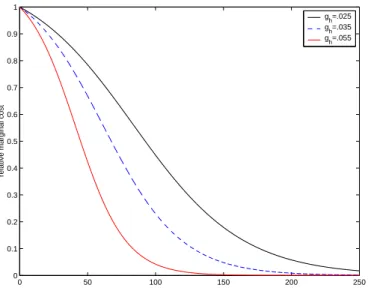
The loss of competitiveness follows the path illustrated in figure 2. Under policy rule (13), the distribution of market shares across goods of different age is time invariant. Therefore the two competitiveness-loss functions (one backward looking, ¯m/ms, the other
forward looking, ¯mτ/mt, in (16)) are independent of τ and coincide for s≡(t−τ).
14
That the tax per unit of emissions increases along balanced growth paths with declining pollution intensity of output is a result common to all models with emissions inputs. In fact, asP/Y declines, the marginal product of emissions increases, and this is reflected in their implicit price.
15
0 50 100 150 200 250 0
0.1 0.2 0.3 0.4 0.5 0.6 0.7 0.8 0.9 1
t
relative marginal cost
g
h=.025
gh=.035 g
h=.055
Figure 2: Competitiveness-loss or “green crowding-out” effect
3.1
The aggregate economy
We use three aggregation factors, Γ, Λ and ∆, to express aggregate variables as propor-tional to the corresponding variables in the leading-edge sector. In appendix A.1 we define these factors and present their properties.16 We can then compute aggregate demand for capital from the intermediate goods sector by integrating over the space of goods the rearranged production function (2), to obtain:
Kτ = ¯Aτx¯τΓ (17)
Similarly, using (1), (2) and (4) the flow of aggregate emissions and output is:
Pτ = Z
1
αβ
τ A¯τx¯τΛ (18)
Yτ = (1−n)1−αZτA¯τx¯ατ∆ (19)
It is worth spending a few words to explain the meaning of these aggregation factors. Consider ∆ that measures the relative contribution of older goods to production:
∆ =
Z 1
0
ZjτAjτxαjτ
ZτA¯τx¯ατ
dj =λn
Z ∞
0
e−(λn+g)s µ
¯
m
ms
¶1−αα
ds (20)
16
It is computed by taking into account the mass of existing goods of age s, their total productivity gap, and their relative use. Initially, each technology is embodied in a mass
λn of goods, out of which only a proportion e−λns of goods of age s survives at date τ.
Older goods are less productive than the leading-edge good, and their productivity gap is ruled by the growth rate of total productivity,AZ1/(1−α), which equalsg by (14). Finally, sales of older goods are affected by environmental policy according to the competitiveness-loss function ¯m/ms.
Substituting ¯xτ in (18) using (17), aggregate emissions are:
Pτ =Z
1
αβ τ Kτ
Λ
Γ (21)
which can be rearranged as follows :
Zτ =
µ PτΓ
KτΛ
¶αβ
(22)
Thus leading-edge pollution intensity also measures the pollution intensity of aggregate output. If ζ < 0 pollution intensity declines continuously for the economy as a whole, although the process is discontinuous at the firm level.
Next, substituting ¯xτ in (19) using (17), we obtain aggregate output as follows:17
Yτ =Zτ
£
(1−n) ¯Aτ
¤1−α
Kα
τ
∆
Γα (23)
Finally, substituting Z in (23) using (22), we can write emissions explicitly as inputs in the production function:
Yτ = ∆
£
(1−n) ¯Aτ
¤1−α "
µ Pτ
Λ
¶βµ
Kτ
Γ
¶1−β#α
(24)
It is clear then that the lower are emissions inputs the lower is output. Moreover, equation (24) shows that emissions are combined with services from capital goods, with unitary elasticity of substitution, and then this composite good is combined with labor.
To conclude on the aggregate picture of the economy, we find that green tax revenue
17
grows at the same rate as output. In fact, green tax revenue grows at rate gh+gP which
equals g from (21) under policy rule (13). Hence, transfers to households grow at this rate to keep the budget balanced. This property provides a simple implementation rule for policy (13): the tax level must be set so as to maintain constant the weight of green tax revenue over output.
3.2
General equilibrium
The dynamic general equilibrium is determined when the labor market clears and workers are indifferent as to whether they work in final sector firms or in R&D firms. The equi-librium level of R&D employment,n, equates labor productivity in the final sector (5) to the expected marginal return on R&D from the arbitrage condition (11), using (19):
(1−α) (1−n)−αZτA¯τx¯ατ∆ =λVτ
SubstitutingVτ using (16) and simplifying, the condition is:
(1−n)−αZτx¯ατ∆ = λ
α(r+H) ¯xτ
Z ∞
τ
e−(r+λn)(t−τ) µ
¯
mτ
mt−τ
¶1−αα
dt (E)
Figure 3 depicts the left-hand-side of equation (E) at a given date τ as an upward sloping, and the right-hand-side as a downward sloping schedule in the (n,value) space.18 The equilibrium level of R&D,ne, is determined at the intersection of the two schedules.
The left-hand-side is proportional to the marginal product of labor in the final sector. Due to diminishing returns, the latter decreases monotonically and tends to infinity as all labor is employed in R&D. The right-hand-side is proportional to the value of an innovation. The first factor before the integral, is proportional to the initial instantaneous profit of the innovator which is decreasing in n (see 16).19 Also the integral is strictly decreasing inn. This is straightforward for the discount factor and the survival probability. Furthermore, competitiveness loss proceeds at a faster pace, because the greater is the rate of innovation, the faster the green tax will be increasing, according to policy rule (13). The expected flow of profits is therefore crowded out at a faster rate.
It follows that, if atn = 0, the expected return to R&D is greater than the cost, there
18
Both the LHS and the RHS in figure 3 shift downwards over time. However they cross at a constant level ofn(see 25).
19
✲ ✻
LHS RHS
1
ne n
Figure 3: The equilibrium condition (E)
exists a unique equilibrium level of R&D activity, ne >0. Substituting ¯x
τ and ∆ in (E)
using (7) and (20), and simplifying, ne is defined as the implicit solution of:
n
α(1−n)
Z ∞
0
e−(g+λn)s µ
¯
m
ms
¶1−αα
ds =
Z ∞
0
e−(r+λn)t µ
¯
m mt
¶1−αα
dt (25)
4
The impact of environmental policy when the
di-rection of technological change is exogenous
Let us assume that the aggregate index of the direction of R&D, ζ, is exogenous, and in particular independent of environmental policy. Under policy rule (13) gh = −λnζ/αβ
always, and therefore the policy tool of interest is the level of the green tax burden levied on the leading-edge producer: H. In fact, at any given date Z is known, so that the policy-maker is able to set H = hZ1/αβ by controlling the tax h. In doing so it can actually set the burden of green tax levied on each vintage and can effectively manage the shape of the competitiveness-loss schedule. We find the following result.
Proposition 2 A marginal increase in the burden of the green tax levied on innovations,
H, increases the level of R&D employment on the balanced growth path if and only if innovations are environment-friendly. That is:
∂ne
∂H >0 iff ζ <0
Proof. See appendix A.2. The proof shows that, at the original equilibrium level of n, the left-hand-side of the equilibrium condition (E) falls more than its right-hand-side, ifζ <0.
These shifts of the schedules result in a new equilibrium with a highern.
A larger green tax burden directly reduces the innovator’s prospective profits and the value of innovations. The larger burden of taxation, however, also translates into a lower demand for labor from the final sector, which reduces the cost of R&D. The proposition establishes that the fall in wages outweighs the fall in the value of innovations, when these are environment-friendly. As a result R&D activity increases at equilibrium.
The asymmetric impact of the tax on the cost of and reward to R&D is due to the fact that an increase in the green tax weighs more heavily on older technologies than on more recent ones. In other words, market shares are skewed in favor of modern inter-mediate goods, because they are cleaner. It must be emphasized that in our framework environmental policy can foster R&D activity only if intermediate goods are differentiated in their pollution intensity and only to the extent that the tax affects the distribution of market shares across vintages.20 From this point of view, our result differs from those obtained in other multi-sector growth models, where environmental policy is favorable to the dynamic sector because it curbs demand for factors from the production sector (e.g. Verdier 1995, Elbasha and Roe 1996, Bretschger 1998, Hettich 1998).
Consider the reduced form of the equilibrium condition, (25). The downward shift of the competitiveness-loss schedule affects both sides of the equation. The left-hand-side represents the demand for labor from the final sector, which depends upon the distribution of sales across vintages. The reduction in the market share of relatively old goods is discounted according to their productivity gap, that is at rate g. The right-hand-side represents the demand for labor from the R&D sector, proportional to the value of an innovation. The latter depends upon the expected evolution of the market share of the patent holder. An expected fall in the future market share reduces the value of the patent according to discount rate r. Recall that along a balanced growth path r > g (the no-Ponzi games condition). Since the negative impact of an increase in the green tax burden falls more heavily on older sectors and on future profits, r > g implies that the loss has a heavier repercussion on labor demand from the final sector than from the R&D sector.
20
That∂n/∂H = 0 if ζ= 0 is established in the proposition. Furthermore,H affects the dynamics of the system only to the extent that it modifies the shape of the competitiveness-loss schedule. Suppose for instance that the marginal cost consists exclusively of the green tax burden, so that ¯m/mt=e−ght,
withgh exogenous in this setting. In this case the equilibrium R&D employment is independent ofH.
In other words, the current situation of the labor market depends less on expected future events than on past events, as summarized by the distribution of technologies embodied in the capital stock.
The main lesson we want to retain from this result is that environmental policies are in general not neutral with respect to the cross-sectorial distribution of demand. Green taxes skew sales towards cleaner intermediate goods. When there is a negative correlation between pollution intensity and technological age, the tax on emissions acts as a (relative) reward for most recent vintages. Therefore, if innovations are environment-friendly, environmental policy fosters innovative activities and leads to faster productivity growth (givenζ). The result can be interpreted along the lines proposed by Xepapadeas and de Zeeuw (1999).21 An increase in the green tax reduces the average age of capital goods in use, increasing the average productivity of capital. As in any endogenous growth model, higher return on capital fosters investment and increases the growth rate.
A complete study of the dynamics of the system is beyond the scope of this paper. Such an analysis requires solving functional differential equations of mixed type, since investment in R&D at any given point in time involves delays (productivity gaps and market shares of existing goods) and advances (expectations on competitiveness loss for innovations). As far as we know, recent mathematical results have been applied only to a few special cases in economics (Benhabib and Rustichini 1991). Among these studies, those that run numerical simulations find that on impact an unexpected permanent shock makes the control variable (investment) overshoot its new long term level (e.g. Boucekkine et al. 2004, Collard et al. 2004). These findings suggest that we can expect R&D employment to increase on impact as a result of an unexpected increase in H. This is a sufficient condition to establish that along a balanced growth path a marginal increase in
H, reduces on impact the level of aggregate output:22
∂Yτ
∂Hτ
<0
This is in fact true if R&D employment,nτ, does not decrease on impact. Moreover, the
recession is deeper the more environment-friendly are innovations, i.e. the lowerζ. Such a response from the economic system would not be surprising since we know from (24) that emissions are inputs in the aggregate production function. Thus the higher their relative price, the lower will be their employment and the lower the aggregate output for a
21
See Feichtinger et al. (2004) for a rigorous and thorough exploration of this argument.
22
given distribution of technologies embodied in the capital stock. This input effect is active even in the absence of differentiation in pollution intensity. However, with differentiation the impact is magnified because the policy change affects older (i.e. dirtier) goods more heavily. That is, for a given dH the average burden of green taxes is increasing in |ζ|.
5
The impact of environmental policy when the
di-rection of technological change is endogenous
In this section the model is extended to allow R&D laboratories to respond to tighter environmental policy by adopting cleaner technologies. Embodying cleaner technologies in blueprints, however, is costly for R&D firms. Pollution is a complementary input to capital for a given design, hence the use of lower emissions is, ceteris paribus, detrimental to a patent’s value. Consequently, R&D labs adopt cleaner technologies only if the incentives arising from environmental policy are strong enough. If this is the case then we can establish a correlation between environmental policy and the direction of technological change at the aggregate level: the tighter is environmental policy, the more environment-friendly are technologies. We explain this in the first and second parts of this section.
As is evident from (14), cleaner innovations (a larger |ζ|) reduce the expected contri-bution of any given amount of R&D to total productivity growth. This is nothing but the direct channel of transmission of environmental policy on growth, i.e. the dynamic version of the statement: “Given that pollution is an input, polluting less means produc-ing less”. This effect runs counter to the distortionary impact of environmental policy on market shares across vintages and thereby on R&D activity, described in the previous section. It follows that the comprehensive impact of tightening environmental policy on total productivity growth is ambiguous. By running simulations, however, we are able to show that, under the current specification of the model, growth is reduced by tighter environmental policy. The second and third parts of the section explore this argument.
5.1
Microeconomic background: the R&D lab’s choice of
pollu-tion intensity
Consider the problem of R&D firm i that has obtained an innovation in sector j, at date τ, with attached implicit labor productivity ¯Aτ. Suppose that it can choose to
with ¯Zτ =
R1
0 Zjτdj denoting the average pollution intensity in the economy at date τ.23 Note that the cross-sectorial spillovers concerning the two technological parameters are assumed to be similar in some respects. First and foremost, the set from which a successful R&D lab can choose the technology to adopt is determined entirely by spillovers from other sectors and is not sector specific.24 Second, while we assume that the leading-edge implicit labor productivity index characterizes innovations, we leave the choice of pollution intensity index up to the R&D lab. This is because this choice is not trivial and entails a trade-off, as illustrated below.
Let us denote by ˆZijτ ≤ Z¯τ the choice of the innovating R&D firm i in sector j. If
it employs ˆnijτ researchers it produces an expected instantaneous improvement in total
productivity equal toλnˆijτA¯τZˆ
1 1−α
ijτ . This is the correct measure of the (private) output of
an R&D firm. The lab could obtain the same expected instantaneous improvement in total productivity by employing less researchers, say ¯nijτ, if it were to adopt the most polluting
technology ¯Zτ instead of ˆZijτ. The mass of researchers ¯nijτ is given by λnˆijτA¯τZˆ
1 1−α ijτ =
λn¯ijτA¯τZ¯
1 1−α
τ . We can thus define the opportunity cost of targeting cleaner innovations
in terms of the percentage increase in research employment:
ˆ
nijτ
¯
nijτ
=
Ã
¯
Zτ
ˆ
Zijτ
!1−1α
≡ν³Z¯τ/Zˆijτ
´
We are now ready to formulate the problem of the R&D lab. It needs to decide the amount of “regular” researchers to be employed, ¯nijτ, and the degree of cleanliness of the
innovation it targets, ¯Zτ/Zˆijτ, taking as given all expected aggregate variables: {r, w, n}∞τ ,
23
It is fair to admit that imitation of the average technology is feasible. There is no concern on whether non-innovating firms adopt average pollution intensity. In fact, if the incumbent patent holder in sector
jwere to adopt the cleaner technology ¯Z, it would reduce the total productivity of its intermediate good. As a result it would face competition from previous, displaced producers in the sector. Only an innovator can adopt the clean technology, while keeping a safe margin over previous producers in terms of total productivity, thanks to its monopoly of technology ¯A (if (15) holds).
24
This crucial feature is necessary to keep the model tractable and for a balanced growth path to be feasible. In fact, only in this case the reward to R&D is independent of the sector, so that R&D activity is uniform across sectors, and the distribution of technological gaps across vintages is stationary on a balanced growth path.
hτ,gh, ¯Aτ, ¯Zτ. The choice is made in order to maximize the expected instantaneous return
on R&D employment, i.e.
max ¯
nijτ,Zˆijτ
λν³Z¯τ/Zˆijτ
´
¯
nijτVτ−ν
³
¯
Zτ/Zˆijτ
´
¯
nijτwτ
with Vτ =
Z ∞
τ
e−Rτtrsdse−λ
Rt τnsdsΠˆ
t( ¯Aτ,Zˆijτ)dt
The first order conditions of this problem give:
λVτ =wτ
which is a restatement of (11), and:25
∂Vτ
∂Zˆijτ
=
Z ∞
τ
e−Rτtrsdse−λ
Rt
τnsds
Ã
rt+hτZˆijτ1/αβ
rt+egh(t−τ)hτZˆijτ1/αβ
!1−αα "
egh(t−τ)h τZˆijτ1/αβ
rt+egh(t−τ)hτZˆijτ1/αβ
−β #
dt= 0
(26) Improving the cleanliness of the innovation affects its value in two opposite directions. On the one hand, profits accruing to the patent holder are reduced because the innovation’s total productivity, ¯AτZˆ
1 1−α
ijτ , falls. On the other hand, if emissions are taxed, profits
increase because the burden of the green tax on marginal cost, hτZˆ
1
αβ
ijτ, is reduced. This
gain is in fact increasing in the expected growth rate of the green tax,gh.
Condition (26) balances out the cost and benefit of lower pollution intensity in expected present value terms. Its solution is such that the net present value of marginal investment in cleanliness equals zero. The solution is:
- ˆZijτ = ¯Zτ if gh = 0 and hτ ≤ 1−ββrτZ¯τ−1/αβ;
- ˆZijτ <Z¯τ if gh >0 or hτ > 1−ββrτZ¯τ−1/αβ. 26
5.2
Macroeconomic implications
We now examine the relationship between the behavior of the representative R&D lab-oratory and the evolution of key macroeconomic variables and policy instruments. The
25
In fact, the condition isλν(.) ¯nijτ∂Vτ/∂Zˆijτ −ν(.) ¯nijτ[λVτ−wτ]1−α1 /Zˆijτ = 0, where the second
term equals zero according to the other first order condition.
26
Notice that for ¯Z constant (i.e. when initially ˆZ = ¯Z), gh >0 implies that hτ > 1−ββ rτZ¯ −1/αβ τ at
analysis is restricted to balanced growth paths. First consider the macroeconomic vari-able determining the direction of technological change, i.e. parameterζ. Clearly when the representative firm chooses to adopt average pollution intensity - i.e. the most polluting technology in the menu - the distribution of pollution intensity indexes across vintages will converge to a uniform distribution, with all sectors sharing the same pollution intensity. This is the case when ζ = 0.
Let us define the leading edge pollution intensity as the one targeted by R&D lab-oratories, i.e. Zτ ≡ Zˆτ. Then we can compute the average pollution intensity along a
balanced growth path , as:
¯
Zτ =
Z 1
0
Zjτdj =λn
Z ∞
0
e−λnsZτ−sds=Zτ 1
1 +ζ
where we switch the space of integration as in appendix A.1. It follows that
ζ = 1− Zˆ¯τ
Zτ
(27)
leading to:
- ζ = 0 ifgh = 0 and hτ ≤ 1−ββrτZ¯τ−1/αβ;
- ζ <0 if gh >0 or hτ > 1−ββrτZ¯τ−1/αβ;
- ∂|ζ|/∂gh >0.27
It is also to be noticed that the instruments of environmental policy are now different from those of the previous section. In that case the direction of technological change was fixed, so that the growth rate of the green tax, gh, was set according to rule (13). As
a consequence the policy-maker had some degree of freedom only in setting the level of tax, hτ, and thus the burden of the green tax levied on innovations, H. Instead when
innovators choose the pollution intensity of their blueprints, the environmental policy-maker loses control over the burden of the green tax levied on these agents, H. In fact when ˆZτ <Z¯τ, a once and for all upward jump in the green tax, hτ, entails a symmetric
27
adjustment of the pollution intensity target, according to28
dZˆτ
dhτ
hτ
ˆ
Zτ
=−αβ
Given ˆZτ ≡ Zτ, this response is such that Hτ = hτZ1τ/αβ is independent of hτ. In this
case, therefore, the policy tool upon which the policy-maker has some leverage isgh. We
assume that a credible commitment on the growth rate of the green tax is possible. This seems plausible because it only requires that the government keep constant the share of green tax revenue over GDP. As we have argued, expectations over gh do determine the
direction of technological change. Hence, by allowing gh to be set freely policy rule (13)
still holds, although causality is now reversed.
We can now ask how the balanced growth path of the economic system is affected by a stricter environmental policy. A commitment to a highergh augments the incentive
to adopt cleaner technologies, a choice that lowers the total productivity of innovations. This translates directly into a slower productivity growth. It can be seen from (14) that, holding n constant, g falls as |ζ| increases. This is the direct channel of transmission of environmental policy on growth. Nevertheless, whengh >0 innovations are
environment-friendly and pollution intensity is heterogeneous across goods. As a result, tightening environmental policy permanently modifies the distribution of market shares across vin-tages and, through this indirect effect, affects the equilibrium level of R&D employment,
n. The rise in gh affects this distribution in two ways: the relative weight of the initial
tax burden (H/r) changes, and the tax burden increases at a faster pace with age. The competitiveness loss schedule shifts downwards and favors innovations. The expected implication of this structural change is to foster R&D activity, i.e. to increase n. Un-fortunately, however, this last indirect effect cannot be determined exactly. To establish how n responds to gh it is necessary to solve the dynamic equilibrium, since R&D is a
form of investment that reacts to technological opportunities according to preference pa-rameters, such as the willingness to smooth consumption. Moreover, even when a higher
gh does foster R&D activity, the global impact of stricter environmental policy on growth
is ambiguous. In fact, even if more researchers were employed, the expected contribution of each of them to productivity growth is reduced by the direct channel of transmission.
28
5.3
Numerical simulations
In the case of an endogenous direction of R&D we solve numerically the system given by the equilibrium condition (25), the first order condition (26) and the policy rule (13). So-lutions in terms of{n, Zτ, ζ}are derived for balanced growth paths prevailing for different policies gh. Figure 4 plots the results obtained for the baseline case.29 The simulations
confirm that the direct channel of transmission of environmental policy on growth dom-inates the indirect effect. The growth rate declines monotonically with gh. However, a
faster growth of green taxes stimulates R&D activity, a secondary effect that eases the slowdown in productivity growth. The cost of environmental policy in terms of slower growth is reduced by its positive impact on incentives to engage in R&D activity. More-over, the adoption of cleaner technologies improves the efficiency of environmental policy in targeting any given goal in terms of rate of growth of polluting emissions.
0 0.1 0.2
0.22 0.24 0.26
g
h
R&D employment
0 0.1 0.2
−0.3 −0.2 −0.1 0
g
h
growth of output and emissions
g g
h
0 0.1 0.2
0.15 0.2 0.25 0.3 0.35
g
h
wage
0 0.1 0.2
0 0.05 0.1
g
h
value of innovations
0 0.1 0.2
−0.1 −0.05
0
gh direction of R&D
0 0.1 0.2
0.8 0.85 0.9 0.95 1
gh initial pollution intensity
Figure 4: Endogenous direction of R&D: equilibria as function ofgh.
29
The values of parameters are set atα=.4,β =.125,λ=.5,γ=.2,A0= 1,hτ =.02,ρ=.03, and
ε= 1.5. We concentrate on the presentation of the baseline case because changing the parameters (but
In order to asses the importance of the distortionary impact of environmental policy in easing the growth-environment trade-off, we compare the results with those obtained from a benchmark model based on Grimaud and Ricci (1999). In the benchmark model intermediate goods are not differentiated in pollution intensity, so that intermediate-goods producers chooseZ at each date to maximize their instantaneous profits. Pollution intensity is in effect a control variable, rather than a state variable, in the benchmark model. Figure 5 compares the results concerning R&D employment and growth rate, for the case with ε = .9. This case is particulary interesting because the substitution effect dominates the income effect, so that households invest less when the rate of return on savings falls. Since R&D is a form of investment, the standard result is that stricter environmental policy is detrimental to R&D activity. In our case instead the distortionary impact of green taxes is strong enough to reverse the standard outcome.
0 0.1 0.2
0.25 0.255
gh R&D employment levels
0 0.1 0.2
0 0.01 0.02
gh growth rates
0 0.1 0.2
0 0.005 0.01 0.015 0.02 0.025
g
h
% difference in n
0 0.1 0.2
0 0.005 0.01 0.015 0.02 0.025
g
h
% difference in g
Figure 5: The distortionary impact of green taxes: comparison of models with (-) and without (- -) differentiation in pollution intensity.
for our unambiguous numerical result is the strong response of R&D labs in adopting much cleaner technologies when environmental policy is tightened. In turn, this is the consequence of two assumptions. First, differently from Hart (2004 a), R&D labs face an almost unconstrained technology menu ˆZ ∈ (0,Z¯]. Second, production technology is characterized by unitary elasticity of substitution for emissions with capital and effective labor. However, recent findings suggest that dynamic multi-sector models depend crucially on the assumed degree of elasticity of substitution (e.g. Bretschger and Smulders 2004). Thus an applied version of our theory should go beyond these assumptions.
6
Conclusion
In the theory presented in this paper, economic growth results from the design of new, more productive capital goods by profit seeking agents, the R&D firms. Emissions rep-resent implicit inputs complementary to capital. Hence, if new goods are designed as cleaner, their productivity is below their potential level. If the tax on emissions is large enough, innovations are relatively clean. This has two implications. First, the contri-bution of innovation to growth in productivity is weakened. Second, capital goods are differentiated in pollution intensity. The latter effect gives scope for taxation to distort the distribution of market shares across goods of different vintages. In particular, the green tax increases the market share of relatively modern goods (which are the most pro-ductive and the least polluting), and this effect improves incentives to engage in R&D activities. The crucial assumption underlying this result is that R&D is labor intensive.30 The identification and exploration of this second channel of transmission of environmental policy constitutes the main original contribution of the paper.
To summarize, a restrictive environmental policy affects economic growth through two channels of transmission that operate in two opposite directions: the first channel lowers the marginal impact of innovation on productivity growth, while the second channel spurs innovation. The second channel is unlikely to dominate unless R&D labs have little scope for reducing pollution intensity. In any case, when carrying out cost-benefit analyses of environmental policy, its cost in terms of slower growth is reduced once this distortionary impact of policy on competition across vintages is taken into account.
Finally, we would like to point out that the distortionary impact of green taxes high-lights a more general property of the Schumpeterian model of growth. In fact, in the
30
multi-sector model of vertical innovation where labor is the sole input in R&D, any policy that affects heterogeneously the producers of intermediate goods has an impact on the equilibrium growth of output (Ricci 2002). Various policies influence the distribution of market shares across goods of different vintages, for instance tax breaks for new firms or fiscal incentives to adopt new equipment. This additional property confirms the fact that the Schumpeterian theory of growth is a fruitful tool for policy analysis.
References
Aghion, P. and P. Howitt (1992), ‘A Model of Growth Through Creative Destruction’.
Econometrica 60(2), 323-351.
Aghion, P. and P. Howitt (1998)Endogenous Growth Theory. First ed. Cambridge: The MIT Press.
Andreoni, J and A. Levinson (2001), ‘The Simple Analytics of the Environmental Kuznets Curve’. Journal of Public Economics 80(2), 269-286.
Benhabib, J. and A. Rustichini (1991), ‘Vintage Capital, Investment and Growth’. Jour-nal of Economic Theory 55: 323-339.
Bretschger, L. (1998), ‘How to Substitute in order to Sustain: Knowledge Driven Growth under Environmental Restrictions’. Environmental and Development Economics 3: 425-442.
Bretschger, L. and S. Smulders (2004), ‘Sustainability and Substitution of Exhaustible Natural Resources. How Resource Prices Affect Long-Term R&D Investment’. WIF-Institute of Economic Research, Economics w.p. 03/26, ETH Zurich.
Bovenberg, A.L. and S. Smulders (1995), ‘Environmental Quality and Pollution-Augmenting Technological Change in a Two-Sector Endogenous Growth Model’. Journal of Public Economics 57(3): 369-391.
Boucekkine, R., O. Licandro, L.A. Puch and F. del Rio (2004), ‘Vintage Capital and the Dynamics of the AK Model’. Journal of Economic Theory, forthcoming.
Collard, F., O. Licandro and L.A. Puch (2004), ‘The Short-run Dynamics of Optimal Growth Models with Delays’. Mimeo, European University Institute, Florence.
Elbasha, E. and T. Roe (1996), ‘On Endogenous Growth: The Implications of Envi-ronmental Externalities’. Journal of Environmental Economics and Management 31: 240-268.
Feichtinger, G., R. Hartl, P. Kort and V. Veliov (2004), ‘Environmental Policy, the Porter Hypothesis and Composition of Capital: Effects of Learning and Technological Progress’.
Journal of Environmental Economics and Management, forthcoming.
Gradus, R. and S. Smulders (1993), ‘The Trade-Off Between Environmental Care and Long-Term Growth–Pollution in Three Prototype Growth Models’. Journal of Economics 58(1): 25-51.
Grimaud, A. (1999), ‘Pollution Permits and Sustainable Growth in a Schumpeterian Model’. Journal of Environmental Economics and Management 38(3): 249-266.
Grimaud, A. and F. Ricci (1999), ‘The Growth-Environment Trade-off: Horizontal vs Vertical Innovations’. Fondazione ENI E. Mattei w.p. 99.34, Milan.
Grossman, G. and E. Helpman (1991),‘ Quality Ladders in the Theory of Growth’. Review of Economic Studies 58(1): 43-61.
Hettich, F. (1998), ‘Growth Effects of a Revenue-Neutral Environmental Tax Reform’.
Journal of Economics 67(3): 287-316.
Hettige, H., M. Mani and D. Wheeler (1998), ‘Industrial Pollution in Economic Develop-ment (Kuznets Revisited)’. World Bank, Policy Research w.p. 1876, Washington.
Hart, R. (2004 a), ‘Growth, Environment and Innovation: A Model with Production Vintages and Environmentally Oriented Research’. Journal of Environmental Economics and Management 48(3): 1078-1098.
Hart, R. (2004 b), ‘Can Environmental Policy Boost Growth?’. Paper presented at the Monte Verit`a Conference on Sustainable Resource Use and Economic Dynamics, Ascona (Switzerland), June 7-10. Organized by the Institute of Economic Research of ETH Zurich.
Jaffe, A., R. Newell and R. Stavins (2002), ‘Environmental Policy and Technological Change’. Envionmental and Resource Economics 22(1-2): 41-69.
Michel, P. (1993), ‘Pollution and Growth Towards the Ecological Paradise’. Fondazione ENI E. Mattei w.p. 80.93, Milan.
Michel, P. and G. Rotillon (1995), ‘Disutility of Pollution and Endogenous Growth’.
Environmental and Resource Economics 6(3): 279-300.
Mohtadi, H. (1996), ‘Environment, Growth, and Optimal Policy Design’. Journal of Public Economics 63(1): 119-140.
Popp, D. (2002), ‘Induced Innovation and Energy Prices’. American Economic Review 92: 160-180.
Ricci, F. (2000), ‘Essays on the Theory of Sustainable Development’. Ph.D. dissertation, Universit´e de Toulouse 1.
Ricci, F. (2002), ‘The Growth Effect of Cross-Sectoral Distortions’. Temi di Ricerca dell’Ente “Luigi Einaudi” w.p. no.26, Rome.
Ricci, F. (2004), ‘Channels of Transmission of Environmental Policy to Economic Growth: A Survey of the Theory’. Fondazione ENI E. Mattei w.p. 52-04.
Stokey, N. (1998), ‘Are there Limits to Growth ?’. International Economic Review 39(1): 1-31.
van Marrewijk, C., F. van der Ploeg and J. Verbeek (1993), ‘Is Growth Bad for the Environment? Pollution, Abatement and Endogenous Growth’. World Bank, Policy Research (Environment) w.p. 1151, Washington.
Van Zon, A. and H. Yetkiner (2003), ‘An Endogenous Growth Model with Embodied Energy-Saving Technical Change’. Resource and Energy Economics 25: 81-103.
Verdier, T. (1995), ‘Environmental Pollution and Endogenous Growth: a Comparison between Emission taxes and Technological Standards’, in C. Carraro and J.A. Filar, ed.s,
Control and Game-Theoretic Models of the Environment (Annals of the International Society of Dynamic Games). Boston, Basel and Berlin: Birkhauser. Vol.2: 175-200.
Xepapadeas, A. (1994), ‘Long-Run Growth, Environmental Pollution, and Increasing Re-turns’. Fondazione ENI E. Mattei w.p. 67.94, Milan.
Xepapadeas, A. and A. de Zeeuw (1999), ‘Environmental Policy and Competitiveness: The Porter Hypothesis and the Composition of Capital’. Journal of Environmental Eco-nomics and Management 37(2): 165-182.
A
Appendix
A.1
The aggregation factors
Γ
,
Λ
and
∆
We compute sales of goodj relative to the leading-edge sector, using (7), as:
ˆ xjτ
¯ xτ
=
µ
Zjτ
Zτ
¶1−α1 µ
¯ m mj
¶1−α1
By definition (see (2) and (17)):
Γ =
Z 1
0 Ajτ
¯ Aτ
ˆ xjτ
¯ xτ
dj
The integral has no mathematical sense because Ajτ
¯
Aτ and Zjτ
Zτ are distributed stochastically (and
a priori discontinuously) over the space of goods [0,1]. However at any date τ we can reshuffle goods according to their technological gap, i.e. their ages. Along a balanced growth path each technology is initially adopted by λn of firms, out of which only a proportion e−λns of those ageds survives at date τ. The productivity gap for firms of age s is: A¯τ−s
¯
Aτ =e
−gA¯s
=e−λnγs; and the pollution intensity gap is: Zτ
Zτ−s =e
less, according to the competitiveness-loss function, ¯m/ms. Using (14) we have:
Γ =
Z ∞
0
λne−λnsA¯τ¯−s Aτ
µ
Zτ−s Zτ
¶1−α1 µ
¯ m ms
¶1−α1
ds
= λn
Z ∞
0
e−(λn+g)s
µ
¯ m ms
¶1−α1
ds
By definition (see (4), (17) and (18)) and proceeding as above:
Λ = Z 1 0 µ Zjτ Zτ
¶αβ1
Ajτ ¯ Aτ ˆ xjτ ¯ xτ dj = λn Z ∞ 0 e− ³
λn+g+αβζ λn´sµ m¯
ms ¶1−1α
ds (28)
By definition (see (1) and (19)) and using (14):
∆ = Z 1 0 Zjτ Zτ Ajτ ¯ Aτ µ ˆ xjτ ¯ xτ ¶α dj = λn Z ∞ 0
e−(λn+λnγ+λnζ)s
µ
Zτ−s Zτ
¶1−αα µ
¯ m ms
¶1−αα
ds
= λn
Z ∞
0
e−(λn+g)s
µ
¯ m ms
¶1−αα
ds
We have the following properties :
Property 1 : Γ<1, ifζ <0, from (13), (14) and (15).
Property 2 : Λ>Γ if ζ <0sincezj−1/αβ∈[1,∞).
Property 3 : Λ>∆>Γ, if ζ <0. Indeed using (13) :
∆ = Z 1 0 Ajτ ¯ Aτ µ Zjτ Zτ
¶1−1αµm¯
mj ¶1−αα
dj = Z 1 0 Ajτ ¯ Aτ µ Zjτ Zτ ¶ 1 1−αµm¯
mj ¶
1
1−α r+H
³ Zjτ
Zτ
´αβ1
r+H dj
= r
r+HΓ + H r+HΛ
Thus : ∆−Λ = r+rH(Γ−Λ)<0, by property 2.
Define G=γ+ζ/(1−α). By Jensen’s inequality:
[∆(1 +G)]α1 =
(
λn
Z ∞
0
(1 +G)e−(1+G)λns
" µ
¯ m ms
¶1−1α
#α ds ) 1 α ≤ ≤ λn Z ∞ 0
(1 +G)e−(1+G)λns
µ
¯ m ms
¶1−1α
ds= Γ(1 +G)
Property 5 : Γ = ∆ = Λ =R1
0
Ajτ
¯
Aτ dj = (1 +γ)
−1 ifζ = 0
If there is no differentiation in pollution intensity, that is ifζ = 0, thenZjτ/Zτ= 1∀j∈[0,1],
andgh = 0 by policy rule (13), so that ˆxjτ/x¯τ = 1 ∀j∈[0,1], which proves the result.
A.2
Proof of proposition 2
To prove the result we show that, at the original equilibrium level ofn, the left-hand-side (LHS) of the equilibrium condition (E) falls more than the right-hand-side (RHS). These shifts of the schedules depicted in figure 4.b result in a higher equilibrium level of R&D employment,n.
Preliminary: The LHS of (E) can also be written as Yτ/ £
(1−n) ¯Aτ ¤
and therefore falls along with output. Let us first differentiate output given by (19) with respect toH≡hZ1/αβ, holding n constant. Using (7), (20), (28), definitions in appendix A.1 and property 3, we have:
∂Y ∂H ¯ ¯ ¯ ¯ dn=0
= (1−n)1−αZτA¯τx¯ατ · ∂∆ ∂H + α∆ ¯ xτ
∂x¯τ
∂H
¸
= α(1−n) 1−αZ
τA¯τx¯ατ
(1−α) [r+H]
" Z 1 0 Zjτ Zτ Ajτ ¯ Aτ µ ˆ xjτ ¯ xτ
¶α"
1−
µ
Zjτ
Zτ
¶αβ1 #
r mj
dj−∆
#
= A¯τx¯τ α(1−α)
" r ¯ m Z 1 0 Ajτ ¯ Aτ ˆ xjτ ¯ xτ
dj− r
¯ m Z 1 0 Ajτ ¯ Aτ ˆ xjτ ¯ xτ µ Zjτ Zτ
¶αβ1
dj−∆
#
= A¯τx¯τ α(1−α)
hr
¯ mΓ−
r ¯ mΛ−∆
i
= A¯τx¯τ α(1−α)
·
∆−H
¯ mΛ−
r ¯
mΛ−∆
¸
= −A¯τx¯τ
α(1−α)Λ<0 (29)
Remark: ¯ ¯∂Y∂H
¯ ¯
dn=0
¯
¯ is increasing in|ζ|. In factζ = 0 ⇒∂∆/∂H = 0 by property 5 in appendix
A.1,⇒ R01 Zjτ Zτ Ajτ ¯ Aτ ³ ˆ xjτ ¯ xτ
´α·
1−³Zjτ Zτ
´αβ1 ¸
r
mjdj= 0. Instead ζ <0 ⇒
³
Zjτ Zτ
´αβ1
>1 ∀j but one,
⇒R01 Zjτ Zτ
Ajτ
¯
Aτ
³xˆ
jτ
¯
xτ
´α·
1−³Zjτ Zτ ´ 1 αβ ¸ r
mjdj<0.
Using (29) inLHS ≡Yτ/£(1−n) ¯Aτ¤we obtain:
∂LHS ∂H =
−x¯τΛ