Submitted20 March 2014 Accepted 18 April 2014 Published8 May 2014 Corresponding author
Ping Ding, [email protected]
Academic editor
Stuart Pimm
Additional Information and Declarations can be found on page 10
DOI10.7717/peerj.374 Copyright
2014 Si et al.
Distributed under
Creative Commons CC-BY 4.0 OPEN ACCESS
How long is enough to detect terrestrial
animals? Estimating the minimum
trapping e
ff
ort on camera traps
Xingfeng Si1, Roland Kays2and Ping Ding1
1The Key Laboratory of Conservation Biology for Endangered Wildlife of the Ministry of Education, College of Life Sciences, Zhejiang University, Hangzhou, Zhejiang, China 2North Carolina Museum of Natural Sciences & NC State University, Raleigh, NC, USA
ABSTRACT
Camera traps is an important wildlife inventory tool for estimating species diversity at a site. Knowing what minimum trapping effort is needed to detect target species is also important to designing efficient studies, considering both the number of camera locations, and survey length. Here, we take advantage of a two-year camera trapping dataset from a small (24-ha) study plot in Gutianshan National Nature Reserve, eastern China to estimate the minimum trapping effort actually needed to sample the wildlife community. We also evaluated the relative value of adding new camera sites or running cameras for a longer period at one site. The full dataset includes 1727 independent photographs captured during 13,824 camera days, documenting 10 resident terrestrial species of birds and mammals. Our rarefaction analysis shows that a minimum of 931 camera days would be needed to detect the resident species sufficiently in the plot, andc. 8700 camera days to detect all 10 resident species. In terms of detecting a diversity of species, the optimal sampling period for one camera site wasc. 40, or long enough to record about 20 independent photographs. Our analysis of evaluating the increasing number of additional camera sites shows that rotating cameras to new sites would be more efficient for measuring species richness than leaving cameras at fewer sites for a longer period.
Subjects Biodiversity, Conservation Biology, Ecology, Zoology
Keywords Animal inventory, Species richness, Gutianshan, Wildlife monitoring, Species accumulation curves, Sampling effort, Camera day
INTRODUCTION
new surveys are designed without guidance or following untested rules of thumb about the sampling effort needed to reach their goals.
One key metric that is useful for planning efficient studies documenting diversity of wildlife in a particular area is the minimum trapping effort (MTE). MTE is the trapping effort–the number of camera days–required to record the species of interest in a specific area (Yasuda, 2004). Estimates of MTE allow the design of an efficient inventorying plan that does not extend too long, nor fail to detect some species present in the survey area. The trapping efforts reported in the literature varies widely (Maffei, Cu´ellar & Noss, 2004;
Wegge, Pokheral & Jnawali, 2004;Trolle & K´ery, 2005;Li et al., 2010). Even for the same species, the MTE varies widely across studies, for example, the recommended trapping efforts varied from 450 camera days in Bolivia (Trolle & K´ery, 2003) to 2280 in Brazil (Maffei et al., 2005) for targeting the ocelot (Leopardus pardalis). Factors that might affect the MTE include habitat, weather conditions, abundance of target species, and sampling strategies such as the use of baits and spacing of cameras (Wegge, Pokheral & Jnawali, 2004;Rovero & Marshall, 2009). Furthermore, a variety of different statistics have been used to estimate MTE, including species accumulation curves (Wegge, Pokheral & Jnawali, 2004;Azlan, 2006), calculations based on the probability of capture (Tobler et al., 2008), simulation models (Rowcliffe et al., 2008), sampling precision analysis (Rovero & Marshall, 2009) and bootstrap procedures based on the precision of parameter estimation (Goswami et al., 2012). Finally, there is little distinction between the number of camera days and the number of camera sites, in these studies.
Similar to the MTE in studies of camera traps, the minimal area of a plant community is a classic concept introduced in the 1920s (Hopkins, 1957), and regularly discussed since then (Goodall, 1952;Hopkins, 1957;Whittaker, 1980;Barkman, 1989). The related curve, known as the species accumulation curve, is the relationship of the number of species and the sampling effort, which may depend on the time or area sampled. One expects curves to approach an asymptote, and thus give a judgment of sampling adequacy (Daubenmire, 1968). In long-term monitoring projects, sampling over gradients in time is logically similar to sampling over gradients in space (Colwell & Coddington, 1994). Thus, for camera traps, the relationship between trapping efforts and the number of species detected is analogous to the minimal area concept (Adler et al., 2005). With increasing trapping efforts, the species richness should level offwhen the sampling effort (i.e., camera days) is large enough, meaning the inventorying of wildlife species is sufficient. If we know the total species diversity in the area, we then can assess trapping efforts on the species-trapping effort relationship to a certain probability of total species.
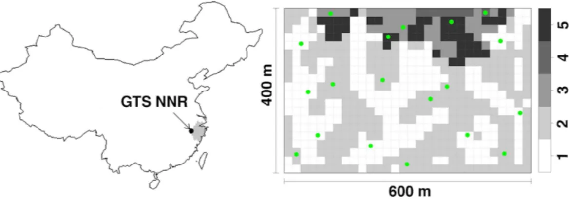
Figure 1 The research site.The location of research plot in Gutianshan National Nature Reserve (GTS NNR) in western Zhejiang Province (grey portion), eastern China, and 19 camera sites (green dots) randomly stratified across habitat types (valleys, ridges, mid-slopes, high slopes and high ridges as numbered from 1 to 5, respectively) in the research plot.
number of terrestrial species added as trapping effort increases, and then evaluate the MTE based on a certain probability of total species. We also evaluate the relative value of adding new camera sites or running cameras for a longer period at one site, and assess the optimal sample period for efficient species detection per camera site.
MATERIALS & METHODS
Ethics statementOur research on camera traps in Gutianshan National Nature Reserve was approved by the Chinese Wildlife Management Authority and conducted under Law of the People’s Republic of China on the Protection of Wildlife (August 28, 2004).
Field site
We deployed camera traps in a permanent plot (400 m×600 m), which is located in the old-growth forest of the Gutianshan National Nature Reserve (hereafter, the Reserve) (Fig. 1; 29◦15′6′′–29◦15′21′′N, 118◦7′1′′–118◦7′24′′E) (Liu et al., 2012). The protected area
of the Reserve is approximately 81 km2, with 57% as natural forest. The Reserve was set up to protect a portion of the old-growth evergreen broad-leaved forest.Castanopsis eyreiand
Schima superbaare the dominant species in this forest and in the plot. Most of the forest in our plot is now in the middle and late successional stages (Legendre et al., 2009). The annual mean temperature in this region is 15.3◦
C and annual mean precipitation is 1964 mm according to the data from 1958 to 1986 (Yu et al., 2001). The vegetation is dense and thick with ac. 12-m high canopy layer, a rather closed,c. 5-m high understory and a densec. 1.8-m high shrub layer (Chen et al., 2009). The elevation of our study plot ranges from 446 to 715 m and includes five habitat types in terms of topographic variations: valleys, ridges, mid-slopes, high slopes, and high ridges (Legendre et al., 2009).
Camera positioning
April 20, 2009 to September 14, 2011 (Fig. 1). The plot was divided into 600 20 m×20 m subplots.Legendre et al. (2009)classified these subplots into five habitat types in terms of topographic variations: valleys (237 subplots), ridges (269), mid-slopes (41), high slopes (8) and high ridges (45) as numbered from 1 to 5 inFig. 1. Based on the number of subplots of each habitat type, we randomly selected seven, seven, two, one, and two camera sites (all 19 sites) for each habitat type, respectively. We chose the specific positions of camera sites to optimize viewing angle from the tree on which they were mounted. We locked cameras to trees at heights of 40–50 cm above the ground. Cameras faced north or south to reduce the influence of false trigger by the sunrise and sunset. We removed branches or grasses immediately in front of cameras to avoid vegetation from triggering the cameras. A waterproof cover above the camera reduced the effects of rain on our electronics. We did not target animal trails where animal activity is concentrated, and did not use bait or lure to ensure that we only observed the natural movements of animals (Long et al., 2008;Rowcliffe et al., 2011). We set cameras to take one photograph after each trigger with the interval time of one second. We set all cameras to work 24 h a day and checked memory cards and batteries every month.
Statistical analysis
Our analyses focus on 19 camera sites with two years of continuous data from June 1, 2009 until May 31, 2011 (730 total days). We excluded seven arboreal birds and squirrels from the analyses (Tobler et al., 2008). We also exclude two pheasants (detected one and three times, respectively) and one mammal (detected seven times) in two years, considering these to be nonresident animals passing through the plot from their specialized habitats known to exist in other parts of the Reserve (Dong, 1990;Zhuge, 1990). We conducted all analyses in R (R Development Core Team, 2010).
Individuals of some species will trigger the camera multiple times in a row as they slowly forage at a camera site, resulting in dozens of photographs of the same individual (Kauffman et al., 2007). To exclude this influence of replicated photographs triggered by one individual, we set the interval time of 30 min to segregate independent detections of the same species (Otis et al., 1978;O’Brien, Kinnaird & Wibisono, 2003;Li et al., 2010). We used the R functionspecaccuminveganlibrary to conduct our rarefaction analysis (Oksanen et al., 2013). The sampling unit in our analyses is one monitoring day. Because we had 19 cameras working simultaneously in the plot, one monitoring day represents 19 camera days (one camera monitoring one day). We then used the rarefaction method to produce the species-trapping effort relationship.
Rarefaction analysis calculates the expected number of species in a small sample of individuals drawn at random from a census or collection (Simberloff, 1978;James & Rathbun, 1981), and allows for meaningful standardization and comparison of datasets with difference sampling efforts (Colwell, 2013;Gotelli & Colwell, 2001). So, the rarefaction curve represents a relationship between the number of species(S)and the camera days(D):
We defined the value ofps as the proportion of common resident terrestrial species (defined common resident species as P2 inTable 1>1%) in a collection such that
ps=S/Smax (2)
whereSmaxis the total number of species. We used the R functionspecpoolinvegan library (Oksanen et al., 2013) through the Chao’s method (Chao, 1987) to estimate the number of unseen species along with the observed species richness (Colwell & Coddington, 1994;Gotelli & Graves, 1996).Smaxwas calculated by extrapolating species richness in a species pool:
Smax=Sobs+a21/(2a2) (3)
whichSobsthe observed species richness,a1anda2are the number of species occurring
only in one or only in two sites in the collection. Then we usedEq. (1)to replaceSin
Eq. (2), and rearranged the formation ofEq. (2)as the proportion of species detected to the number of species richness:
f(D)=ps×Smax. (4)
With the criteria ofps, we carried out trapping efforts from the rarefaction curve.
We conducted a separate analysis to compare the relative value of adding sample days or new sample sites. For each trapping effort (camera days), for example, 10 camera sites monitoring 50 days separately, we sampled 10 camera sites of 19 and continuously sampled 50 days of 730. We calculated the proportion of species in the sampled data. We resampled 1000 times for each trapping effort and obtained the mean value of proportion of species to construct a contour map.
To evaluate how long a camera should be run at one site before cameras should be rotated, we estimated the average values of species richness for each camera site using rarefaction analyses against increasing of monitoring days and independent photographs, respectively.
RESULTS
Basic field results
Table 1 Summary of detected species during two years of camera trap monitoring in Gutianshan research plot.
Order/Family English name Latin name RP* IP* P1* P2*
GALLIFORMES
Phasianidae Chinese bamboo partridge Bambusicola thoracicus 3 3 0.17
Silver pheasant Lophura nycthemera 290 158 8.85 9.15
Elliot’s pheasant Syrmaticus ellioti 48 37 2.07 2.14
Koklass pheasant Pucrasia macrolopha 1 1 0.06
PICIFORMES
Picidae Grey-headed woodpecker Picus canus 8 5 0.28
PASSERIFORMES
Pittidae Fairy pitta Pitta nympha 1 1 0.06
Turdidae Golden mountain thrush Zoothera dauma 16 15 0.84
White-browed thrush Turdus obscurus 1 1 0.06
Pale thrush Turdus pallidus 4 4 0.22
Timaliidae Great necklaced laughingthrush Garrulax pectoralis 3 3 0.17 RODENTIA
Muridae Confucian niviventer Niviventer confucianus 1099 826 46.25 47.83 Edwards’s long-tailed giant rat Leopoldamys edwardsi 59 30 1.68 1.74 Sciuridae Pallas’s squirrel Callosciurus erythraeus 30 19 1.06 CARNIVORA
Viverridae Masked palm civet Paguma larvata 95 89 4.98 5.15
Mustelidae Hog badger Arctonyx collaris 81 36 2.02 2.08
Small-toothed ferret-badger Melogale moschata 8 7 0.39 0.41
Eurasian badger Meles meles 11 7 0.39
ARTIODACTYLA
Suidae Wild boar Sus scrofa 196 34 1.9 1.97
Cervidae Reeves muntjac Muntiacus reevesi 643 242 13.55 14.01
Black muntjac Muntiacus crinifrons 709 268 15.01 15.52
Notes.
*RP, recorded photographs(n); IP, independent photographs(n); P1, proportion of independent photographs (%), and
P2, proportion of independent photographs without the arboreal and transient animals (%).
grey-headed woodpecker (Picus canus: five photographs), fairy pitta (Pitta nympha: one), golden mountain thrush (Zoothera dauma: 15), white-browed thrush (Turdus obscurus: one), pale thrush (Turdus pallidus: four), great necklaced laughingthrush (Garrulax pectoralis: three), and Pallas’s squirrel (Callosciurus erythraeus: 19). Three species whose habitats are beyond the plot were also excluded: Chinese bamboo partridge (Bambusicola thoracicus: three), koklass pheasant (Pucrasia macrolopha: one), and Eurasian badger (Meles meles: seven all in one month).
Minimum trapping effort
In our plot, there were nine common resident species in 10 (Table 1). Therefore, we set
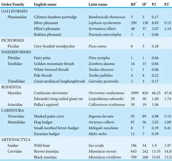
Figure 2 The species-trapping effort relationship for the communities of the terrestrial animals.We used rarefaction analysis to generate the species-trapping effort relationship. The 10 resident terrestrial species were detected during 13,824 camera days (seeTable 1). Because 19 cameras in our study were working simultaneously in the field, each monitoring day represents 19 camera days. The dashed lines indicate the 95% estimated confidence intervals. The inner graph is an enlargement of the first 150 monitoring days, showing how this relationship increased.
(931 camera days) of the MTE to trap all common resident species efficiently, andc. 8700 camera days to trap all 10 residents (Fig. 2).
The proportion of detected species increased rapidly when the trapping efforts were
<1000 camera days (Fig. 3). To detect the resident species sufficiently with fewer camera sites, the trapping effort required increases sharply such that more than 2000 camera days would be needed if fewer than three camera sites were used. The contour map of trapping effort shows the pattern of improved detection with more camera sites. Given the same total camera days, it was better to deploy cameras across more sites for a shorter time at each site, than to leave cameras at the same site (Fig. 3). For example, at 1000 camera days (red dashed line), one could have three camera sites atc. 350 monitoring days to detect 80% of species, whereas 19 camera sites could detect 90% of species atc. 80 monitoring days.
Figure 4can be used to evaluate how long a camera should be run at one site, showing new species are rapidly detected in the first 40 days (Fig. 4A), or the first 20 independent photographs (Fig. 4B), and then declined.
DISCUSSION
Figure 3 The contour map of the trapping effort between camera sites and monitoring days. This map evaluated the relative value of adding more camera sites or more monitoring days in a survey of species diversity. The black bold lines are the proportion of the total species pool(n=10)detected. The red dashed lines show the contour lines of the trapping effort (camera days). The proportion of species detected is mean values resampled 1000 times from a dataset of 19 camera sites running for two years. It showed, given the same trapping effort, it was better to deploy cameras across more sites for a shorter time at each site, than to leave cameras at the same site. See details in the text.
(the longer, the better) and sampling more sites (the shorter, the better) (Kays et al., 2009). Our results showed the density of contour lines along the axis of camera sites were much closer than the axis of monitoring days, meaning deploying more cameras across more sites is a better strategy for species detection. Finally, species rarefaction curves for individual sample sites suggest thatc. 40 days, or 20 independent photographs, is the optimal sample period for our site, after which the rate of detection of new species declines steeply.
Rare species
Ten of 20 species in our study were rarely detected, with relative proportions (P1) less than 1%, some even with only one photo (Table 1). Most (35%) of these were common arboreal animals that only occasionally came down to the ground in front of our cameras, and thus were not target species for our study. Two of the very rare pheasants we detected were probably passing through our plot as dispersing or exploring animals. The koklass pheasant we photographed once is known primarily from higher-elevation habitat in the park, while the Chinese bamboo partridge we photographed three times in the lower elevation of the plot was probably visiting from its preferred habitat in nearby farmland (Zhuge, 1990). The two rarest terrestrial mammals that we detected were the small-toothed ferret-badger (eight photographs) and Eurasian badger (11 photographs). The records of the small-toothed ferret-badger came regularly throughout the study period, suggesting it is a low-density species of the plot.Zhang et al. (2009)had found the hog badger and the small-toothed ferret-badger can co-exist with niche separation. All the records of the Eurasian badger were in March 2010, suggesting it might have been a dispersing animal that visited the plot briefly, so we considered as a non-resident (Dong, 1990). All of four rare terrestrial animals we recorded are difficult to observe due to their nocturnal or cryptic activities. Local staffpatrol regularly in the reserve, but they rarely record koklass pheasant, small-toothed ferret-badger or Eurasian badger. This shows that camera traps are useful to inventory elusive and rare animals.
Sampling effort
days) than other studies. First, the area of our research plot is relatively small (24 ha). Although our plot is a typical habitat in the core-area of the Reserve, it cannot contain all habitat types; some species only use several specific habitats that are beyond our survey area (Li et al., 2010). Second, we used fewer (19) camera sites than other studies, which decreases the probability of capturing more animal species in a short time. Finally, we did not put any bait or lures in front of the camera sites and set the cameras in their trails that may also increase the detection rates. As such, we recommended that conservatively 931 camera days were required at the beginning of the experiment design, and suggest future studies in this site rotate camera sites oncec. 40 days, or after about 20 independent photographs.
Management implications
Camera traps play an important role in monitoring of biodiversity, and understanding the sampling effort required to reach monitoring goals is important for proper study design (Sober´on & Llorente, 1993). Although shorter monitoring periods are cheaper and easier, they will also have lower probability of detecting all the species present in an area. Our results from a 19-camera survey of a small plot show 931 camera days, the minimum effort needed to detect the resident terrestrial species at our site. Furthermore, we show that moving cameras more frequently gives more efficient species detections, and show that cameras should not be left at one site for more thanc. 40 days (or 20 detections).
For long-term monitoring projects, we suggest managers use this approach to find their own MTE from pilot data, while short-term projects should refer to the MTE from projects with similar habitats for guidance. Studies should also consider seasonal activity patterns. Therefore, for short-term projects aiming to inventory the species pool, we should run the projects matching their periods that animals have a high activity, so that we might record the animals easier on cameras in that season.
ACKNOWLEDGEMENTS
We thank Gutianshan National Nature Reserve for support with fieldwork. We are most grateful to Stuart Pimm for the editorial comments and The Pimm Group at Duke University for their support. We thank Yanping Wang, Guang Hu, Zhifeng Ding, Grant Harris and an anonymous reviewer who provided constructive suggestions to improve the manuscript. We are grateful to Vincent Belluz for language editing on the very early version of the manuscript, Meng Zhang, Qiang Wu for the assistance with fieldwork, and Shusheng Zhang, Yixin Bao for identifying mammal species.
ADDITIONAL INFORMATION AND DECLARATIONS
Funding
in study design, data collection and analysis, decision to publish, or preparation of the manuscript.
Grant Disclosures
The following grant information was disclosed by the authors:
China National Program for R&D Infrastructure and Facility Development: 2008BAC39B02.
China Scholarship Council: 201206320021.
Fundamental Research Funds for the Central Universities.
Competing Interests
The authors declare that there are no competing interests.
Author Contributions
• Xingfeng Si conceived and designed the experiments, performed the experiments, analyzed the data, wrote the paper, prepared figures and/or tables, reviewed drafts of the paper.
• Roland Kays wrote the paper, reviewed drafts of the paper.
• Ping Ding conceived and designed the experiments, contributed
reagents/materials/analysis tools, wrote the paper, reviewed drafts of the paper.
Animal Ethics
The following information was supplied relating to ethical approvals (i.e., approving body and any reference numbers):
Our research on camera traps in Gutianshan National Nature Reserve was approved by the Chinese Wildlife Management Authority and conducted under Law of the People’s Republic of China on the Protection of Wildlife (August 28, 2004).
Field Study Permissions
The following information was supplied relating to ethical approvals (i.e., approving body and any reference numbers):
The Administration of Gutianshan National Nature Reserve approved our study on camera traps in the research plot in Gutianshan National Nature Reserve (ID GTS2006005).
Supplemental Information
Supplemental information for this article can be found online athttp://dx.doi.org/ 10.7717/peerj.374.
REFERENCES
Adler PB, White EP, Lauenroth WK, Kaufman DM, Rassweiler A, Rusak JA. 2005.Evidence for a general species-time-area relationship.Ecology86:2032–2039DOI 10.1890/05-0067.
Azlan JM. 2006.Mammal diversity and conservation in a secondary forest in Peninsular Malaysia.
Barkman JJ. 1989.A critical evaluation of minimum area concepts.Plant Ecology85:89–104
DOI 10.1007/BF00042259.
Chao A. 1987.Estimating the population size for capture–recapture data with unequal catchability.
Biometrics43:783–791DOI 10.2307/2531532.
Chen GK, K´ery M, Zhang JL, Ma KP. 2009.Factors affecting detection probability in plant distribution studies.Journal of Ecology97:1383–1389DOI 10.1111/j.1365-2745.2009.01560.x.
Colwell RK. 2013.EstimateS: statistical estimation of species richness and shared species from samples (EstimateS 9.1.0 User’s Guide).Available athttp://viceroy.eeb.uconn.edu/estimates/
(accessed 16 April 2014).
Colwell RK, Coddington JA. 1994.Estimating terrestrial biodiversity through extrapolation.
Philosophical Transactions of the Royal Society of London, Series B: Biological Sciences 345:101–118DOI 10.1098/rstb.1994.0091.
Cutler TL, Swann DE. 1999.Using remote photography in wildlife ecology: a review.Wildlife Society Bulletin27:571–581.
Daubenmire RF. 1968.Plant communities: a textbook of plant synecology. New York: Harper & Row Press.
Dong L. 1990.Fauna of Zhejiang: mammalia. Hangzhou: Zhejiang Science and Technology Publishing House (in Chinese).
Dorazio RM, Royle JA, S¨oderstr¨om B, Glimsk¨ar A. 2006.Estimating species richness and accumulation by modeling species occurence and detectability.Ecology87:842–854
DOI 10.1890/0012-9658(2006)87[842:ESRAAB]2.0.CO;2.
Goodall DW. 1952.Quantitative aspects of plant distribution.Biological Reviews27:194–242
DOI 10.1111/j.1469-185X.1952.tb01393.x.
Goswami VR, Lauretta MV, Madhusudan MD, Karanth KU. 2012.Optimizing individual identification and survey effort for photographic capture–recapture sampling of species with temporally variable morphological traits.Animal Conservation15:174–183
DOI 10.1111/j.1469-1795.2011.00501.x.
Gotelli NJ, Colwell RK. 2001. Quantifying biodiversity: procedures and pitfalls in the measurement and comparison of species richness.Ecology Letters4:379–391
DOI 10.1046/j.1461-0248.2001.00230.x.
Gotelli NJ, Graves GR. 1996.Null models in ecology. Washington, DC: Smithsonian Institution Press.
Hopkins B. 1957. The concept of minimal area. Journal of Ecology 45:441–449
DOI 10.2307/2256927.
James FC, Rathbun S. 1981.Rarefaction, relative abundance, and diversity of avian communities.
The Auk98:785–800.
Karanth KU, Nichols JD. 1998.Estimation of tiger densities in India using photographic captures and recaptures.Ecology79:2852–2862
DOI 10.1890/0012-9658(1998)079[2852:EOTDII]2.0.CO;2.
Kauffman MJ, Sanjayan M, Lowenstein J, Nelson A, Jeo RM, Crooks KR. 2007.Remote camera-trap methods and analyses reveal impacts of rangeland management on Namibian carnivore communities.Oryx41:70–78DOI 10.1017/S0030605306001414.
Kays R, Kranstauber B, Jansen P, Carbone C, Rowcliffe M, Fountain T, Tilak S. 2009.Camera traps as sensor networks for monitoring animal communities. In:Proceeding of the 4th IEEE international workshop on practical issues in building sensor network applications (SenseApp) and the IEEE 34th conference on local computer network (LCN 2009). Zurich, Switzerland, 811–818
Legendre P, Mi X, Ren H, Ma K, Yu M, Sun IF, He F. 2009.Partitioning beta diversity in a subtropical broad-leaved forest of China.Ecology90:663–674DOI 10.1890/07-1880.1.
Li S, McShea WJ, Wang D, Shao L, Shi X. 2010.The use of infrared-triggered cameras for surveying phasianids in Sichuan Province, China.Ibis152:299–309DOI 10.1111/j.1474-919X.2009.00989.x.
Liu X, Swenson NG, Wright SJ, Zhang L, Song K, Du Y, Zhang J, Mi X, Ren H, Ma K. 2012.
Covariation in plant functional traits and soil fertility within two species-rich forests.PLoS ONE7:e34767DOI 10.1371/journal.pone.0034767.
Long RA, Paula M, Zielinski WJ, Ray JC. 2008.Noinvasive survey methods for North American carnivores. Washington, DC: Island Press.
MacKenzie DI, Nicholas JD, Royle JA, Pollock KH, Bailey LL, Hines JE. 2006. Occupancy estimation and modeling: inferring patterns and dynamics of species occurrence. Amsterdam: Academic Press.
Maffei L, Cu´ellar E, Noss A. 2004.One thousand jaguars (Panthera onca) in Bolivia’s Chaco? Camera trapping in the Kaa-Iya National Park.Journal of Zoology262:295–304
DOI 10.1017/S0952836903004655.
Maffei L, Noss AJ, Cu´ellar E, Rumiz DI. 2005.Ocelot (Felis pardalis) population densities, activity, and ranging behaviour in the dry forests of eastern Bolivia: data from camera trapping.Journal of Tropical Ecology21:349–353DOI 10.1017/S0266467405002397.
O’Brien TG, Kinnaird MF, Wibisono HT. 2003.Crouching tigers, hidden prey: Sumatran tiger and prey populations in a tropical forest landscape.Animal Conservation6:131–139
DOI 10.1017/S1367943003003172.
O’Connell AF, Nichols JD, Karanth KU. 2011.Camera traps in animal ecology: methods and analyses. New York: Springer-Verlag.
Oksanen J, Blanchet FG, Kindt R, Lengendre P, Minchin PR, O’Hara RB, Simpson GL, Solymos P, Stevens MHH, Helene W. 2013.vegan: community ecology package.Available athttp://CRAN.R-project.org/package=vegan(accessed 15 November 2013).
Otis DL, Burnham KP, White GC, Anderson DR. 1978.Statistical inference from capture data on closed animal populations.Wildlife Monographs62:3–135.
R Development Core Team. 2010.R: a language and environment for statistical computing. Vienna: the R Foundation for Statistical Computing.Available athttp://www.r-project.org
(accessed 15 March 2014).
Rovero F, Marshall AR. 2009.Camera trapping photographic rate as an index of density in forest ungulates.Journal of Applied Ecology46:1011–1017DOI 10.1111/j.1365-2664.2009.01705.x.
Rowcliffe JM, Carbone C, Jansen PA, Kays R, Kranstauber B. 2011.Quantifying the sensitivity of camera traps: an adapted distance sampling approach.Methods in Ecology and Evolution 2:464–476DOI 10.1111/j.2041-210X.2011.00094.x.
Rowcliffe JM, Field J, Turvey ST, Carbone C. 2008.Estimating animal density using camera traps without the need for individual recognition.Journal of Applied Ecology45:1228–1236
DOI 10.1111/j.1365-2664.2008.01473.x.
Seki SI. 2010.Camera-trapping at artificial bathing sites provides a snapshot of a forest bird community.Journal of Forest Research15:307–315DOI 10.1007/s10310-010-0186-9.
Silveira L, Jacomo ATA, Diniz-Filho JAF. 2003.Camera trap, line transect census and track surveys: a comparative evaluation.Biological Conservation114:351–355
Silver SC, Ostro LET, Marsh LK, Maffei L, Noss AJ, Kelly MJ, Wallace RB, G ´omez H, Ayala G. 2004.The use of camera traps for estimating jaguarPanthera oncaabundance and density using capture/recapture analysis.Oryx38:148–154DOI 10.1017/S0030605304000286.
SimberloffD. 1978.Use of rarefaction and related methods in ecology. In: Dickson KL, Cairns J Jr., Livingston RJ, eds.Biological data in water pollution assessment: quantitative and statistical analyses. Philadelphia, PA: American Society for Testing and Materials, 150–165.
Sober ´on MJ, Llorente BJ. 1993.The use of species accumulation functions for the prediction of species richness.Conservation Biology7:480–488DOI 10.1046/j.1523-1739.1993.07030480.x.
Tobler MW, Carrillo-Percastegui SE, Leite PR, Mares R, Powell G. 2008.An evaluation of camera traps for inventorying large- and medium-sized terrestrial rainforest mammals.Animal Conservation11:169–178DOI 10.1111/j.1469-1795.2008.00169.x.
Trolle M, K´ery M. 2003.Estimation of ocelot density in the Pantanal using capture–recapture analysis of camera-trapping data.Journal of Mammalogy84:607–614DOI 10.1644/1545-1542(2003)084<0607:EOODIT>2.0.CO;2.
Trolle M, K´ery M. 2005.Camera-trap study of ocelot and other secretive mammals in the northern Pantanal.Mammalia69:405–412DOI 10.1515/mamm.2005.032.
Wegge P, Pokheral CP, Jnawali SR. 2004.Effects of trapping effort and trap shyness on estimates of tiger abundance from camera trap studies.Animal Conservation7:251–256
DOI 10.1017/S1367943004001441.
Whittaker RH. 1980.Classification of plant communities. The Hague: Dr W. Junk bv Publishers.
Williams BK, Nichols JD, Conroy MJ. 2002.Analysis and management of animal populations: modeling, estimation, and decision making. San Diego: Academic Press.
Yasuda M. 2004.Monitoring diversity and abundance of mammals with camera traps: a case study on Mount Tsukuba, central Japan.Mammal Study29:37–46DOI 10.3106/mammalstudy.29.37.
Yu MJ, Hu ZH, Yu JP, Ding BY, Fang T. 2001.Forest vegetation types in Gutianshan Natural Reserve in Zhejiang.Journal of Zhejiang University (Agriculture and Life Science)27:375–380 (in Chinese with English abstract).
Zhang L, Zhou Y, Newman C, Kaneko Y, Macdonald D, Jiang P, Ding P. 2009.Niche overlap and sett-site resource partitioning for two sympatric species of badger.Ethology Ecology & Evolution 21:89–100DOI 10.1080/08927014.2009.9522498.