Organic carbon production, mineralization and preservation on the Peruvian margin

(1)

BGD

11, 13067–13126, 2014

Organic carbon production, mineralization and preservation on the

Peruvian margin

A. W. Dale et al.

Title Page

Abstract Introduction

Conclusions References

Tables Figures

◭ ◮

Back Close

Full Screen / Esc

Printer-friendly Version

Interactive Discussion

Discussion

P

a

per

|

Discus

sion

P

a

per

|

Discussion

P

a

per

|

Discussion

P

a

per

|

Biogeosciences Discuss., 11, 13067–13126, 2014 www.biogeosciences-discuss.net/11/13067/2014/ doi:10.5194/bgd-11-13067-2014

This discussion paper is/has been under review for the journal Biogeosciences (BG). Please refer to the corresponding final paper in BG if available.

Organic carbon production,

mineralization and preservation on the

Peruvian margin

A. W. Dale1, S. Sommer1, U. Lomnitz1, I. Montes2, T. Treude1, J. Gier1, C. Hensen1, M. Dengler1, K. Stolpovsky1, L. D. Bryant1, and K. Wallmann1

1

GEOMAR Helmholtz Centre for Ocean Research Kiel, Kiel, Germany 2

Instituto Geofísico del Perú (IGP), Lima, Perú

Received: 15 August 2014 – Accepted: 16 August 2014 – Published: 9 September 2014

Correspondence to: A. W. Dale (adale@geomar.de)

(2)

BGD

11, 13067–13126, 2014

Peruvian margin

A. W. Dale et al.

Title Page

Tables Figures

◭ ◮

Back Close

Full Screen / Esc

Discussion

P

a

per

|

Discus

sion

P

a

per

|

Discussion

P

a

per

|

Discussion

P

a

per

|

Abstract

Carbon cycling in Peruvian margin sediments (11◦S and 12◦S) was examined at 16

stations from 74 m on the inner shelf down to 1024 m water depth by means of in situ flux measurements, sedimentary geochemistry and modeling. Bottom water oxygen was below detection limit down to ca. 400 m and increased to 53 µM at the deepest

5

station. Sediment accumulation rates and benthic dissolved inorganic carbon fluxes decreased rapidly with water depth. Particulate organic carbon (POC) content was

lowest on the inner shelf and at the deep oxygenated stations (<5 %) and highest

between 200 and 400 m in the oxygen minimum zone (OMZ, 15–20 %). The organic

carbon burial eﬃciency (CBE) was unexpectedly low on the inner shelf (<20 %) when

10

compared to a global database, for reasons which may be linked to the frequent ven-tilation of the shelf by oceanographic anomalies. CBE at the deeper oxygenated sites was much higher than expected (max. 81 %). Elsewhere, CBEs were mostly above the range expected for sediments underlying normal oxic bottom waters, with an average

of 51 and 58 % for the 11◦S and 12◦S transects, respectively. Organic carbon rain rates

15

calculated from the benthic fluxes alluded to a very eﬃcient mineralization of organic

matter in the water column, with a Martin curve exponent typical of normal oxic waters

(0.88±0.09). Yet, mean POC burial rates were 2–5 times higher than the global

av-erage for continental margins. The observations at the Peruvian margin suggest that

a lack of oxygen does not aﬀect the degradation of organic matter in the water column

20

but promotes the preservation of organic matter in marine sediments.

1 Introduction

The Peruvian upwelling forms part of the boundary current system of the Eastern Trop-ical South Pacific and is one of the most biologTrop-ically productive regions in the world (Pennington et al., 2006). Respiration of organic matter in subsurface waters leads to

25

(3)

BGD

11, 13067–13126, 2014

Peruvian margin

A. W. Dale et al.

Title Page

Tables Figures

◭ ◮

Back Close

Full Screen / Esc

Discussion

P

a

per

|

Discus

sion

P

a

per

|

Discussion

P

a

per

|

Discussion

P

a

per

|

1981; Quiñones et al., 2010). Bottom water dissolved oxygen (O₂) concentrations have

been measured to be below the analytical detection limit from the shelf down to ca. 400 m (Gutiérrez et al., 2008; Bohlen et al., 2011). Sediments within this depth interval display organic carbon contents in excess of 15 % (Reimers and Suess, 1983a; Suess et al., 1987; Arthur and Dean, 1998); much higher than the average continental margin

5

of ca. 0.5–2 % (Seiter et al., 2004).

Oxygen deficient regions like Peru have been described as modern analogues for ancient ocean anoxic events; periods of widespread oxygen depletion in the geologi-cal past (Demaison and Moore, 1980). During those periods, massive amounts of or-ganic carbon were buried to the long-term sedimentary record (Schlanger and Jenkyns,

10

1976). Burial of organic carbon represents a net removal of carbon dioxide from the at-mosphere and a source of atmospheric oxygen (Berner, 1982). An understanding of the factors that drive enhanced carbon preservation and burial in marine sediments is, therefore, of utmost importance for improving the predictive capabilities of global carbon cycle models on geological time scales (Berner, 2004; Wallmann and Aloisi,

15

2012).

Pioneering workers argued that carbon preservation and burial is mainly driven

by the absence of O2 in the bottom water (Demaison and Moore, 1980) or the

in-creased carbon rain rate to the seafloor due to higher primary productivity (Pedersen and Calvert, 1990). Since then, much work on the biogeochemical characteristics of

20

sediments has been undertaken to better disentangle these factors (Hedges and Keil, 1995; Arthur and Dean, 1998; Keil and Cowie, 1999; Vanderwiele et al., 2009; Zonn-eveld et al., 2010; Moodley et al., 2011 and many others). These studies do seem to indicate that sediments under anoxic or oxygen-deficient waters are, broadly speaking,

geochemically diﬀerent from those under normal oxic bottom waters. Much less certain,

25

however, is the question of whether the bulk preservation of organic carbon in

sedi-ments is indeed favored by the absence of O2 (Reimers and Suess, 1983a; Westrich

(4)

respi-BGD

11, 13067–13126, 2014

Peruvian margin

A. W. Dale et al.

Title Page

Tables Figures

◭ ◮

Back Close

Full Screen / Esc

Discussion

P

a

per

|

Discus

sion

P

a

per

|

Discussion

P

a

per

|

Discussion

P

a

per

|

ration of organic carbon is significantly reduced in oxygen-deficient waters, leading to elevated carbon fluxes to the sediments (Martin et al., 1987; Devol and Hartnett, 2001; Van Mooy et al., 2002).

Quantification of the organic carbon burial eﬃciency in sediments (CBE) requires at

least two of the following three pieces of information, (i) the rain rate of organic carbon

5

to the sediment, (ii) the rate of carbon burial at the sediment depth where degradation no longer occurs significantly, and (iii) the depth-integrated rate of organic carbon

oxi-dation (Burdige, 2007). That is, at steady-state, (i)=(ii)+(iii). They are typically

quan-tified using (in the same order) (i) sediment trap particle fluxes, (ii) sedimentation rates (using radioactive isotopes) combined with carbon content measurements, and (iii)

sto-10

ichiometric mass balances or benthic fluxes. Each of these approaches integrates the

carbon flux over time-scales that diﬀer enormously, for example, from days to weeks

for traps to hundreds or thousands of years for burial (Burdige, 2007). Data from sed-iment traps are associated with additional uncertainties, perhaps the most important being that they do not adequately capture particulate resuspension and transport in

15

the benthic boundary layer. Still, with these caveats in mind, bulk measurements of the influx/outflux of carbon to/from the surface sediment layer are currently the most reliable means of calculating the CBE.

Rates of carbon burial and mineralization on the Peruvian margin have been studied as part of the Collaborative Research Center 754 (Sonderforschungsbereich, SFB 754,

20

www.sfb754.de/en) “Climate–Biogeochemistry Interactions in the Tropical Ocean” (first phase 2008–2011 and second phase 2012–2015). The overall aim of the SFB 754 is to understand the physical and biogeochemical processes that lead to the development and existence of oxygen-deficient regions in the tropical oceans. In this paper, in situ benthic fluxes and sedimentary geochemical data collected during two campaigns to

25

the Peruvian margin at 11◦S and 12◦S during the SFB 754 are used to summarize

(5)

BGD

11, 13067–13126, 2014

Peruvian margin

A. W. Dale et al.

Title Page

Tables Figures

◭ ◮

Back Close

Full Screen / Esc

Discussion

P

a

per

|

Discus

sion

P

a

per

|

Discussion

P

a

per

|

Discussion

P

a

per

|

1. What is the rate of organic carbon mineralization and burial in the sediments down through the OMZ? Do these data point toward diminished rates of organic carbon mineralization in the water column?

2. Which factors determine the CBE at Peru and is there any marked diﬀerence for

stations underlying oxic and anoxic bottom waters?

5

Companion papers address alternative aspects of the functioning of OMZs, including the ventilation physics and regional oxygen variability in the Eastern Tropical North Atlantic (Brandt et al., 2014), pelagic biogeochemistry (Löscher et al., unpub. data), paleoceanography (Schönfeld et al., 2014) and physical and biogeochemical dynamics inferred from numerical modeling (Oschlies et al., unpub. data).

10

2 Study area

Equatorward winds engender upwelling of nutrient-rich Equatorial subsurface water along the Peruvian coast (Fiedler and Talley, 2006). Upwelling is most intense between

5 and 15◦S where the shelf narrows (Quiñones et al., 2010). Highest rates of primary

productivity (1.8–3.6 g C m−2d−1) are 6 months out of phase with upwelling intensity

15

presumably due to the variability in the mixed layer depth that deepens during the windy upwelling period (Walsh, 1981; Echevin et al., 2008; Quiñones et al., 2010). Austral winter and spring is the main upwelling period with interannual variability im-posed by the El Niño Southern Oscillation (ENSO) (Morales et al., 1999). Neutral or

negative ENSO conditions prevailed at the time of sampling (November 2008 for 11◦S

20

and January 2013 for 12◦S) (http://www.cpc.ncep.noaa.gov). The lower vertical limit

of the OMZ is around 700 m water depth oﬀPeru (OMZ defined by dissolved oxygen

(O₂)<20 µmol kg−1; Fuenzalida et al., 2009). The mean depth of the upper boundary

of the OMZ on the shelf at 11◦S and 12◦S is around 50 m (Gutiérrez et al., 2008), but

deepens to ca. 200 m or more during ENSO years (e.g. Levin et al., 2002). At these

25

(6)

BGD

11, 13067–13126, 2014

Peruvian margin

A. W. Dale et al.

Title Page

Tables Figures

◭ ◮

Back Close

Full Screen / Esc

Discussion

P

a

per

|

Discus

sion

P

a

per

|

Discussion

P

a

per

|

Discussion

P

a

per

|

days to weeks as opposed to several months during weaker ENSO events (Gutiérrez

et al., 2008; Scholz et al., 2011; Noﬀke et al., 2012).

Sediments at 11 and 12◦S are carbonate poor, diatomaceous muds with high

ac-cumulation rates (Suess et al., 1987, and many others). Surface particulate organic carbon (POC) content is high in the core of the OMZ (15 to 20 %) with lower values (5

5

to 10 %) on the shelf and in deep waters (Böning et al., 2004).δ13C analysis and other

geochemical indicators confirm that the organic matter at this latitude is almost entirely of marine origin (Arthur and Dean, 1998; Reimers and Suess, 1983b; Levin et al., 2002; Gutiérrez et al., 2009). There are no major rivers supplying significant amounts of ter-restrial organic material. The surface sediments are gelatinous and cohesive down to

10

roughly 400 m, ranging from dark olive green to black in color with no surface-oxidized layer (Bohlen et al., 2011; Mosch et al., 2012). The surface is colonized by dense, centimeter-thick mats of gelatinous sheaths containing microbial filaments of the large

sulfur oxidizing bacteriaThioploca spp. (Henrichs and Farrington, 1984; Arntz et al.,

1991). These bacteria are able to glide through the sediments to access sulfide which

15

they oxidize using nitrate stored within intracellular vacuoles (Jørgensen and Gallardo, 2006). The bacterial density varies with time on the shelf depending on the bottom wa-ter redox conditions (Gutiérrez et al., 2008). Below the OMZ, the sediments are olive green throughout with a thin upper oxidized layer light green/yellow in color (Bohlen et al., 2011; Mosch et al., 2012). Spionid polychaetes (ca. 2 cm length) have been

ob-20

served in association with the mats; other larger epibenthic megafauna are restricted to oxygen-containing waters below the OMZ (Mosch et al., 2012).

For the purposes of this study, we divide the Peruvian margin into 3 zones broadly

reflecting bottom water O2 distributions and sedimentary POC content: (i) the inner

and outer shelf (<ca. 200 m, POC 5 to 10 %, O2<d.l. at time of sampling) where

non-25

steady conditions are occasionally driven by periodic intrusion of oxygenated bottom

waters (Gutiérrez et al., 2008), (ii) the OMZ (ca. 200 to 450 m, POC 10–20 %, O2<d.l.

(7)

BGD

11, 13067–13126, 2014

Peruvian margin

A. W. Dale et al.

Title Page

Tables Figures

◭ ◮

Back Close

Full Screen / Esc

Discussion

P

a

per

|

Discus

sion

P

a

per

|

Discussion

P

a

per

|

Discussion

P

a

per

|

stations below the OMZ with oxygen-containing bottom water (POC≤ca. 5 % and O₂

>d.l.).

3 Material and methods

3.1 Flux measurements and sediment sampling

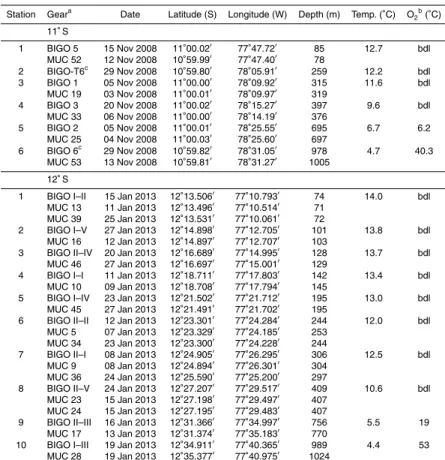
We present data from 6 stations along 11◦S sampled during expedition M77 (cruise

5

legs 1 and 2) in November 2008 and 10 stations along 12◦S during expedition M92

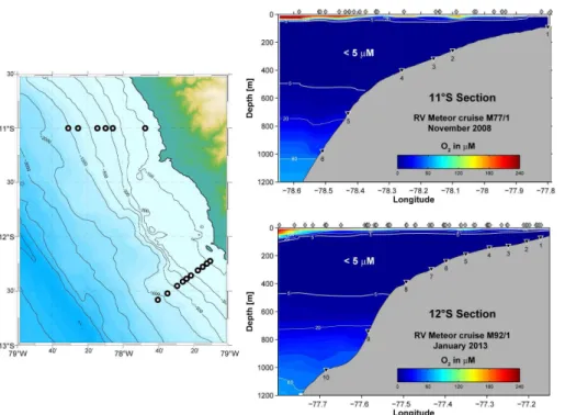
(leg 3) in January/February 2013, both on RV Meteor. Sampling stations are shown

in Fig. 1. Both campaigns took place during austral summer, i.e. the low upwelling season. With the exception of the particulate phases, the geochemical data and benthic

modeling results from the 11◦S transect have been published previously (Bohlen et al.,

10

2011; Scholz et al., 2011; Mosch et al., 2012; Noﬀke et al., 2012). Data from 12◦S are

new to this study.

In situ fluxes were measured using data collected from Biogeochemical Observato-ries, BIGO (Sommer et al., 2008; Sommer et al., unpub. data). BIGO landers contained

two circular flux chambers (internal diameter 28.8 cm, area 651.4 cm2). One lander at

15

11◦S, BIGO-T, contained only one benthic chamber. Each chamber was fitted with an

optode to monitor dissolved O2concentrations. A TV-guided launching system allowed

smooth placement of the observatories at selected sites on the sea floor. Two hours after the landers were placed on the sea floor, the chamber(s) were slowly driven into

the sediment (∼30 cm h−1). During this initial period, the water inside the flux chamber

20

was periodically replaced with ambient bottom water. After the chamber was fully driven into the sediment, the chamber water was again replaced with ambient bottom water to flush out solutes that might have been released from the sediment during chamber in-sertion. The water volume enclosed by the benthic chamber ranged from 8.5 to 18.5 L. During the BIGO-T experiments, the chamber water was replaced with ambient bottom

(8)

BGD

11, 13067–13126, 2014

Peruvian margin

A. W. Dale et al.

Title Page

Tables Figures

◭ ◮

Back Close

Full Screen / Esc

Discussion

P

a

per

|

Discus

sion

P

a

per

|

Discussion

P

a

per

|

Discussion

P

a

per

|

water half way through the deployment period to restore outside conditions and then re-incubated.

Four (11◦S) or eight (12◦S) sequential water samples were removed periodically with

glass syringes (volume of each syringe∼47 mL) to determine fluxes of solutes across

the sediment–water interface. For BIGO-T, 4 water samples were taken before and after

5

replacement of the chamber water. The syringes were connected to the chamber us-ing 1 m long Vygon tubes with an internal volume of 6.9 mL. Prior to deployment, these tubes were filled with distilled water, and great care was taken to avoid enclosure of air bubbles. Concentrations were corrected for dilution using measured chloride

concen-trations in the syringe and bottom water. Water samples for measurements ofpCO₂

10

(12◦S) were taken at four regular time intervals using 80 cm long glass tubes

(inter-nal volume ca. 15 cm3). An additional syringe water sampler (four or eight sequential

samples) was used to monitor the ambient bottom water. The sampling ports for am-bient seawater were positioned 30–40 cm above the seafloor. The incubations were conducted for time periods ranging from 17.8 to 33 h. Immediately after retrieval of the

15

observatories, the water samples were transferred to the onboard cool room (8◦C) for

further processing and sub-sampling.

Sediment samples for analysis were taken using both MUC and BIGO technolo-gies. In this paper we report on MUC data only since the core length (ca. 20–40 cm) was typically much greater than the short BIGO cores (ca. 10 cm). Furthermore, MUC

20

data are unaﬀected by possible artifacts arising from insertion of the roller underneath

the chambers at the end of the BIGO deployments. Retrieved cores were immediately

transferred to a cool room onboard at 4◦C and processed within a few hours.

Sub-sampling for redox sensitive constituents was performed under anoxic conditions using an argon-filled glove bag. Sediment samples for porosity analysis were transported to

25

the onshore laboratory in air-tight containers at 4◦C. Sediment sections for porewater

extraction were transferred into tubes pre-flushed with argon gas and subsequently centrifuged at 4500 rpm for 20 min. Prior to analysis, the supernatant porewater was

(9)

cen-BGD

11, 13067–13126, 2014

Peruvian margin

A. W. Dale et al.

Title Page

Tables Figures

◭ ◮

Back Close

Full Screen / Esc

Discussion

P

a

per

|

Discus

sion

P

a

per

|

Discussion

P

a

per

|

Discussion

P

a

per

|

trifugation tubes with the remaining solid phase of the sediment were stored at−20◦C

for further analysis onshore. Additional samples for bottom water analysis were taken from the water overlying the sediment cores.

3.2 Analytical details

Dissolved oxygen concentrations in the water column were measured using a Seabird

5

SBE43 sensor mounted on a SeaBird 911 CTD rosette system. The optodes were calibrated by vigorously bubbling filtered seawater from the bottom water at each sta-tion with air and with argon for 20 min. The sensors were calibrated against discrete samples collected from the water column on each CTD cast and analyzed onboard

using Winkler titration with an onboard detection limit of ca. 5 µM. However, O2

con-10

centrations at sub-micromolar levels were measured within the core of the OMZ using microsensors (Kalvelage et al., 2013). For the purposes of this study, therefore, we

broadly define O2 concentrations below the detection limit of the Winkler analysis as

anoxic.

Ammonium (NH+₄), nitrite (NO−₂), dissolved ferrous iron (Fe2+), phosphate (PO3₄−)

15

and dissolved sulfide (H2S) were measured onboard using standard photometric

tech-niques with a Hitachi U2800 photometer (Grassho_ﬀet al., 1999). Aliquots of porewater

were diluted with O2-free artificial seawater prior to analysis where necessary.

Pore-water samples for Fe2+ analysis were treated with ascorbic acid directly after filtering

(0.2 µm) inside the glove bag. Detection limits for NO−₃, NH+₄ and TH₂S were 1 µM, 5 µM

20

for PO3₄− and 0.1 µM for NO−₂. Total alkalinity (TA) was determined onboard by direct

titration of 1 mL porewater with 0.02 M HCl using a mixture of methyl red and

methy-lene blue as indicator and bubbling the titration vessel with Ar gas to strip CO2 and

H₂S. The analysis was calibrated using IAPSO seawater standard, with a precision

and detection limit of 0.05 meq L−1. Ion chromatography (Methrom 761) was used to

25

determine sulfate (SO2₄−) in the onshore laboratory with a detection limit of <100 µM

(10)

BGD

11, 13067–13126, 2014

Peruvian margin

A. W. Dale et al.

Title Page

Tables Figures

◭ ◮

Back Close

Full Screen / Esc

Discussion

P

a

per

|

Discus

sion

P

a

per

|

Discussion

P

a

per

|

Discussion

P

a

per

|

and relative accuracy as given by Haﬀert et al. (2013). Analytical details of dinitrogen

gas (N2) measurements, used a model constraint on benthic N turnover, are described

by Sommer et al. (unpub. data).

Partial pressure of CO₂ (pCO₂) was analyzed in the benthic chambers at 12◦S.

pCO2 analysis was performed onboard by passing the sample from the glass tubes

5

(without air contact) through the membrane inlet of a mass spectrometer (GAM200 IPI Instruments, Bremen). The samples were analyzed sequentially by switching from one tube to another and flushed with distilled water between samples. Standards were prepared by sparging filtered seawater from the bottom water from each station using

standard bottles of CO₂of known concentration at in situ temperature for 30 min. The

10

relative precision of the measurement was<1 %.

Wet sediment samples for analysis of POC, PON and total particulate sulfur (TPS) were freeze-dried in the onshore laboratory and analyzed using a Carlo-Erba element analyzer (NA 1500). POC content was determined on the residue after acidifying the

sample with HCl to release the inorganic components as CO2. Inorganic carbon was

15

determined by weight diﬀerence. The precision and detection limit of the analysis was

0.04 and 0.05 dry weight percent (%), respectively. Porosity was determined in the

onshore laboratory from the weight diﬀerence of the wet and freeze-dried sediment.

Values were converted to porosity (water volume fraction of total sediment)

assum-ing a dry sediment density of 2 g cm−3 (Böning et al., 2004) and seawater density of

20

1.023 g cm−3.

Additional samples from adjacent MUC liners taken from the same cast were used for

the determination of down-core profiles of unsupported210Pb_xs (excess) activity.

Be-tween 5 and 34 g of freeze-dried and ground sediment, each averaging discrete 2 cm depth intervals, was embedded into a 2-phase epoxy resin (West System Inc.).

Follow-25

ing Mosch et al. (2012), a low-background coaxial Ge(Li) planar detector (LARI,

Univer-sity of Göttingen) was used to measure total210Pb via its gamma peak at 46.5 keV and

226

Ra via the granddaughter214Pb at 352 keV. Prior to analysis, the gas-tight

(11)

BGD

11, 13067–13126, 2014

Peruvian margin

A. W. Dale et al.

Title Page

Tables Figures

◭ ◮

Back Close

Full Screen / Esc

Discussion

P

a

per

|

Discus

sion

P

a

per

|

Discussion

P

a

per

|

Discussion

P

a

per

|

weeks. In order to determine the unsupported fraction (210Pbxs), the measured total

210

Pb activity of each sample was corrected by subtracting its individual226Ra activity,

assuming post-burial closed system behavior. The relative error of the measurements

(2σ) ranged between 8 and 58 %. Uncertainty of the calculated 210Pbxs data derives

from the individual measurement of210Pb and 226Ra activities according to standard

5

propagation rules. The down-core decrease in 210Pbxs and sediment porosity allows

the determination of sediment accumulation and bioturbation rates (see below). For some cores, the radiometric lead chronology was validated with the detection of the

anthropogenic enrichment peak of nuclide 241Am (co-analysed on 60 keV) as an

in-dependent time marker in the profiles, originating from nuclear tests in the Southern

10

Hemisphere during the early 1960s (data not shown).

3.3 Calculation of dissolved inorganic carbon (DIC) fluxes

DIC concentrations in the benthic chambers at 12◦S were calculated from the

con-centrations of TA andpCO₂using the equations and equilibrium coeﬃcients given by

Zeebe and Wolf-Gladrow (2001).pCO2 and TA concentrations increased linearly with

15

time inside the chambers and there were no spurious outliers such that all

measure-ments were used. Since four samples forpCO₂ were taken using the glass tubes vs.

eight samples for TA analysis in the syringes, each successive pair of TA data were av-eraged for calculating DIC. A constant salinity of 35 (psu), total boron concentration of

0.418 mM and seawater density of 1.025 kg L−1were assumed. Corrections were made

20

for the occurrence of free hydrogen sulfide in the bottom water at the shelf stations. DIC fluxes were calculated from the concentrations as described above.

3.4 Determination of sediment accumulation rates

Particle-bound210Pbxs is subject to mixing in the upper sediment layers by the

move-ment of benthic fauna. The distribution of210Pbxs can thus be used to determine

bio-25

(12)

BGD

11, 13067–13126, 2014

Peruvian margin

A. W. Dale et al.

Title Page

Tables Figures

◭ ◮

Back Close

Full Screen / Esc

Discussion

P

a

per

|

Discus

sion

P

a

per

|

Discussion

P

a

per

|

Discussion

P

a

per

|

simulated the activity of210Pbxs in Bq g

−1

using a steady state numerical model that includes terms for sediment burial, mixing (bioturbation), compaction and radioactive decay:

(1−ϕ(x))·ρ·∂

210

Pbxs(x)

∂t =

∂

(1−ϕ(x))·ρ·D_B(x)·∂

210_Pb

xs(x)

∂x

−

∂(1−ϕ(x))·ρ·v_s(x)·210Pbxs(x)

∂x +(1−ϕ(x))·ρ·λ· 210

Pbxs(x)

(1)

5

In this equation, t (yr) is time, x (cm) is depth below the sediment–water interface,

ϕ(x) (dimensionless) is porosity, vs(x) (cm yr

−1

) is the burial velocity for solids, DB(x)

(cm2yr−1) is the bioturbation coeﬃcient, λ (0.03114 yr−1) is the decay constant for

210

Pbxsandρis the bulk density of solid particles (2.0 g cm

−3

, Böning et al., 2004). Porosity was described using an exponential function assuming steady-state

com-10

paction:

ϕ(x)=ϕ(L)+(ϕ(0)−ϕ(L))·exp

− x

zpor

(2)

where ϕ(0) is the porosity at the sediment–water interface, ϕ(L) is the porosity of

compacted sediments andzpor(cm) is the porosity depth attenuation coeﬃcient. These

parameters were determined from the measured data at each station (Table S2).

15

Sediment compaction was considered by allowing the sediment burial velocity to decrease with sediment depth:

vs(x)=

ωacc·(1−ϕ(L))

1−ϕ(x) (3)

(13)

BGD

11, 13067–13126, 2014

Peruvian margin

A. W. Dale et al.

Title Page

Tables Figures

◭ ◮

Back Close

Full Screen / Esc

Discussion

P

a

per

|

Discus

sion

P

a

per

|

Discussion

P

a

per

|

Discussion

P

a

per

|

The decrease in bioturbation intensity with depth was described with a Gaussian-type function (Boudreau, 1996):

D_B(x)=D_B(0)·exp − x

2

2·x2_s

!

(4)

whereDB (0) (cm

2

yr−1) is the bioturbation coeﬃcient at the sediment–water interface

andxs(cm) is the bioturbation halving depth.

5

The flux continuity at the sediment surface serves as the upper boundary condition:

F(0)=(1−ϕ(0))·ρ· v_s(0)·210Pb_xs(0)·D_B(0)· ∂

210

Pb_xs(x)

∂x

₀

!

(5)

whereF(0) is the steady-state flux of210Pbxs to the sediment surface (Bq cm

−2

yr−1).

The influx of210Pbxswas determined from the measured integrated activity of

210

Pbxs

multiplied byλ:

10

F(0)=λ·ρ

∞

Z

0 210

Pbxs(x)·(1−ϕ(x)) dx (6)

210

Pbxswas present down to the bottom of the core at the 74 m station (12

◦

S), implying

rapid burial rates. Here,F(0) was adjusted until a fit to the data was obtained.

A zero gradient (Neumann) condition was imposed at the lower boundary at 50 cm

(100 cm for the shallowest stations at 12◦S). At this depth, all210Pbxswill have decayed

15

for the burial rates typical of the Peruvian margin. The model was initialized using low

and constant values for210Pb_xsin the sediment column. Solutions were obtained using

(14)

BGD

11, 13067–13126, 2014

Peruvian margin

A. W. Dale et al.

Title Page

Tables Figures

◭ ◮

Back Close

Full Screen / Esc

Discussion

P

a

per

|

Discus

sion

P

a

per

|

Discussion

P

a

per

|

Discussion

P

a

per

|

The adjustable parameters (ωacc,DB(0),xs) were constrained by fitting the

210

Pbxs

data. The goodness-of-fit was done visually since the sampling resolution and

vari-ability in the210Pb_xs do not warrant more rigorous statistical approaches. Model

sen-sitivity analysis indicated thatωacc are accurate to within±20 %. Note, however, that

the uncertainty inωacc due the natural sediment heterogeneity may be equivalent to

5

or larger than this value (Turnewitsch et al., 2000). Unsupported210Pb measurements

were not made at the 101 and 244 m station (12◦S) and sedimentation rates here

were estimated from adjacent stations. Parameters and boundary conditions for

sim-ulating 210Pb_xs at 12◦S are given in Table S2. Results for 11◦S are given by Bohlen

et al. (2011).

10

3.5 Diagenetic modeling of POC degradation

A steady-state 1-D numerical reaction–transport model was used to simulate the

degra-dation of POC in surface sediments at all stations. The model developed for 12◦S is

based on that used to quantify benthic N fluxes at 11◦S by Bohlen et al. (2011) with

modifications to account for benthic denitrification by foraminifera (Dale et al., unpub.

15

data). The methodology used to constrain the POC degradation rates is the same in both studies. A full description of the model can be found in those publications.

The basic model framework follows Eq. (1) i.e. simulating the distribution of dissolved and solid components by considering transport pathways and reactions. Solutes were

transported by molecular diﬀusion and sediment accumulation (burial). Solids were

20

transported by burial and bioturbation, taken from the210Pbxsmodel. Non-local

trans-port rates of solutes by burrowing organisms (bioirrigation) were very low yet included

nonetheless. Solutes simulated include O2, NO

−

3, NO

−

2, NH

+

4, N2, H2S, SO

2−

4 , Fe 2+_,

DIC and methane (CH4). Solids include POC, PON, adsorbed NH+4, reactive iron

(oxy-hydr)oxides and total particulate sulfur. Porewater TA concentrations were not modeled

25

(15)

BGD

11, 13067–13126, 2014

Peruvian margin

A. W. Dale et al.

Title Page

Tables Figures

◭ ◮

Back Close

Full Screen / Esc

Discussion

P

a

per

|

Discus

sion

P

a

per

|

Discussion

P

a

per

|

Discussion

P

a

per

|

using the explicit conservative expression (Wolf-Gladrow et al., 2007), as described in Bohlen et al. (2011).

The model includes a comprehensive set of redox reactions that are ultimately driven by POC mineralization. POC was degraded by aerobic respiration, denitrifi-cation, iron oxide reduction, sulfate reduction and methanogenesis. Manganese

ox-5

ide reduction was not considered due to negligible total manganese in the sediment (Böning et al., 2004; Bohlen et al., 2011). The rate of each carbon degradation path-way was determined using Michaelis–Menten kinetics based on traditional approaches (e.g. Boudreau, 1996). DIC is produced by POC degradation only, that is, no carbonate dissolution and precipitation (see Sect. 4).

10

The total rate of POC degradation was constrained using a novel N-centric approach

based on the relative rates of transport and reactions that produce/consume NH+₄. The

procedure follows a set of guidelines that is outlined fully in Bohlen et al. (2011). The

modeled POC mineralization rates for 11◦S were constrained using both porewater

concentration data and in situ flux measurements of NO−₃, NO−₂ and NH+₄. Dissolved

15

O2 flux data were used as an additional constraint at the deeper stations. The POC

degradation rates at 12◦S were further constrained from the measured DIC and N₂

fluxes. The model output includes concentration profiles, benthic fluxes and reaction rates which are assumed to be in steady-state. Note, however, that the bottom waters

on the inner shelf were temporarily depleted in NO−₃ and NO−₂ at the time of sampling

20

due a trapped body of water close to the coast. Although this leads to uncertainties in

the rate of nitrate uptake byThioploca, POC degradation rates remain well-constrained

from the DIC fluxes.

The model was solved in the same way as described for210Pbxs. The sediment depth

was discretized over an interval ranging from 50 to 100 cm depending on the station

25

(16)

BGD

11, 13067–13126, 2014

Peruvian margin

A. W. Dale et al.

Title Page

Tables Figures

◭ ◮

Back Close

Full Screen / Esc

Discussion

P

a

per

|

Discus

sion

P

a

per

|

Discussion

P

a

per

|

Discussion

P

a

per

|

depth) with a mass conservation >99 %. The importance of time-variable boundary

conditions is discussed below.

3.6 Pelagic modeling of primary production

Primary production was estimated using the high-resolution physical-biogeochemical model (ROMS-BioEBUS) in a configuration developed for the Eastern Tropical Pacific

5

(Montes et al., 2014). ROMS-BioEBUS consists of a hydrodynamic model ROMS (Re-gional Ocean Model System; Shchepetkin and McWilliams, 2003) coupled with the

BIOgeochemical model developed for theEasternBoundaryUpwellingSystems

(BioE-BUS, Gutknecht et al., 2013). BioEBUS describes the pelagic distribution of O2 and

the nitrogen cycle with twelve compartments: phytoplankton and zooplankton split into

10

small (flagellates and ciliates, respectively) and large (diatoms and copepods,

respec-tively) organisms as well as detritus, dissolved inorganic N (NO−₃, NO−₂, and NH+₄),

dissolved organic N (DON) and a parameterization to determine nitrous oxide (N2O)

production (Suntharalingam et al., 2000, 2012). N cycling under a range of redox con-ditions is simulated (e.g. Yakushev et al., 2007).

15

The model configuration covers the region between 4◦N and 20◦S and from 90◦W

to the west coast of South America. The model horizontal resolution is 1/9◦(ca. 12 km)

and has 32 vertical levels that are elongated toward the surface to provide a better rep-resentation of shelf processes. The model was forced by heat and freshwater fluxes de-rived from COADS ocean surface monthly climatology (Da Silva et al., 1994) and by the

20

monthly wind stress climatology computed from QuikSCAT satellite scatterometer data (Liu et al., 1998). The three open boundary conditions (northern, western and south-ern) for the dynamic variables (temperature, salinity and velocity fields) were extracted from the Simple Ocean Data Assimilation (SODA) reanalysis (Carton and Giese, 2008). Initial and boundary conditions for biogeochemical variables were extracted from the

25

CSIRO Atlas of Regional Seas (CARS 2009, http://www.cmar.csiro.au/cars; for NO−₃

and O₂) and SeaWiFS (O’Reilly et al., 2000; for chlorophyll a). Other biogeochemical

(17)

BGD

11, 13067–13126, 2014

Peruvian margin

A. W. Dale et al.

Title Page

Tables Figures

◭ ◮

Back Close

Full Screen / Esc

Discussion

P

a

per

|

Discus

sion

P

a

per

|

Discussion

P

a

per

|

Discussion

P

a

per

|

Monthly chlorophyll climatology from SeaWIFS (Sea-Viewing Wide-Field Sensor) was used to generate phytoplankton concentrations which were then extrapolated vertically from the surface values using the parameterization of Morel and Berthon (1989). Based on Koné et al. (2005), a cross-shore profile following in situ observations was applied to the zooplankton with increasing concentrations onshore.

5

The simulation was performed over an 18 year period. The first 13 years were run considering only the physics and then the biogeochemical model was coupled for the following five years. The coupled model reached a statistical equilibrium after four years. The data presented here correspond to the final simulation year 18. Details of model configuration and validation are described by Montes et al. (2014).

10

For this study, we calculated the primary production (PP) integrated over the

eu-photic zone at the station locations listed in Table 1 for 11◦S and 12◦S. PP (in N units)

was computed as the sum of the new production supported by NO−₃ and NO−₂

up-take and the regenerated production of NH+₄ uptake by nano- and microphytoplankton

(Gutknetch et al., 2013). The atomic Redfield C : N ratio (106/16, Redfield et al., 1963)

15

was used to convert PP into carbon units.

4 Results

4.1 Sediment appearance

Bottom sediments at 12◦S were very similar to those at 11◦S (see Sect. 2). The

sed-iments down to ca. 300 m were typical cohesive, dark-olive anoxic muds found on the

20

shelf and upper slope (Gutiérrez et al., 2009; Bohlen et al., 2011; Mosch et al., 2012). Porewater had a strong sulfidic odor, especially in the deeper layers. Shelf and OMZ

sediments were colonized by mats of large filamentous bacteria, presumablyThioploca

spp. (Gallardo, 1977; Henrichs and Farrington, 1984; Arntz et al., 1991). Surface cov-erage by bacterial mats was 100 % on the shelf and decreased to roughly 40 % by

25

(18)

BGD

11, 13067–13126, 2014

Peruvian margin

A. W. Dale et al.

Title Page

Tables Figures

◭ ◮

Back Close

Full Screen / Esc

Discussion

P

a

per

|

Discus

sion

P

a

per

|

Discussion

P

a

per

|

Discussion

P

a

per

|

was much lower at 11◦S, not exceeding 10 % coverage (Mosch et al., 2012).

Thio-plocatrichomes extended 2 cm into the overlying water to access bottom water NO−₃ (cf. Huettel et al., 1996) and were visible down to a depth of ca. 20 cm at the mat

stations. Despite anoxic bottom waters, no mats were visible at St. 8 (409 m, 12◦S).

Sediments here consisted of hard grey clay underlying a 2–3 cm porous surface layer

5

that was interspersed with cm-sized phosphorite nodules. The upper layer contained large numbers of live foraminifera that were visible to the naked eye (J. Cardich et al.,

unpub. data). Similar foraminiferal “sands” were noted at 11◦S, in particular below the

OMZ. Phosphorite sands on the Peruvian margin are found where enhanced sediment reworking and winnowing takes place due to dissipation of internal wave energy on the

10

seafloor (Suess, 1981; Glenn and Arthur, 1988; Mosch et al., 2012).

4.2 Sediment mixing and accumulation rates

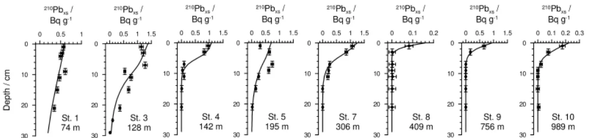
At most stations,210Pbxs distributions decreased quasi-exponentially and showed

lit-tle evidence of intense, deep mixing by bioturbation (Fig. 2 and Bohlen et al., 2011); a feature that is supported by the lack of large bioturbating organisms in and below

15

the OMZ (Mosch et al., 2012). The highest bioturbation coeﬃcient determined by the

model was 4 cm2yr−1 for St. 3 at 12◦S (Table S2). Because megafauna were absent

during fieldwork, the non-zero mixing rates probably reflect the intermittent colonization by fauna that takes place during periodic oxygenation events (Gutiérrez et al., 2008).

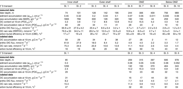
Mass accumulation rates derived from 210Pb_xs modeling were similar to values

re-20

ported previously (Reimers and Suess, 1983c). Rates were extremely high at the

shal-lowest stations (1200 and 1800 g m−2yr−1at 11 and 12◦S, respectively); a factor of 2–3

times higher than measured elsewhere on the transects and 3–4 times higher than the

global shelf average of 500 g m−2yr−1 (Burwicz et al., 2011). They corresponded to

sedimentation rates of 0.45 and 0.3 cm yr−1(Table 2). Beyond the inner shelf, the

sed-25

imentation rates (ωacc) showed much more variability at 12

◦

S than at 11◦S, although

(19)

BGD

11, 13067–13126, 2014

Peruvian margin

A. W. Dale et al.

Title Page

Tables Figures

◭ ◮

Back Close

Full Screen / Esc

Discussion

P

a

per

|

Discus

sion

P

a

per

|

Discussion

P

a

per

|

Discussion

P

a

per

|

accumulation rates of 44 g m−2yr−1 were calculated for St. 8 at 12◦S where erosion

occurs.

4.3 Geochemistry

Dissolved O2concentrations in the water column reveal the vertical extent of the OMZ

and the presence of oxygen-deficient water overlying the upper slope sediments at

5

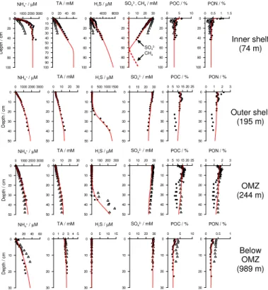
both latitudes (Fig. 1). Qualitatively, geochemical solute profiles from 11 and 12◦S are

typical for continental margin settings (Bohlen et al., 2011; Fig. 3). Sediment porewater

concentrations of NH+₄ and alkalinity were highest on the shelf and decreased with

water depth. Conversely, SO2₄− depletion was more extensive at the shallower stations.

SO2₄− also showed a much stronger depletion on the shelf at 12◦S compared to 11◦S,

10

leading to the formation of a methanogenic layer below 65 cm. The model was able to accurately simulate the geochemical profiles along both transects at all stations (Fig. 3 and Bohlen et al., 2011).

Sulfate reduction is the dominant organic matter (OM) respiration pathway through-out and below the OMZ (Bohlen et al., 2011). The above trends in porewater

concen-15

trations thus confirm general expectations that less reactive organic material reaches the sea floor as water depth increases (e.g. Suess, 1980; Levin et al., 2002). Indeed, measured DIC fluxes and model results provide independent support for decreasing

POC degradation rates with distance oﬀshore (see Sect. 4.5). The decrease in free

sul-fide in the deeper sediment layers with increasing water depth also fits with this idea.

20

However, sulfide oxidation by Thioploca overprints any obvious relationship between

sulfide accumulation and OM degradation in the upper 20 cm of sediments (Henrichs and Farrington, 1984; Bohlen et al., 2011).

4.4 Organic carbon distributions

Surface POC content at 12◦S was lowest (ca. 5 %) on the inner shelf and below the

25

(20)

BGD

11, 13067–13126, 2014

Peruvian margin

A. W. Dale et al.

Title Page

Tables Figures

◭ ◮

Back Close

Full Screen / Esc

Discussion

P

a

per

|

Discus

sion

P

a

per

|

Discussion

P

a

per

|

Discussion

P

a

per

|

PON showed the same qualitative trends. Maximum POC contents of ca. 17 % were measured inside the OMZ and are typical for the Peruvian margin (Suess, 1981). The relatively low POC content on the inner shelf is somewhat anomalous since one may have expected highest values at the shallowest water depths given the higher primary production (see below) and shorter transit time for organic detritus to reach the seafloor.

5

At the OMZ sites, POC showed a marked change at around 15 to 20 cm depth (Fig. 3) which may reflect the regime shift in the Peruvian OMZ during the little ice age circa 1820 AD postulated by Gutiérrez et al. (2009). These features were also present at the St. 4 and 5 on the outer shelf. The steady-state model does not capture centennial changes in OMZ conditions suggested by the POC profiles. Very similar trends were

10

observed at 11◦S, implying that OM distributions are qualitatively and quantitatively

driven by the same first-order processes at both latitudes.

4.5 DIC fluxes

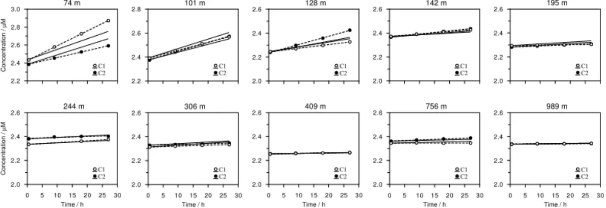
The modeled DIC concentrations inside the benthic chambers at 12◦S showed good

agreement with those calculated from measured TA andpCO2 concentrations (Fig. 4

15

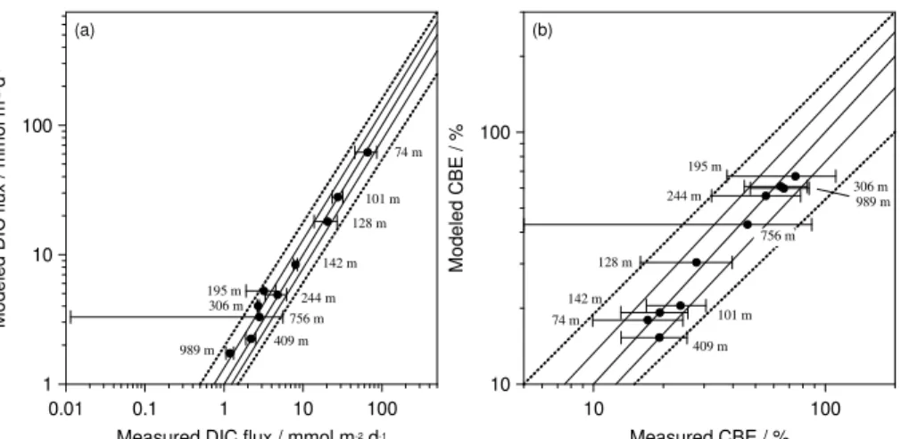
and Table S1). Measured and modeled fluxes agreed to within±50 %, but most stations

were simulated to within±20 % or better (Fig. 5a). It should be remembered that the

model is not only constrained by the DIC fluxes but also by porewater distributions

and benthic DIN and O2 fluxes (Bohlen et al., 2011). Thus, whilst the modeled DIC

fluxes could be improved, they form only one aspect of the overall goodness-of-fit to

20

the observed database. In general, the agreement between the modeled and measured

DIC fluxes aﬀords confidence in the modeled DIC fluxes at 11◦S where in situ pCO2

measurements were not made (Table 2).

Measured DIC fluxes were high on the inner shelf (65.9 mmol m−2d−1) and

de-creased quasi-exponentially with depth (Table 2). DIC fluxes were low in the OMZ

25

at 12◦S (2.2–4.7 mmol m−2d−1) and similar to the deep sites (1.2–2.8 mmol m−2d−1).

The DIC fluxes at 11◦S showed the same trends, although the flux on the inner shelf

(21)

BGD

11, 13067–13126, 2014

Peruvian margin

A. W. Dale et al.

Title Page

Tables Figures

◭ ◮

Back Close

Full Screen / Esc

Discussion

P

a

per

|

Discus

sion

P

a

per

|

Discussion

P

a

per

|

Discussion

P

a

per

|

DIC was assumed to originate entirely from POC mineralization. There was no

clear increase or decrease in Ca2+ and Mg2+ concentration in the benthic chambers

that would indicate an important role for carbonate precipitation/dissolution (data not

shown). This is also inferred from porewater gradients of Ca2+ and Mg2+ at 12◦S

(Fig. S3). Fluxes calculated from the gradients show that the potential contribution of

5

carbonate precipitation was<5 % of the DIC flux across all stations. This is well within

the error of the DIC flux (Table 2), such that carbonate precipitation can be ignored for all practical purposes.

4.6 Organic carbon burial efficiency (CBE)

CBE (%) was calculated using the POC accumulation rates and DIC fluxes, i.e.

10

CBE=POC accumulation rate/(POC accumulation rate+DIC flux)×100 % (Table 2).

CBE is a subjective metric since it depends on the chosen depth where one considers that OM degradation no longer occurs to a significant degree. At the inner shelf and deep stations, POC reaches asymptotic values at around 10 cm (Fig. 3) where organic material is relatively refractive (Reimers and Suess, 1983a). CBE was thus calculated

15

at this depth for these stations. At the OMZ stations, due to variations in POC content in the upper 10 cm, the average POC content in the upper 10 cm was used in the

cal-culations. For St. 8 at 12◦S (409 m), CBE was calculated at 3 cm since the underlying

sediment was old, non-accumulating clay.

We quantified the uncertainty in the CBE calculation based on a 20 % error inωacc

20

and POC content and the di_ﬀerence in DIC fluxes measured simultaneously in two

chambers during each lander deployment (Table 2). The latter arises from the natural “patchiness” of the seafloor and is much greater than the combined analytical error in

the TA andpCO₂measurements. Errors due to artifacts leading from the enclosure of

bottom water by landers are likely to be small (e.g. Hinga et al., 1979). On average,

25

the relative error in DIC flux is the same as that for the POC accumulation rate, around

30 % (Table 2). This leads to a mean relative error in CBE across all stations (at 12◦S)

(22)

BGD

11, 13067–13126, 2014

Peruvian margin

A. W. Dale et al.

Title Page

Tables Figures

◭ ◮

Back Close

Full Screen / Esc

Discussion

P

a

per

|

Discus

sion

P

a

per

|

Discussion

P

a

per

|

Discussion

P

a

per

|

Measured and modeled CBE show very good agreement (Fig. 5b). CBE at 12◦S was

lowest on the inner shelf (<20 %). This contrasts with the organic carbon accumulation

rate which was actually highest here (60 g m−2yr−1; Table 2). Low CBE of 19±6 % were

also observed at the 409 m site due to the low sediment accumulation rate. The highest

CBE was calculated for St. 5 (74±37 %). At 11◦S the modeled range of CBE was very

5

similar yet with a higher shelf value (47 %, Table 2). The maximum CBE of 81 % was calculated for the 695 m station below the OMZ.

4.7 Primary production (PP) and organic carbon rain rate

PP estimates from the ROMS-BioEBUS model for 11 and 12◦S are shown in Fig. 6.

With the exception of the shallowest station, the data represent the annual mean±s.d.

10

for the locations where BIGO landers were deployed. There were no large di_ﬀerences

in PP between the two latitudes and or across the OMZ. For instance, PP increased

from only ca. 80 mmol m−2d−1 at the deepest point to ca. 110 mmol m−2d−1 at the

shallowest. However, the model revealed a much larger intra-annual variability ranging

from ca. 70 to 170 mmol m−2d−1with highest values in austral summer (see Fig. S2).

15

PP was dominated by diatoms at both latitudes.

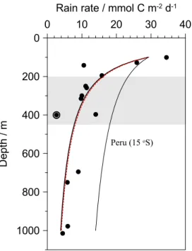
Organic carbon rain rates to the seafloor (RRPOC) were calculated as the sum of the benthic carbon oxidation rate (i.e. DIC flux) and the accumulation rate at 10 cm

(Table 2). RRPOC showed a rapid decrease on the shelf stations at 12◦S with a more

attenuated decrease with depth (Fig. 6a). Station 8 (409 m) at 12◦S is again an

excep-20

tion due to the low POC accumulation there. At 11◦S the trends were not so obvious

due to fewer sampling stations (Fig. 6b). The fraction of PP reaching the sediment in

(23)

BGD

11, 13067–13126, 2014

Peruvian margin

A. W. Dale et al.

Title Page

Tables Figures

◭ ◮

Back Close

Full Screen / Esc

Discussion

P

a

per

|

Discus

sion

P

a

per

|

Discussion

P

a

per

|

Discussion

P

a

per

|

5 Discussion

5.1 Carbon mineralization in the water column

A comparison of the rain rates and PP estimates from the ROMS-BioEBUS model shows that only a minor fraction of PP reaches the seafloor. The true fraction may be even lower since modeled PP is 2 to 3 times lower than the range of 250 to

5

400 mmol m−2d−1 reported previously (Walsh, 1981; Quiñones et al., 2010 and

ref-erences therein). This underestimation may be due to the coarse model spatial

res-olution (1/9◦) which cannot accurately resolve nearshore processes. The model also

represents climatological conditions (i.e. annual mean state), whereas PP measure-ments made during neutral or cold ENSO phases (i.e. La Niña) are likely to higher than

10

the long-term mean (Ryan et al., 2006). The rate at which OM is respired during transit through the water column is usually calculated using sediment trap data (Martin et al.,

1987). The decrease in the sinking flux, F(z), has been widely described using the

following function:

F(z)=F100·(z/100)

−b ₍₇₎

15

whereF100 is the flux at 100 m, z (m) is water depth and b is the dimensionless

at-tenuation coeﬃcient (Martin et al., 1987). A meanb value of 0.86 for oxic open-ocean

waters was derived from the VERTEX program (Martin et al., 1987) and such values

are routinely used in global biogeochemical models (e.g. Dunne et al., 2007).bvalues

lower than 0.86 indicate a slower rate of degradation compared to the mean value and

20

vice-versa.

In the absence of sediment trap data, we estimatedbfor the Peruvian transects by

fitting the modeled rain rates to the following function analogous to Eq. (7):

RRPOC(z)=RRPOC₁₀₁·(z/101)−b (8)

To facilitate comparisons with other studies, the rain rate at the 101 m station at 12◦S

25

(24)

BGD

11, 13067–13126, 2014

Peruvian margin

A. W. Dale et al.

Title Page

Tables Figures

◭ ◮

Back Close

Full Screen / Esc

Discussion

P

a

per

|

Discus

sion

P

a

per

|

Discussion

P

a

per

|

Discussion

P

a

per

|

and excluding the data from St. 8 which is aﬀected by erosion, the best fit to Eq. (8)

is obtained with RRPOC101=28.9±3.2 mmol m

−2

d−1andb=0.88±0.17

(Nonlinear-ModelFit function in MATHEMATICA). The low derived export flux compared to PP rates confirms previous results that most PP in the Humboldt system is mineralized in the surface mixed layer under “normal”, i.e. non-El-Niño, conditions (Walsh, 1981;

5

Gagosian et al., 1983; Quiñones et al., 2010 and references therein).

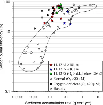
Our derivedb coeﬃcient for the Peruvian OMZ is indistinguishable from the mean

value derived by Martin et al. (1987) for normal oxic waters (Fig. 7). Yet, several stud-ies have shown that respiration of OM in the water column is significantly reduced by

the absence of O₂, leading to elevated carbon fluxes to the lower water column and

10

sediments (Martin et al., 1987; Devol and Hartnett, 2001; Van Mooy et al., 2002). For

example, a coeﬃcient of 0.32 was determined by Martin et al. (1987) for a station 60 km

oﬀshore Peru at 15◦S within the OMZ. Similarly low coeﬃcients (0.36–0.40) have been

reported for the oxygen-deficient Mexican margin (Devol and Hartnett, 2001; Van Mooy

et al., 2002), but not for the Arabian Sea OMZ (0.79±0.11; Berelson, 2001). Van Mooy

15

et al. (2002) supported their findings with laboratory experiments showing that natu-ral particulate material collected at the base of the euphotic zone was degraded less

eﬃciently under anoxic vs. oxic incubation conditions. Given the anoxic water mass

residing on the Peruvian margin, therefore, a much lowerbcoeﬃcient may have been

expected.

20

Devol and Hartnett (2001) observed that rain rates to the seafloor on the Mexican margin, calculated using benthic carbon oxidation rates and burial fluxes at nine sta-tions, showed a very good agreement with sediment-trap estimates. Although some

variability inb within a given oceanic region is to be expected (Berelson, 2001), the

large diﬀerence between our calculatedb value and those previously derived for Peru

25

(25)

BGD

11, 13067–13126, 2014

Peruvian margin

A. W. Dale et al.

Title Page

Tables Figures

◭ ◮

Back Close

Full Screen / Esc

Discussion

P

a

per

|

Discus

sion

P

a

per

|

Discussion

P

a

per

|

Discussion

P

a

per

|

that zooplankton mediate the disaggregation of large organic particulates into slowly-sinking material that is subsequently mineralized by microorganisms. Zooplankton-bacteria interactions may be similarly instrumental in OM breakdown at Peru (this

study), although suﬃcient data is currently lacking to support this idea (Ayón et al.,

2008). Further south oﬀshore Chile, high mineralization rates were indeed linked to

5

a very eﬃcient microbial loop that was closely associated with nanozooplankton

as-semblages (Bottjer and Morales, 2005; Levipan et al., 2007).

Microbial communities adapted to depressed O2levels are also very active

metaboli-cally in the underlying OMZ at Peru (Lam et al., 2009; Kalvelage et al., 2013). High rates

of aerobic heterotrophic respiration have been measured where dissolved O₂

concen-10

trations are in the sub-micromolar range and thus far lower than the detection limit of

the Winkler assay (Kalvelage et al., 2013). Even though O2 is not detectable, it may

nonetheless be transported from the surface ocean to the OMZ interior by diapycnal mixing and rapidly consumed. For instance, diapycnal mixing along the upper conti-nental slope and the lower shelf region of the Mauritanian upwelling supplies around

15

80 mmol m−2d−1 to the underlying oxygen-deficient waters (Brandt et al., 2014). This

exceeds the benthic oxygen uptake by about a factor of 8 (Dale et al., 2014), implying that most of it is consumed in the water column. This mixing also operates on the Pe-ruvian margin and is strongly enhanced due to presence of non-linear internal waves

(M. Dengler, unpub. data). A di_ﬀerent interplay between physical mixing processes and

20

microbial community respiration may well operate at the oﬀshore station at 15◦S where

lowbvalues were determined.

Multi-decadal oscillations in oceanographic conditions may modify particle fluxes in

diﬀerent ways. Martin et al. (1987) conducted their Peru fieldwork in June 1983 which

coincided with a positive El Niño index, that is, a warm phase (http://www.cpc.ncep.

25

noaa.gov). This contrasts with the neutral conditions encountered on our surveys of

11◦S and 12◦S. It is well documented that strong ENSO events alter the ecosystem

functioning oﬀ Peru, and sub-mesoscale zooplankton and anchoveta (Engraulis

(26)

BGD

11, 13067–13126, 2014

Peruvian margin

A. W. Dale et al.

Title Page

Tables Figures

◭ ◮

Back Close

Full Screen / Esc

Discussion

P

a

per

|

Discus

sion

P

a

per

|

Discussion

P

a

per

|

Discussion

P

a

per

|

et al., 2008; Tam et al., 2008). The relative contribution of zooplankton and anchoveta fecal pellets to total carbon export flux is thus expected to vary widely in time and space (Walsh, 1981; Staresinic et al., 1983). This may be of relevance because

sink-ing speeds of zooplankton and anchoveta fecal pellets are very diﬀerent, the latter

being 10 times higher at around 1000 m d−1(Staresinic et al., 1983). It should be noted

5

that anchoveta abundance has also undergone large fluctuations in recent decades,

with total landings being less than 2×106t in the early 1980s (i.e. during Martin

et al.’s (1987) fieldwork) to more than 10×106t in the 2000s (http://www.fao.org).

Zoo-plankton biomass has undergone similar variations, and the two are probably linked (Ayón et al., 2008).

10

There may be other explanations that contribute to the regional di_ﬀerences inb

val-ues related to the approaches used to calculate b. “Bottom-up” (i.e. using sediment

DIC fluxes and POC burial rates) and “top-down” (e.g. sediment traps) approaches

integrate carbon fluxes over very di_ﬀerent time-scales and each su_ﬀer from their own

unique uncertainties. For instance, sediment traps may underestimate the particle flux

15

in water depths<1500 m due to high lateral current velocities (Yu et al., 2001); an

ef-fect likely to be exacerbated on shallower margins (Jahnke et al., 1990). Furthermore, data from a single trap deployment will only capture the settling flux on time-scales

similar to the deployment time. The particle flux measured at 15◦S will thus be biased

towards the productivity and particle dynamics during the eight day period that the trap

20

was operational (Martin et al., 1987). This should raise concerns because PP at 15◦S

shows high temporal variability (Walsh et al., 1981) and the lowbcoeﬃcient there may

be spurious. Particle fluxes in the Arabian Sea also experience high variability due to monsoonal forcing (Haake et al., 1992), and may explain why Berelson (2001) reported

similarbcoeﬃcients to ours for the Arabian Sea instead of lower values. The issue of

25

temporal variability in benthic fluxes is dealt with separately in Sect. 5.4.

Finally, rain rates to the seafloor could be systematically higher than suggested by our data if sediment particles are resuspended and transported down-slope (laterally)