Gilberto de Miranda Junior
models, congested network design models and the integration of both. Location and network design problems arise in several applications of Computer Sci-ence, Engineering and Economy. Nowadays, these problems can not be solved efficiently, what is our major motivation. Established the relevance of these problems, we try to expand their solution frontiers, rewriting them with the aid of flow formulations and using a Benders decomposition framework. Our main goal is to deal with large scale mixed integer programming problems as the
Quadratic Assignment Problem, the Uncapacitated Hub Location Problem and large scale mixed integer nonlinear programming problems. Extensive computa-tional experiments were carried out. The output data is analyzed and discussed, becoming possible to evaluate the quality of the proposed approach
Abstract v
1 Problem Context and Motivation 1
1.1 The Location of Economic Activities . . . 1
1.2 The Local Access Network Design . . . 2
1.3 Facility Location and Network Design . . . 3
2 Assignment Problems 5 2.1 Theory and Background . . . 5
2.2 The Linear Assignment Problem . . . 7
2.3 The Quadratic Assignment Problem . . . 8
2.3.1 Alternative Problem Formulations, Linearizations and Bounds 9 2.3.2 Flow Formulations forQAP . . . 11
2.3.3 A Brief Computational Experiment . . . 12
2.4 Benders Decomposition of the Problem . . . 16
2.4.1 Subproblems . . . 23
2.4.2 Enhancing the Benders Decomposition Algorithm with Flow Equilibrium Constraints . . . 24
2.5 Computational Experiments Using Enhanced Benders Decompo-sition . . . 26
2.6 Concluding Remarks . . . 28
3 The Placement of Electronics with Thermal Effects 33 3.1 Introduction . . . 33
3.2 Thermal Modeling and Temperature Penalty Costs . . . 34
3.2.1 Maximum Temperature and Penalty Costs . . . 35
3.3 Computational Experiments . . . 38
3.3.1 Experiment Description . . . 38
3.3.2 Numerical Results . . . 41
3.4 Concluding Remarks . . . 42
4 The Local Access Network Design With Congestion Costs 47 4.1 Introduction . . . 47
4.2 Multi-commodity Flow Formulation . . . 49
4.2.2 Mixed Integer Nonlinear Program . . . 50
4.2.3 Theoretical Properties of the Linear and the Concave Ver-sions . . . 51
4.2.4 Convexification of Leasing and Congestion Costs . . . 52
4.3 Benders Decomposition of the Problem . . . 53
4.3.1 Problem Manipulations . . . 53
4.3.2 Subproblems . . . 56
4.3.3 Master Problem . . . 59
4.3.4 Algorithm . . . 60
4.3.5 Avoiding Cycles . . . 61
4.4 Computational Results . . . 62
4.5 Conclusions . . . 66
5 Integrating Facility Location and Network Design 69 5.1 Problem Description . . . 69
5.2 Mathematical Programming Formulations . . . 71
5.2.1 Improving the Design of the Local Access Network . . . . 74
5.2.2 Generalized Model Including Hub Transshipment and Net-work Design . . . 77
5.3 Computational Experiences . . . 78
5.3.1 Benders Decomposition for the p-Hub Median Problem and the Uncapacitated Hub Location Problem . . . 78
5.3.2 The Integrated Model: QAP + Local Access Network Design With Congestion Costs . . . 81
5.3.3 Testing the Hub Transshipment Network Design Model . 81 5.4 Concluding Remarks . . . 82
6 Conclusions and Future Work 87 6.1 Contributions . . . 87
6.1.1 The Quadratic Assignment Problem . . . 87
6.1.2 The Placement of Electronics With Thermal Effects . . . 88
6.1.3 The Local Access Network Design With Congestion Costs 88 6.1.4 Integrating Facility Location and Network Design . . . 88
2.2 Perfect matching in a bipartite graph and corresponding network
flow model. . . 6
2.3 Comparison of linear programming bounds for both formulations. 17 2.4 Comparison of lp computing times for both formulations. . . 18
2.5 Comparison of mip computing times for both formulations. . . . 19
2.6 Comparison of mip computing times for both formulations. . . . 20
2.7 Comparison of mip computing times for both formulations. . . . 21
2.8 Comparison of mip computing times for both formulations. . . . 22
2.9 An example of automatic construction of a feasible solution for the dual subproblem. . . 23
2.10 Evolution of computing times withp/qratio. . . 29
2.11 Evolution of computing times withp/qratio. . . 30
2.12 Evolution of computing times withp/qratio. . . 31
3.1 QAP instance and Finite Volume Grid representation. . . 36
3.2 The penalty overheating cost function, for a threshold tempera-ture of 85 Celsius. . . 37
3.3 Evolution of bounds during the method execution. . . 39
3.4 Number of Benders iterations versus p/q cost reason. . . 44
3.5 Execution time [s] versus p/q cost reason. . . 44
3.6 Temperature field for ste36a placement solution without over-heating penalty. . . 45
3.7 Temperature field forste36aplacement solution considering over-heating penalty. . . 45
4.1 The tree network design problem. . . 48
4.2 An example of convexified integrated leasing and congestion cost function. . . 54
5.1 Hub-and-spoke system with different kinds of local access networks. 70 5.2 Possible routes for the commodityij for a givenx=xh. . . . 73
5.3 A city partitioned in regions . . . 84
5.4 A feasible solution . . . 85
parison and respective computing times. . . 13
2.2 Problem dimensions for test instances, number of integer and continuous variables,p/qratio and a comparison of integer mixed programming computing times. . . 14
2.3 Problem dimensions for test instances, number of integer and continuous variables,p/qratio and a comparison of mixed integer programming computing times. . . 15
2.4 Problem dimensions for test instances, number of integer and continuous variables,p/qratio and a comparison of mixed integer programming computing times. . . 16
2.5 Problem dimensions for test instances, number of integer and continuous variables,p/qratio and computing times for Benders decomposition. . . 26
2.6 Problem dimensions for test instances, number of integer and continuous variables,p/qratio and computing times for Benders decomposition. . . 27
2.7 Problem dimensions for test instances, number of integer and continuous variables,p/qratio and computing times for Benders decomposition and flow formulation. . . 28
2.8 Evolution of computing times for Benders algorithm and the flow formulation . . . 30
2.9 Evolution of computing times for Benders algorithm and the flow formulation . . . 31
2.10 Solution of larger instances using the Benders algorithm. . . 32
3.1 Thermo-physical properties for the thermal model. . . 36
3.2 Test instances for computational experiments. . . 40
3.3 Results for computational experiments - first set. . . 41
3.4 Results for computational experiments - second set. . . 42
3.5 Results for computational experiments - third set. . . 43
4.1 Network Dimensions for Test Problems. . . 63
4.2 Average computing time, number of Benders iterations and num-ber of cycle avoiding constraints for experiments 1 to 5. . . 65
ear/linear gap and number of different arcs for experiments 1 to 5. . . 66 4.4 Computing time, number of Benders iterations, number of cycle
avoiding constraints for experiment 6. . . 67 4.5 Computing time, number of Benders iterations, and Nonlinear/linear
gap for experiment 6. . . 68
5.1 Benders decomposition for the p-Hub Median Problem. . . 79 5.2 Benders decomposition for the Uncapacitated Hub Location
Prob-lem. . . 80 5.3 Computational results for the integrated model. . . 81 5.4 Report for a brief experiment using the Hub Transshipment
Motivation
1.1
The Location of Economic Activities
There are important areas of economic analysis in which progress depends of methods for solving or analyzing problems for efficient allocation of indivisible resources. There are practical decision problems that we can cite. For instance, to determine suitable numbers of machine tools of various kinds within a plant, or to define the number of channel capacities and frequencies in telecommuni-cation networks.
Furthermore, indivisibilities in the more highly specialized human or ma-terial factors of production are always at the root of increasing returns to the scale of production. They can arise within the plant or firm, or in relation with a cluster of firms. Strong interest in the effects of indivisibilities comes from the fact that: if industry increasing returns to scale persist at a production level that sizes the total demand in the respective market, we do not have perfect competition and the efficiency of a price system in allocating resources is re-duced. Summarizing, the location theory of economic activities is dependent on the indivisibilities of human and material resources to better explain the reality. This was preconceived by Koopmans and Beckmann [77]. These indivisibilities, by the way, are responsible for some of the greatest mathematical challenges thatMathematical ProgrammingandComputer Sciencehave been facing in the latest 45 years.
It is possible to describe a huge list of practical applications of location problems. Among them, the best location of producers in a multi-commodity transportation network, the best location of warehouses and plants, given the location of his customers and suppliers, the best location of points of inflow or outflow in transportation networks. On the highly competitive economic system created by globalization, it is unnecessary to point out that every single cost component is important: in one side the minimization of production (fixed
or operational)costs improves any organization survivability, at the other side improves the quality of the provided services, maximizing social benefits.
All the systems that have ”hub-and-spoke” features are candidates to loca-tional studies. In a major scale, we can think about the location of private and public facilities to improve the quality of service, and thus quality of life, for a given population. In this context, the facility that we are talking about can be generally called a server, an indivisible resource that is responsible for locally provide access to some kind of commodity for final customers and which is con-nected with other facilities by a transportation network. The commodity being transported from and to these servers can be water, fuel and other petroleum sub-products, electrical energy in power transmission networks, data and other signals in telecommunication and computer networks. The servers can be merely concentrators or complex base stations, depending on the commodity and the transportation technology associated.
Several researchers are dealing with location problems. The work and re-search conducted aroundAssignment Problems, which are some of the simplest approaches to give answers to location theorists, is intensively increasing. The work of Koopmans and Beckmann[77] is a landmark for location theory. For some traditional surveys on this subject, we suggest the work of Motzkin [99], Losch [82], Kuhn [79], Mills [98], Samuelson [121] and Heffley [61]. On the last years, deserve attention the work of Beasley [14], Christofides and Beasley [36], Franca and Luna [45], Mateus and Luna [92], Aikens [2] and Mateus and Thizy [94]. Assignment problems are being studied more recently by Burkard [23], Balas and Saltzman[11], Burkard and Cela [27], Burkard, Cela, Pardalos and Pitsoulis [28], Cela [26], Anstreicher [4], Anstreicher and Brixius [5], Anstreicher, Brixius, Goux and Linderoth [6].
1.2
The Local Access Network Design
problem on a directed graph [85]. In fact, if we neglect variable and congestion costs at the arcs we will have basically the Steiner problem, and in this sense we are treating a N P-Hard problem, for which some computational strategies have been devised [87, 128, 75, 83, 67, 68]. On the other hand, if we neglect fixed and congestion costs on the arcs we have the single source transshipment problem, which can be solved easily [40].
As one can see, it is possible to use this approach to deal with any kind of network flow problem that has a single source tree as optimal solution. The network design problem associated with centralized computer networks and the multiparty multicast tree construction problem are good examples. The last one has been treated with the aid of heuristics [69], but on the two versions pointed by the literature, the Single Source Tree Networks - where we have a true root of the multi-party multicasting tree - and the Core Based Tree Networks - where a single node, the core, is chosen to play a role as the tree root - it is possible to adjust the data to make the model treatment to accomplish the nature of the problem. The provision of multi-point connections is one of most important services that will be required in future broadband communication networks that support distributed multimedia applications. Multimedia video-conference ap-plications, for instance, require that audio and video be transmitted to multiple conference participants simultaneously. This requires that an efficient multi-cast capability be provided by the underlying network. Beyond problems in telecommunications and centralized computer networks, this approach is useful to deal also with petrochemical products distribution networks, water distri-bution networks, and many other local access networks (distributing energy, material resources or signals and data) under mild assumptions.
1.3
Facility Location and Network Design
Network location models have been used extensively to analyze and determine the location of facilities. Classical network models include the location set cov-ering problem [124], the maximum covcov-ering location problem [37] and p-median and p-center problems [60].
In addition to these, the uncapacitated facility location problem[78] has been treated in its own right and is also known assimple plant location problemand
cost as well as a per unit transportation cost, and each node is associated with a fixed charge for building an uncapacitated facility at that node. The objective is to find the network design and the set of facility locations that minimize the total system cost (fixed + operational). This model is reported to be used in the design of pipeline distribution systems, inter-modal transportation systems, power transmission networks and all the hub location problems (that arises in various transportation contexts, and simultaneously address where to locate the hubs and how to design the hub-level network and the access level network).
These models, however, deals with problems were the background assign-ment problem is always a linear one. This means firstly, that no distinction is made between the links used to interconnect facilities and links used to establish the local access network. Here, the location does not presentinterdependency: the definition of a site for one server does not influence the possible assignments for the others. As one can see, none of these two features is much realistic. In many problems involving location of facilities (or servers) and the design of the two underlying networks: the transportation network (established between fa-cilities) and the local access network there are hierarchical considerations to be made. Usually, the technology used to implement the transportation network (larger link capacities and higher traffic velocity) is even different from that used for local access network problems (smaller link capacities and lower traffic velocity).
2.1
Theory and Background
Assignment problems deal with the question of how to assignnitems (jobs,students) tonother items (machines, tasks). Their underlying structure is anassignment
which is nothing else than a bijective mapping φ between two finite sets of n elements. In the optimization problem where we are looking for abestpossible assignment, we have to optimize some objective function which depends on the assignmentφ. Assignments can be represented in different ways. The bijective mapping between two finite setsV and W can be represented in a straightfor-ward way as aperfect matching in a bipartite graphG= (V, W;E), where the vertex sets V and W have, each one, nvertices. Edge (k, i)∈E is an edge of the perfect matching if, and only if, i=φ(k).
After characterizing the setsV andW we get a representation of an assign-ment as apermutation. Every permutationφof the setN= 1, ..., ncorresponds in an unique way to apermutation matrixXφ= (xki) withxki= 1 fori=φ(k)
andxki= 0 fori6=φ(k). This matrixXφcan be viewed as adjacency matrix of
the the bipartite graph Grepresenting the perfect matching, see Figure (2.1).
0 1 0 0
0 0 0 1
0 0 1 0
1 0 0 0
1
2
3
4
1
2
3
4
X
ϕ
=
1 2 3 4
2 4 3 1
ϕ =
Figure 2.1: Different representations of assignments.
The set of all assignments (permutations) ofnitems will be denoted bySn
and has n! elements. This set can be described by the following constraints calledassignment constraints.
n
X
k=1
xki = 1, ∀ i= 1, ..., n (2.1)
n
X
i=1
xki = 1, ∀ k= 1, ..., n (2.2)
xki ∈ {0,1}, ∀ k, i= 1, ..., n. (2.3)
The set of all matricesX= (xki) fulfilling the assignment constraints will be
denoted byXn. When we replace the conditionsxki∈ {0,1}in (2.3) byxki≥0,
we get adoubly stochastic matrix [24]. The set of all doubly stochastic matrices forms the assignment polytope PA. Birkhoff [20] showed that the assignments
correspond uniquely to the vertices ofPA. Thus every doubly stochastic matrix
can be written as convex combination of permutation matrices.
Theorem 2.1.1 (Birkhoff [20]) The vertices of the assignment polytope corre-sponds uniquely to permutation matrices.
Network flows offer another choice of modeling assignments. Let G = (V, W;E) be a bipartite graph with |V| = |W| = n. We embed G in the network N = (N, A, c) with node set N, arc set A and arc capacities c. The node setN consists of a sources, a sinkt and the vertices ofV ∪W, see Figure (2.2).
1
2
3
4
1´
2´
3´
4´
1
1
1
1
1
1
1
1
1
2
3
4
1´
2´
3´
4´
Figure 2.2: Perfect matching in a bipartite graph and corresponding network flow model.
Ford and Fulkerson’s famousMax Flow - Min Cut Theorem [44] states that the value of a maximum flow equals minimum cut value. Such a theorem can be directly translated into the Konig Matching Theorem [76]. Given a bipartite graph G, a vertex cover (cut) in G is a subset of its vertices such that every edge is incident with at least one vertex in the set.
Theorem 2.1.2 (Konig Matching Theorem [76]) In a bipartite graph, the min-imum number of vertices in a vertex cover equals the maxmin-imum cardinality of a matching.
Let us now formulate this theorem in terms of 0-1 matrices. Given a bipartite graphG= (V, W;E) with|V|=|W|=n, we define 0-adjacency matrix Σ of G as a (nxn) matrix Σ = (ςij) by
ςij =
0 if (i, j)∈E
1 if (i, j)∈/E (2.5) A zero cover is a subset of the rows and columns of matrix Σ which contains all 0 elements. A row (column) which is an element of a zero-cover is called a covered row (covered column). Now we get
Theorem 2.1.3 There exists an assignmentφwithςiφ(i)= 0for alli= 1, ..., n, if and only if the minimum zero cover has n elements.
Since a maximum matching corresponds uniquely to a maximum flow in the corresponding networkN, we can construct a zero-cover in the 0-adjacency matrix Σ by means of a minimum cut C in this network: if node i ∈ V of the network does not belong to the cut C, then the row iis an element of the zero-cover. Analogously, if node j ∈ W of the network belongs to the cut C, then column j is an element of the zero-cover.
2.2
The Linear Assignment Problem
activity. The problem is then to find an assignment that makes the profit attainable from the location of facilities as large as possible.
It is clear that this problem is fully defined by its mathematical formula-tion, given below, independently of the locational interpretation. It is useful to remember that this approach gives an artificial picture of locational problems when compared with the complexities and degrees of freedom that can be found in reality. Any kind of rule to subdivide land or allowing the building of more than one plant is not explored, for instance. Other variables like production technology and resource availability are also ignored.
The profitability for then2possible plant location pairs are represented as a square matrix; the element aki representing the fixed profit expected from the
assignment of facilityk to location i. If we choose to use a matrix X = (xki)
to represent the assignment, a linear integer program for the problem can be obtained with the aid of equations (2.1) - (2.3), resulting
maxp=
n
X
k=1
n
X
i=1
akixki (2.6)
subject to (2.1) - (2.3)
This linear integer program has n2 integer variables, and would be a very difficult one, if the linear relaxation of the integrality constraints would not create a set of doubly stochastic matrices. These matrices satisfy the assignment constraints, and from Theorem 2.1.1, these assignments correspond uniquely to the vertices of the associated polytope. This means that, the associated linear program has the same solution as the former integer program, which is a very comfortable property. In fact, Burkard [24] shows that linear assignment problems can be solved by only adding, subtracting and comparing the cost coefficients (see theHungarian Method[79]).
However, if one needs a major level of detail, and requires a better description of reality, it is necessary to improve the model by adding more realistic effects and relationships.
2.3
The Quadratic Assignment Problem
q=X (k,l)
X
(i,j)
bklxkicijxlj (2.7)
We must observe that the transportation cost is independent of the facility assignment and the total demand of intermediate commodities is independent of location assignment. So, the quadratic assignment problem can be stated (in the profitability version)asp−q:
max
n
X
k=1
n
X
i=1
akixki−
n
X
i=1
n
X
j=1
n
X
k=1
n
X
l=1
cijxkibklxlj (2.8)
subject to (2.1) - (2.3)
TheQuadratic Assignment Problem (QAP)remains among the most com-plex combinatorial optimization problems. The inherent difficulty for solving
QAP is also reflected by its computational complexity. Sahni and Gonzalez [120] showed that QAP is N P −Hard and that even finding an approximate solution within some constant factor from the optimal value cannot be done in polynomial time. Recently it has been shown that even local search is hard in some instances, as can be seen in [29] and [107].
2.3.1
Alternative Problem Formulations, Linearizations and
Bounds
There are different, but equivalent, mathematical formulations forQAP which stress different structural characteristics of the problem and lead to different solution approaches. In the form of an integer quadratic program, as stated above, it is very difficult to devise solution strategies. So it is useful to develop techniques to rewriteQAP as an integer linear program.
max n X k=1 n X i=1
akixki−
n X k=1 n X l=1 n X i=1 n X j=1
dkiljykilj (2.9)
subject to (2.1) - (2.3) and:
n
X
j=1
ykilj = xki , ∀i, k, l= 1, ..., n, i6=j, k6=l (2.10)
n
X
l=1
ykilj = xki , ∀i, j, k= 1, ..., n, i6=j, k6=l (2.11)
ykilj = yljki , ∀i, j, k, l= 1, ..., n, i6=j, k6=l, (2.12)
ykilj ≥ 0, ∀i, j, k, l= 1, ..., n, i6=j, k6=l (2.13)
Closely related to some linearizations are the polyhedral studies performed by Barvinok [12], Junger and Kaibel [70],[71] and Padberg and Rijal [106], de-signed to derive theQAP polytope for use withBranch-and-Cut methods. This family of linearizations usually produces strong linear programming relaxations, being on the other hand very difficult to solve. If the good linear programming lower bounds are desirable to obtain success in a Branch-and-Cut framework, the excessive computational cost to solve the programs is really a problem. Even the work of Junger and Kaibel [70],[71], over the linearization of Adams and Johnson[1] demands considerable computational efforts to attain substan-tial results.
Otherwise, many authors have chosen to work with QAP in its original quadratic form. WritingQAP trace formulation, we have:
maxtr(A−CXBT)XT (2.14)
subject to:
X ∈ Xn. (2.15)
The trace formulation was used by Finke, Burkard and Rendl [43] to intro-duce the eigenvalue bounds, a stronger class of lower bounds when compared to bounds obtained via mixed integer linear programming. The eigenvalue lower bounds are, however, very expensive in terms of computational time and dete-riorate quickly when lower levels of the Branch-and-Bound tree are searched. Requirements for a good bound are not to be so hard to compute, be easily evaluated for subsets of the problem which occur after some branching, and, of course, to be tight. Recently, the work of Anstreicher et al. [5] about bounds for
QAPis based onSemi-Definite Programmingrelaxations, and these new bounds are reported to be superior to all the other bounds available from QAP litera-ture. Solutions for large (and hard) QAPLIB instances as ste36a, ste36b and
max n X k=1 n X i=1
akixki −
n X i=1 n X j=1 n X k=1 n X l=1
cijfijkl (2.16)
subject to (2.1) - (2.3) and:
bklxki+
n
X
j=1
fjikl = bklxli+
n
X
j=1
fijkl , ∀ i, k, l= 1, ..., n (2.17)
fiikl = 0, ∀ i, k, l= 1, ..., n (2.18)
fijkl ≥ 0, ∀ i, j, k, l= 1, ..., n (2.19)
This was the first technique proposed to linearizeQAP, due to Koopmans and Beckmann [77], and it works just like the other ones: introducing addi-tional variables and constraints. However, this linearization is very weak, since constraints (2.17) can be satisfied with zero flows between facilities. The linear programming relaxation yields then a trivial solution, consequently producing low quality linear programming lower bounds.
Instead of working with the linearized Koopmans and Beckmann formula-tion, (2.16) - (2.19), we suggest to rewrite constraints (2.17) into two equivalent sets, representing the flow balance at the source and sink points for each com-moditykl:
max n X k=1 n X i=1
akixki−
X
(i,j),i6=j
X
(k,l),k6=l
cijfijkl (2.20)
subject to (2.1) - (2.3) and:
−
n
X
j=1 fkl
ij = −bklxki , ∀ i, k, l= 1, ..., n, i6=j , k6=l (2.21)
n
X
i=1
fijkl = bklxlj , ∀ j, k, l= 1, ..., n, i6=j , k6=l (2.22)
fijkl ≥ 0 , ∀ i, j, k, l= 1, ..., n, i6=j , k6=l (2.23)
variables, andn4−n2+ 2nconstraints. In fact, this formulation is not so strong as the formulation of Adams and Johnson [1], and it is possible to observe some weakness of the linear programming bounds as the problem size increases. On the other hand, this flow formulation is very easy to solve. The idea here is to obtain a well balanced mixed integer programming formulation, which sustain a reasonable linear programming lower bound, being not so difficult to solve as the other ones.
Pursuing this objective, one can add a new family of constraints to the above flow formulation that can make it easier. If the facilitykis located at the sitei and the facilitylis placed at the sitej, constraints (2.21) and (2.22) ensure that the flows from i to j and from j to i equal the demands for the intermediate commodities bkl and blk. So, if xki = 1 and xlj = 1 then −fijkl = −bkl and
−flk
ji =−blk, or simply, forbkl 6= 0:
1
bkl f
kl
ij = 1, ∀ i, j, k, l= 1, ..., n, i6=j , k6=l
1
blk f
lk
ji = 1, ∀ i, j, k, l= 1, ..., n, i6=j , k6=l
yielding:
1 bkl
fijkl =
1 blk
fjilk , ∀ i, j, k, l= 1, ..., n, i6=j , k6=l
and implying:
blk fijkl = bklfjilk , ∀ i, j, k, l= 1, ..., n, i6=j , k6=l (2.24)
These seemingly innocuous constraints are the key to balance the flow for-mulation stated above, equations (2.20) - (2.23), ensuring reasonable linear pro-gramming bounds and yet producing very easy linear programs. In fact, for the symmetric instances one set of flow balance equations, (2.21) or (2.22) can be dismissed. In order to try out all these formulations, comparing linear pro-gramming lower bounds and mixed integer propro-gramming solution time, a set of computational experiments was carried out.
2.3.3
A Brief Computational Experiment
At this point it is useful to discover how the flow formulation will behave, when up against some well documented instances from the literature, available in
rpqaplus the size of the instance.
In Table 2.1, we show a comparison between linear programming bounds obtained by the flow formulation and Adams and Johnson linearization. In despite of the little degeneracy observed in our bounds, they are achieved at a low computing cost. Checking the instances with the higher bounds, it is possible to note that the flow formulation bounds improve quality when dealing with sparse demand matrices. This is not really a surprise, since Heffley [61] has concluded that the presence of sparse demand matrices could lead to integral assignments, when using Koopmans and Beckmann linearization. Because the flow formulation is in some sense derived from Koopmans and Beckmann model, we may expect that this property must be common to both. At this point, it is necessary to remark that in real life applications, one can expect sparse demand matrices instead of dense ones, as the problem size increases. In Figures (2.3) and (2.4) we have the obtained results in graphical form.
QAP LIB Flow Formulation Bound Adams and Johnson Bound Integer instance lp bound time[s] Quality lp bound time[s] Quality Optimal
chr12a 8593.12 1 0.900 9552 725 1.000 9552
chr12b 7184 1 0.737 9742 508 1.000 9742
chr12c 10042.7 1 0.900 11156 1068 1.000 11156
chr15a 8621.94 4 0.871 9513 30146 0.961 9896
chr15c 9504 4 1.000 9504 3622 1.000 9504
had12 894 17 0.541 1621.54 2533 0.982 1652
had14 1300.5 62 0.477 2666.12 14778 0.979 2724
lipa10a 318.8 4 0.674 473 50 1.000 473
nug12 348 10 0.602 522.89 6597 0.905 578
nug15 621 86 0.540 1041 131923 0.905 1150
nug5 49 1 0.980 50 0 1.000 50
nug6 72 0 0.837 86 1 1.000 86
nug7 118 0 0.797 148 3 1.000 148
nug8 154 1 0.720 203.5 17 0.951 214
scr10 21958 2 0.816 26873.1 269 0.998 26922
scr12 25474 5 0.811 29827.3 4555 0.950 31410
tai10a 47953.3 3 0.355 131098 160 0.971 135028
tai10b 855788 1 0.723 1176140 248 0.994 1183760
tai5a 10747 0 0.833 12902 0 1.000 12902
tai6a 21427.8 1 0.728 29432 1 1.000 29432
tai7a 31730.1 0 0.588 53976 1 1.000 53976
tai8a 41952.2 1 0.541 77502 7 1.000 77502
tai9a 41816 2 0.442 93501 37 0.988 94622
Table 2.1: Linear programming bounds for both formulations under comparison and respective computing times.
occupa-tion, competition for locations and other interferences). They also serve as a point of connection with the well established location theory, linear by principle. The idea here is to verify the assumption that, as the p/q ratio increases, our model becomes more competitive. In this context, and since linear profitabil-ity matrices are not available on the instances of QAP LIB, we include linear profitabilitiesp= (P
(k,i)aki) varying from 0 to 10 times the magnitude of the
quadratic transportation cost componentq= (P (i,j)
P
(k,l)cijfijkl), defining the
linear/quadratic ratiop/q. These linear profitabilities were generated randomly with the aid of the standard pseudo-random number generator implemented on the GNU C compiler GCC version 3.0. It may also be observed that because the problems contained inQAPLIB are purely quadratic, there are no difference established between cost and demand matrices. This is not of real importance when dealing with formulations based on Lawler’s linearization (since they pre-multiplybkl andcij), but the flow formulation is not adapted to deal with zero
transportation costs. This was responsible for some additional effort to rebuild the instances in a coherent way.
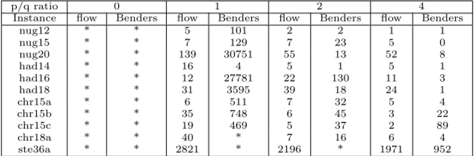
Tables 2.2, 2.3 and 2.4 presents thep/q ratio, and the computing times for the flow formulation and Adams and Johnson [1] linearization (2.9) - (2.13). The entries on Tables 2.2, 2.3 and 2.4 assigned with∗ are describing instances not solved in 24 hours of computation. In order to provide a better insight on analysis, we have plotted these results on Figures (2.5), (2.6), (2.7) and (2.8), in logarithmic scale.
Original Problem Variables p/q Flow form. Adams and Johnson
instance size Integer Continuous ratio time[s] time[s]
esc8a 0 6 146
esc8b 0 15 710
esc8c 8 64 3136 0 14 207
esc8d 0 6 196
esc8e 0 14 176
esc8f 0 5 202
nug6 6 36 900 0 2 1
nug7 7 49 1764 0 4 6
nug8 8 64 3136 0 15 227
rpqa7 7 49 1764 0 9 2
rpqa8 8 64 3136 0 55 83
rpqa9 9 81 5184 0 348 166
tai7a 7 49 1764 0 6 1
tai8a 8 64 3136 0 28 9
tai9a 9 81 5184 0 247 178
tai10a 10 100 8100 0 1197 1218
Table 2.2: Problem dimensions for test instances, number of integer and con-tinuous variables, p/q ratio and a comparison of integer mixed programming computing times.
chr12c 0.314 3 803
chr12c 0.662 4 1217
chr15a 0.631 16 14209
chr15a 0.856 6 10125
chr15b 15 225 44100 0.726 36 77071
chr15b 1.817 14 60452
chr15c 0.944 19 3872
chr15c 0.807 9 3058
chr18a 0.564 116 *
chr18a 18 324 93636 1.304 41 *
chr18b 0.455 21 *
chr18b 1.864 7 *
chr20a 1.047 76 *
chr20a 2.028 28 *
chr20b 20 400 144400 0.824 47 *
chr20b 1.702 10 *
chr20c 1.056 108 *
chr22a 0.304 138 *
chr22a 22 484 213444 0.744 19 *
chr22b 0.293 96 *
chr22b 1.341 18 *
Table 2.3: Problem dimensions for test instances, number of integer and con-tinuous variables, p/q ratio and a comparison of mixed integer programming computing times.
In fact, for the problems with linear installation profitabilities, for some instances it is possible to find the integer optimal solution using our flow formu-lation before the completion of the linear programming solution of Adams and Johnson [1] formulation. The only class of test instances in which the flow for-mulation was defeated was for the instanceshad∗ ∗, just those that has some of the poorest linear programming bounds. In despite of that, the flow formulation lack of performance decreases as the ratiop/qgrows.
These observations clearly suggest the existence of an equilibrium point be-tween the bound quality and the cost to compute it. The natural conclusion here is that Adams and Johnson formulation is so hard to solve that his good linear programming bounds are overcomed by the large computing times required to obtain them. Even in some purely quadratic instances it is possible to defeat Adams and Johnson computing times, as observed in Table 2.2.
We must also consider the solution of the modified versions of the instances nug30 andste36a, reported until now only by Anstreicher et al. [6], using large scale parallel computing. For certain conditions of thep/qratio, these problems could be solved in computing times not superior to one hour, as reported in Table 2.4.
Original Problem Variables p/q Flow form. Adams and Johnson
instance size Integer Continuous ratio time[s] time[s]
had12 0.585 35 14
had12 12 144 17424 1.534 2 3
had12 4.707 2 3
had14 0.464 20 42
had14 14 196 33124 1.312 8 7
had14 2.592 12 8
had16 16 256 57600 0.827 12 16
had16 1.036 12 11
had18 18 324 93636 0.689 209 74
had18 1.590 89 49
lipa10a 2.375 2 1
lipa10a 5.770 1 1
lipa10b 10 100 8100 0.693 6 4
lipa10b 1.440 1 1
lipa10b 2.524 1 1
nug12 2.401 3 110
nug12 12 144 17424 3.621 3 30
nug12 8.584 1 9
nug15 0.990 61 1350
nug15 15 225 44100 1.113 24 258
nug15 2.981 5 94
nug15 5.522 6 126
nug20 0.434 1069 *
nug20 20 400 144400 3.268 42 654
nug20 4.477 80 799
nug30 30 900 756900 0.769 2719 *
nug30 1.358 1779 *
scr10 10 100 8100 0.221 22 311
scr10 0.414 7 95
scr12 12 144 17424 0.188 146 13554
scr12 0.336 54 6854
ste36a 0.843 2896 *
ste36a 36 1296 1587600 1.199 2801 *
ste36a 1.871 2196 *
tai10b 0.003 197 344
tai10b 10 100 8100 0.013 96 714
tai10b 0.023 95 658
Table 2.4: Problem dimensions for test instances, number of integer and con-tinuous variables, p/q ratio and a comparison of mixed integer programming computing times.
2.4
Benders Decomposition of the Problem
Comparison of LP bounds.
0 0,1 0,2 0,3 0,4 0,5 0,6 0,7 0,8 0,9 1
chr12a chr12b chr12c chr15a chr15c had12 had14 lipa10a nug12 nug15 nug5 nug6 nug7 nug8 scr10 scr12 tai10a tai10b tai5a tai6a tai7a tai8a tai9a
Bound Quality
Flow form.
Adams & Johnson 94
Figure 2.3: Comparison of linear programming bounds for both formulations.
that is then followed by the solution strategies of dualization, outer linearization and relaxation.
Starting with the flow formulation described by equations (2.20) - (2.23), from the viewpoint of mathematical programming we can conceive a projection of the problem onto the space of theassignment variablesx, thus resulting the following implicit problem to be solved at a superior level:
min −
n
X
k=1
n
X
i=1
akixki + t(x) (2.25)
subject to (2.1)-(2.3)
Comparison of LP computing times
1 10 100 1000 10000 100000
chr12a chr12b chr12c chr15a chr15c had12 had14 lipa10a nug12 nug15 nug5 nug6 nug7 nug8 scr10 scr12 tai10a tai10b tai5a tai6a tai7a tai8a tai9a
Time[s]
Flow form.
Adams & Johnson 94
Figure 2.4: Comparison of lp computing times for both formulations.
level:
t(x) = min
n
X
i=1
n
X
j=1
n
X
k=1
n
X
l=1
cijfijkl (2.26)
subject to:
−
n
X
j=1
fijkl = −bklxki , ∀ i, k, l= 1, ..., n, i6=j , k6=l (2.27)
n
X
i=1
Comparison of computing times for p/q = 0
1 10 100 1000 10000
esc8a esc8b esc8c esc8d esc8e esc8f nug6 nug7 nug8 rpqa7 rpqa8 rpqa9 tai7a tai8a tai9a tai10a
Time[s]
Flow form.
Adams & Johnson 94
Figure 2.5: Comparison of mip computing times for both formulations.
fkl
ij ≥ 0, ∀ i, j, k, l= 1, ..., n, i6=j , k6=l (2.29)
forxfixed.
The feasibility requirements related to the integer variablesx implies that the facilities for which xki = 1 are such that the superior level solution is an
assignmentbetween the set of facilities and the set of locations. Thus, there is no need for further feasibility constraints on the domain of the projected problem (2.25), and the existence of the minimum in the subproblem (2.26)-(2.29) is ensured since we are minimizing a convex function in a nonempty set.
Since the subproblem has a linear objective function and linear constraints, the Karush-Kuhn-Tucker conditions are necessary and sufficient for optimality. With two associated vectors vkl
Comparison of computing times for p/q > 0
1 10 100 1000 10000 100000
chr12a (0,426) chr12a (0,796) chr12b (0,383) chr12b (0,592) chr12c (0,314) chr12c (0,662) chr15a (0,631) chr15a (0,856) chr15b (0,726) chr15b (1,817) chr15c (0,807) chr15c (0,944)
Time [s]
Flow form.
Adams & Johnson 94
Figure 2.6: Comparison of mip computing times for both formulations.
no duality gap for any xwhich forms an assignment, the optimal value of the subproblem can be written as:
t(x) = max
n
X
k=1
n
X
l=1
n
X
j=1
bklxljvjkl− n
X
k=1
n
X
l=1
n
X
i=1
bklxkiukli (2.30)
subject to:
vkl
j −ukli ≤ cij , ∀ i, j, k, l= 1, ..., n, i6=j, k6=l (2.31)
vklj ∈ R, ∀ j, k, l= 1, ..., n, i6=j, k6=l (2.32)
Comparison of computing times for p/q > 0
1 10 100 1000
had12 (0,585) had12 (1,534) had12 (4,707) had14 (0,464) had14 (1,312) had14 (2,592) had16 (0,827) had16 (1,036) had18 (0,689) had18 (1,59) lipa10a (2,375) lipa10a (5,77) lipa10b (0,693) lipa10b (1,44) lipa10b (2,524)
Time [s]
Flow form.
Adams & Johnson 94
Figure 2.7: Comparison of mip computing times for both formulations.
forxfixed.
At this point, it is interesting to observe that the feasible solution set of the dual subproblem is always the same, independently of the assignment x. So, for every x, the value of the dual objective function underestimates the corresponding primal objective cost. If at a certain cycle h the subproblem has been solved for a given assignment xh
ki the optimal value t(xh) occurs for
vkl j =v
kl,h
j andukli =u kl,h
i and is given by:
t(xh) = n
X
k=1
n
X
l=1
n
X
j=1 bklxhljv
kl,h j −
n
X
k=1
n
X
l=1
n
X
i=1 bklxhkiu
kl,h
i (2.34)
Comparison of computing times for p/q > 0
1 10 100 1000 10000 100000
nug12 (2,401) nug12 (3,621) nug12 (8,584) nug15 (0,99) nug15 (1,113) nug15 (2,981) nug15 (5,522) nug20 (3,268) nug20 (4,477) scr10 (0,221) scr10 (0,414) scr12 (0,188) scr12 (0,336) tai10b (0,003) tai10b (0,013) tai10b (0,023)
Time [s]
Flow form.
Adams & Johnson 94
Figure 2.8: Comparison of mip computing times for both formulations.
is equivalent to the master problem:
min −
n
X
k=1
n
X
i=1
akixki + η (2.35)
subject to (2.1) - (2.3) and:
η ≥
n
X
k=1
n
X
l=1
n
X
j=1
bklxljvkl,hj − n
X
k=1
n
X
l=1
n
X
i=1
2 3 4 5 6 2 3 4 5 6
= u kli + c ij
v kl j
= u kli + c ij
v kl j
= u kli + c ij
v kl j
= u kli + c ij
v kl j
= u kli + c ij
v kl j ukli
− c
u = v kl
j kl i
− c
u = v kl
j kl i
− c
u = v kl
j kl i
− c
u = v kl
j kl i = M ji ji ji ji
Figure 2.9: An example of automatic construction of a feasible solution for the dual subproblem.
2.4.1
Subproblems
For a fixed assignment associated with the matrixxhki, the computation of a
min-imal cost flowt(xh) can be separated in a series of trivial network flow problems,
one for each pairkl. We remark that, for an optimal solution (xh ki, f
kl,h
ij ) for the
primal problem, an associated optimal solution (vjkl,h, ukl,hi ) for the dual sub-problem (2.30) -(2.33) should minimize for eachfkl
ij the correspondent parcel of
the associated Lagrangean function.
This dual problem has many feasible solutions, contrarily to the primal prob-lem that has an unique trivial solution. Since fijkl,h=bkl ifxhki= 1 andxhlj = 1
we have from the complementary slackness condition that:
vjkl,h−u kl,h
i ≤ cij , ∀ i, j= 1, ..., n, i6=j, k6=l
vjkl,h−u kl,h
i = cij , if xhki= 1 and xhlj = 1
In such a way that we can obtain the following dual feasible solution, asso-ciated with the primal solutionfijkl,h(see Figure (2.9)). Fixing a single variable ukl,hi , it is possible to construct:
vjkl,h=u
kl,h
i +cij , ∀ j= 1, ..., n, i6=j, k6=l (2.37)
ukl,hi = maxj , j6=i [vkl,hj −cij], ∀ i= 1, ..., n , i6=j , k6=l (2.38)
The systematic evaluation of the dual variables with meaningful values is a clue for an efficient implementation. Here, the two series of dual variables can be interpreted as price information. Each variablevjkl,h represents the commodity price after flowing from facilitykto facilityl, if facilitylis placed at locationj. The variablesukl,hi represents the commodity price before flowing from facility kto facilityl, if facilitykis placed at locationi.
2.4.2
Enhancing the Benders Decomposition Algorithm
with Flow Equilibrium Constraints
Our task now is to modify the above proposed scheme to accomplish constraints (2.24). It is possible to observe that (2.24) describes a coupling between the flows of commoditiesklandlk. In order to perform the task, it is necessary to point that, for a fixed x=xh, the primal subproblem for commoditieskl and lkis,
fork6=l:
min
n
X
i=1
n
X
j=1
(cijfijkl+cjifjilk)
subject to:
−
n
X
j=1
fijkl = −bklxki, ∀ i= 1, ..., n, i6=j
−
n
X
i=1
fjilk = −blkxlj , ∀ j= 1, ..., n, i6=j
n
X
i=1
fijkl = bklxlj , ∀ j= 1, ..., n, i6=j
n
X
j=1
fjilk = blkxki , ∀ i= 1, ..., n, i6=j
blkfijkl = bklfjilk , ∀ i, j= 1, ..., n, i6=j
fijkl ≥ 0 , ∀ i, j= 1, ..., n, i6=j
fjilk ≥ 0 , ∀ i, j= 1, ..., n, i6=j
The trivial and unique solution of this problem is fkl
ij =bkl and fjilk =blk,
forxki= 1 and xlj = 1, andfijkl = 0 and fjilk = 0 otherwise. This result leads
subject to:
vklj +blkλklij −ukli ≤ cij , ∀ i, j= 1, ..., n , i6=j
vlki −bklλklij −ulkj ≤ cji , ∀ i, j= 1, ..., n , i6=j
vkl
j ∈ R, ∀ j = 1, ..., n, i6=j
ukli ∈ R, ∀ i= 1, ..., n, i6=j
Fixing at a reference value a single variable ukl
i and also a single variable
ulk
j , makingλklij = 0 foriandj such that xhki= 1 andxhlj = 1, it is possible to
write:
vkl,hj =u
kl,h
i +cij , ∀ j= 1, ..., n
vlk,hi =ulk,hj +cji, ∀ i= 1, ..., n
Using the above definedvkl,hj andvilk,h, we have for ukl
i andulkj :
ukl,hi −blkλkl,hij ≥ v
kl,h
j −cij , ∀ i, j= 1, ..., n, i6=j
ulk,hj +bklλkl,hij ≥ v
lk,h
i −cji , ∀ i, j= 1, ..., n, i6=j
We must remark that, an enough high value ofλkl
ij can eventually increase
the value ofukl,hi while eventually decreasing the value of u lk,h
j . The idea here
is to decrease the value of any component of vector u as far as possible, but never increasing the value of another component. Constructing a consistent dual solution we have to fix, for instance, all the components of vectorλh≥0 as high as possible, while maintaining the idea of never increasing of any component of vectoruh:
ukl,hi = maxj , j6=i [vjkl,h−cij], ∀ i= 1, ..., n , i6=j
And determiningλkl,hij in such way that:
λkl,hij = 0 for index j that maximizes v kl,h j −cij
λkl,hij =
1 blk(u
kl,h i −v
kl,h
j +cij), ∀ i, j= 1, ..., n, i6=j
ulk,hj = maxi , i6=j [vilk,h−bklλkl,hij −cji], ∀ i= 1, ..., n, i6=j
Now, we are ready to try out our decomposition algorithm over a set of instances, object of the next section.
2.5
Computational Experiments Using Enhanced
Benders Decomposition
These experiments follows the same standards and adopted convention used to compare the flow formulation and Adams and Johnson formulation [1]. The tests were carried out in a Sun Blade 100 with one 500 MHz Ultra-SPARC processor and 1 Gbyte of RAM memory. The operational system is Solaris 5.8. The Benders decomposition algorithm was implemented in C++ withCPLEX 7.0 application programming interface called ILOG Concert Technology. To perform the tests, instances fromQAPLIB, by Burkard, Karish and Rendl [29], with sizes fromn= 8 ton= 36 were selected. TheQAPLIB instances selected to make part of the test, are shown in Tables 2.5 and 2.6. We have solved purely pseudo-random instances, in the same range of sizes. These random instances are not Koopmans and Beckmann instances, since they do not sustain the triangular inequality, and are represented by names beginning with rpqa plus the size of the instance. We are setting profitabilities to install a facility in a given location, fromp/q= 0 top/q= 16. Tables 2.5 and 2.6 presents thep/q ratio, and the computing times for the Benders decomposition algorithm.
Original Problem Iterations Variables p/q Benders algorithm
instance size h Integer Continuous ratio time[s]
esc8a 8 82 64 3136 0 473
nug5 5 33 25 400 0 11
nug6 6 188 36 900 0 1266
nug12 12 102 144 17424 1.810 663
23 3.621 11
31 3.621 26
nug15 15 11 225 44100 4.881 2
15 6.303 5
63 1.258 661
nug20 20 13 400 144400 3.992 11
9 4.477 2
rou12 12 99 144 17424 2.630 199
ste36a 36 108 1296 1587600 3.853 1381
40 5.780 108
tai5a 5 45 25 400 0 14
tai6a 6 188 36 900 0 1071
tai7a 7 657 49 1764 0 90437
Table 2.5: Problem dimensions for test instances, number of integer and con-tinuous variables,p/qratio and computing times for Benders decomposition.
53 2.680 136
rpqa16 16 33 256 57600 2.701 53
19 2.752 12
20 4.158 12
15 4.400 6
20 4.508 12
17 4.583 8
74 3.261 821
40 4.483 124
42 4.496 146
36 4.598 101
31 4.731 72
30 4.771 63
rpqa25 25 21 625 360000 5.194 30
21 5.381 29
11 5.767 6
26 5.801 40
15 5.816 11
20 6.071 22
15 6.377 11
21 3.037 5
rpqa9 9 6 81 5184 7.594 0
5 11.071 0
3 15.189 0
Table 2.6: Problem dimensions for test instances, number of integer and con-tinuous variables,p/qratio and computing times for Benders decomposition.
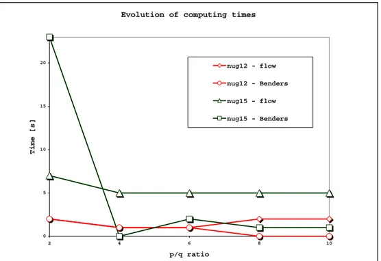
Tables 2.8 and 2.9 presents an evolution of the computing times for Benders decomposition algorithm and for our monolithic implementation. These results are plotted in Figures (2.10), (2.11) and (2.12).
As one can see, the computing times for the flow formulation monolithic implementation are sometimes better than those obtained by Benders decom-position scheme. The exception occurs on the situations that we deal with the larger instances, with higherp/qratios. This effect is due to the master problem strengthening, that accelerates the lower bound progression.
We can sustain that high p/q ratios better describe the cost structure of real large scale implementations, and that the linear parcel, that represents the profitability of a given location, can be considered in some cases more important than the transportation costs, from the economic point of view. This is specially true when we think in location theory, since the linear term gives the profitability of a location for an economic activity. The economic equilibrium condition is so found for p/q= 1, and all situations wherep/q >1 capture liquid profit for the considered optimal location for at least one activity. It is necessary to make clear that our objective, when we start to develop the decomposition scheme, was to go were no one has gone before: proceed with the solution of larger instances. This is impossible without decomposition since, for instances of size beyond 40,CP LEX crashes down due to lack of computer memory.
Original Problem Iterations Variables p/q Benders algorithm Flow form.
instance size h Integer Continuous ratio time[s] time[s]
chr12a 55 1.571 196 3
chr12b 12 31 144 17424 2.555 59 4
chr12c 81 2.374 736 4
chr15a 142 1.383 3349 8
chr15c 15 76 225 44100 2.191 1283 3
chr15b 28 3.268 27 4
nug15 15 9 225 44100 1.894 2 7
nug20 20 30 400 144400 3.267 35 61
nug30 30 44 900 756900 1.889 188 1236
chr18a 18 68 324 93636 2.407 201 16
chr18b 3 21.40 0 11
chr20a 9 10.82 2 19
chr20a 5 8.948 0 18
chr20a 4 3.871 1 18
chr20a 38 4.266 56 26
chr20a 20 50 400 144400 4.728 99 20
chr20b 4 10.75 0 20
chr20b 4 6.854 1 20
chr20b 15 4.069 6 20
chr20b 45 2.268 65 22
chr22a 22 69 484 213444 2.265 425 34
had12 12 13 144 17424 2.531 4 3
had14 14 25 196 33124 2.591 19 13
had16 16 9 256 57600 1.035 2 12
Table 2.7: Problem dimensions for test instances, number of integer and contin-uous variables,p/q ratio and computing times for Benders decomposition and flow formulation.
of massive parallel computing, as can be seen in Table 2.10 where the computing where limited to 36 hours.
We are considering these results very expressive, since there is no solution report in the literature for any instance of size beyond 36, considering any available formulation or algorithm. Since any extension of aN P-hard problem is alsoN P-hard, the addition of information about the external environment, trough the linear profitabilities, do not makesQAPeasier, in a theoretical point of view. This fact is confirmed by the computing times observed for the larger instances (Table 2.10).
2.6
Concluding Remarks
On the cases where we can define or compute heterogeneous profitabilities, it is possible to solve large instances of QAP, without an excessive computational cost or the use of massive parallel computing. This conclusion has its founda-tions on the pioneer work of Koopmans and Beckmann and also on the work of Heffley, many years later. The inclusion of heterogeneous profits for location is a natural step when considering location theory, and can introduce external environment influence on the location decision process, being more realistic.
Evolution of computing times
0 5 10 15 20
2 4 6 8 10
p/q ratio
Time [s]
nug12 - flow
nug12 - Benders
nug15 - flow
nug15 - Benders
Figure 2.10: Evolution of computing times withp/qratio.
responsible for the good computing times achieved, and also for the solution of larger instances at reasonable cost, until now obtainable only trough the use of computational grids.
For the instances of size beyond 40, the Benders decomposition algorithm appears to be the best choice to find an exact solution, avoiding excessive space and time complexity, if we observe some conditions about the cost structure.
Evolution of computing times
0 20 40 60 80 100 120
2 3 4 5 6 7 8 9 10
p/q ratio
Time [s]
had16 - flow
had16 - Benders
had18 - flow
had18 - Benders
Figure 2.11: Evolution of computing times withp/qratio.
p/q ratio 0 1 2 4
Instance flow Benders flow Benders flow Benders flow Benders
nug12 * * 5 101 2 2 1 1
nug15 * * 7 129 7 23 5 0
nug20 * * 139 30751 55 13 52 8
had14 * * 16 4 5 1 5 1
had16 * * 12 27781 22 130 11 3
had18 * * 31 3595 39 18 24 1
chr15a * * 6 511 7 32 5 4
chr15b * * 35 748 6 45 3 22
chr15c * * 19 469 5 37 2 89
chr18a * * 40 * 7 16 6 4
ste36a * * 2821 * 2196 * 1971 952
Evolution of Computing times
0 10 20 30 40 50
2 3 4 5 6 7 8 9 10
p/q ratio
Time [s]
chr18a - flow
chr18a - Benders
nug20 - flow
nug20 - Benders
Figure 2.12: Evolution of computing times withp/qratio.
p/q ratio 6 8 10
Instance flow Benders flow Benders flow Benders
nug12 1 1 2 0 2 0
nug15 5 2 5 1 5 1
nug20 39 1 41 1 40 1
had14 5 1 5 2 7 2
had16 10 0 11 0 10 0
had18 23 1 22 1 24 0
chr15a 2 2 4 1 3 0
chr15b 3 3 3 1 2 0
chr15c 3 1 2 1 3 1
chr18a 6 1 5 1 6 2
ste36a 1964 1 1925 3 1947 3
Original Problem Iterations Variables p/q Benders algorithm
instance size h Integer Continuous ratio time[s]
tho40 40 278 1600 2433600 2.161 43734
sko49 49 268 2401 5531904 8.386 57170
100 10.240 4224
sko64 64 295 4096 16257024 8.303 134236
118 9.707 6859
Electronics with Thermal
Effects
3.1
Introduction
Nowadays, all the electronic and micro-electronic devices are migrating from controlled environment places (laboratories, offices) to the direct application ones (our houses, cars, and even clothes). This fact introduces a new element in the product reliability equation: the capability of maintaining design con-ditions during operation. The engineers and designers are now facing a new challenge: how to protect the most vulnerable parts of this kind of component against damage on the application environments? They are dealing with high temperatures, atmospheric residues, mechanical interference and vibration. Is it possible to create products which are just designed for maximum efficiency and ignore these operational conditions? The answer seems to be no. In fact, reliability is a well known component of the quality function deployment.
It is important to remark that the heat transfer efficiency is a strong con-straint when designing more powerful computing machinery. This is a major reason for the recent efforts on dealing with thermal problems on the micro-electronic domain, as can be seen in Lorente, Wechsatol and Bejan [81], Zuo, Hoover and Phillips [131], Visser and Kock [126] and Rocha, Lorente and Bejan [117]. The work of Wechsatol et al. [127] is a good reference on how network flow models can be used to design an optimized distribution coolant network for electronics systems. Several efforts have been done to obtain solutions that com-promise electronic components placement and temperature profiles, see Huang et al. [66], [65], [64] for MCM (Multi Chip Modules) design, and Queipo [113], [112]. For a more complete survey on the electronics cooling matter, we suggest to read Burmann et al. [30], Boyalakuntla and Murthy [22], Tucker [125],
ales et al. [118], EYK, Wen and Choo [100], Craig et al. [39] and Queipo et al. [111].
In order to overcome the problem, we must have a computer optimization algorithm which is capable of solving combinatorial placement problems in an efficient manner. It must be powerful enough to deal with the secondary met-ric — the thermal component. The exact optimization methods are not well succeeded in dealing with real size instances and the heat transfer associated problem is nonlinear and non-convex, although. In this work we design a Ben-ders decomposition based algorithm that is capable to solve exactly the place-ment problem keeping good solutions for the maximum temperature rising on the surface board. The proposed algorithm is a heuristic. The models devel-oped by Queipo [113] and Huang [65] and our approach are very similar, but instead of dealing with the thermal-placement combined problem with the aid of metaheuristcs, we are proposing a performance guarantee heuristic.
In section 3.2, the thermal model is developed and the temperature penalty function is considered, being appreciated aspects involving the use of Finite Volume Method [108] to solve the Energy Conduction Equation and the con-cerning boundary conditions. In section 3.3, the computational experiments and the corresponding results are shown, where the test instances are viewed in a detailed way, resuming some concluding remarks and giving hints for future work.
On the placement design of electronic boards, one needs to place n elec-tronic components tonestablished locations in a printed circuit card, building the complete electronic board. As proposed by Steinberg (see [29]), it is inter-esting to minimize the distance among components which has greater levels of interactivity and energy or data flow, in order to avoid excessive signal delays. This is a location problem which can be modeled as an instance of theQAP. On the other hand, if all the major heat sources are put together, one can create a so called “hot-spot” on the board: a specific region of high energy dissipation that causes usual heat sinks to present low efficiency. Then it becomes necessary to investigate the sensitivity of optimal placement solution, when a new quality criterion is introduced: the maximal surface temperature.
3.2
Thermal Modeling and Temperature Penalty
Costs
It is necessary to develop the capability to simulate the thermal field behavior for a given assignment. The main equation for heat transfer phenomena is the well knownEnergy Conduction Equation, given here in two-dimensional form:
κz
∂2T
∂z2 +κy
∂2T
∂y2 +g(z, y, τ) =ρcp
∂T
∂τ (3.1)
where T is the temperature [oC], z and y are the spatial coordinates [m],
−κzAz
∂T
∂z|z=z1 =h
conv
1 Az(T−T∞)
−κzAz∂T
∂z|z=z2 =h
conv
2 Az(T−T∞) (3.2)
−κyAy∂T
∂y|y=y1=h
conv
3 Ay(T−T∞)
−κyAy
∂T
∂y|y=y2=h
conv
4 Ay(T−T∞)
and to an initial condition like:
T|τ=τ0=T0 (3.3)
Here,hconv
i , for eachi= 1,2,3,4, is the convective heat transfer coefficient
[W/(oC·m2)] at each corresponding boundary. The natural and forced convec-tive heat transfer over the horizontal surface is included as a general negaconvec-tive source term packed in g(z, y, τ), having the same form of (3.2), approximating the combined heat transfer coefficient by:
hconvsurf ace=
κ
L ·0.664Re
1/2P r1/3 (3.4)
whereRe is the associatedReynolds Number,P r is thePrandtl Number andL is a fluid flow geometry dependent length [m]. To obtain good solutions for this model, we can use a simple version of the Finite Volume Technique [108]. In our discretization, we are using a mesh nine times the size of the test instance (Fig-ure (3.1)). Only the two-dimensional isotropic steady state situation is under analysis. The Central Difference Interpolating Scheme was adopted, and an av-erage heat source term in each volume is used to accomplish the discrete nature of heat source distribution. Since steady state heat conduction usually presents good solution properties for the associated Finite Volume equation set, we can not observe numerical diffusion, instabilities or other numerical degradation at this level of grid resolution. All the thermo-physical properties used to describe the thermal model are given in Table 3.1 (the boundary convective conditions was chosen as typical values in electronics equipments [16], [123]).
3.2.1
Maximum Temperature and Penalty Costs
Table 3.1: Thermo-physical properties for the thermal model.
Environment Temperature 25oC
Total Dissipated Power 120W
Lateral Board Dimension (L) 0.20m Thermal Conductivity (Glass Fiber - Epoxy) 5.9·10−1 W/(m·K) Lateral Convective Heat Transfer Coefficients 1.0·10−4W/(m2·K)
Finite Volum Grid
1 2 3 4 5 6
2
3
4
5
6
0.20 m.
Figure 3.1: QAP instance and Finite Volume Grid representation.
to remark that, for each fixed assignmentxgiven by the master problem (2.35)-(2.36), see chapter 2, a different temperature field and maximum temperature must be found. Since the source term g(z, y, τ) is given by the power dissipa-tion of each electronic component being assigned to a given locadissipa-tion, it is not trivial to obtain analytical solution for (3.1)-(3.4), considering the discrete na-ture of the power source distribution over the board (in fact, this singularity is the reason for the adoption of a Finite Volume technique). Beyond this, since the maximum temperature is not obtained explicitly, it is very difficult to es-tablish a function correlating the maximum temperature and the assignmentx, becoming virtually impossible to ensure mathematical properties like convexity, discarding approaches via generalized Benders decomposition [52].
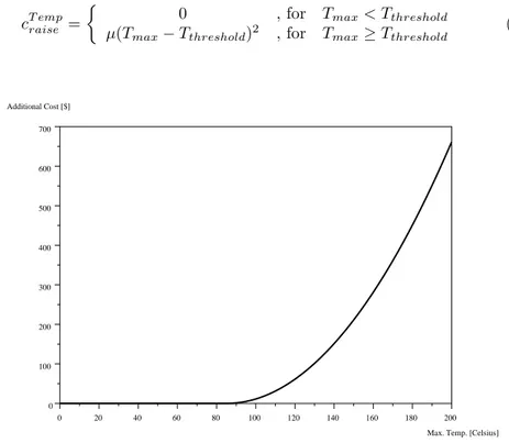
be responsible for taking into account the costs associated with maximum tem-peratures beyond the design established threshold, comprehending additional maintenance, cooling and environmental costs, for instance. In this case, we choose to use the following function to play this role:
cT empraise =
0 , for Tmax< Tthreshold
µ(Tmax−Tthreshold)2 , for Tmax≥Tthreshold (3.5)
0 20 40 60 80 100 120 140 160 180 200
0 100 200 300 400 500 600 700
Max. Temp. [Celsius] Additional Cost [$]
Figure 3.2: The penalty overheating cost function, for a threshold temperature of 85 Celsius.
WherecT empraise is the cost [$] associated with temperature raisingTmaxbeyond
the thresholdTthreshold, andµis an estimative of additional cost unit per Celsius
degree [$/oC2] (see Figure (3.2)). Unfortunately, even constructing (3.5) as a convex function of Tmax, we remark that Tmax is not smooth or continuous,
We can conceive now a performance guarantee heuristic to determine good solutions for the both point of views: thermal performance and placement cost. On the search for the optimal placement, we can examine the thermal cost component for each assignment solution, keeping the best upper bound. When the optimal placement solution is found, we just choose the lowest total cost (the best upper bound), combining placement and thermal cost components.
Defining the combined thermal-placement problem lower bound as the opti-mal solution forQAP,
LB = QAPoptimal (3.6)
and the combined thermal-placement problem upper bound as the optimal so-lution forQAP plus the associated overheating penalty,
U B = QAPoptimal + cT empraise (3.7)
we can then pick the best feasible solution found
BEST = (QAP + cT empraise)best. (3.8)
At this point we remark that the performance guarantee of a heuristic algo-rithm for a minimization problem isα(α≥1) if the algorithm is guaranteed to deliver a solutionϕwhose value is at mostαtimes the optimal value: ϕ≤αϕ∗.
Since we do not have the value of the global minimum for the combined thermal-placement problem (ϕ∗), we can only provide the following indirect relation:
LB≤ϕ∗,BEST ≤αLB,BEST ≤αϕ∗ whereα=U B/LB.
This is true because cT empraise ≥0 by construction, and it is now possible to define the optimality gap as:
GAP = BEST−LB
LB . (3.9)
An illustration of this method is depicted in Figure (3.3).
3.3
Computational Experiments
3.3.1
Experiment Description
80 82 84 86 88 90 92 94 96 98 100 102 104 106 108 110 112 114 116 118 120 122 124 126 128 130 132 134 136 138
0 10 20 30 40 50 60 70 80 90 100
Benders iterations h
C o s t [ $ ]
Placement Cost ($)
Total Cost ($) (Placement + Thermal)
Optimal Placement
Solution Best Feasible
Solution
Figure 3.3: Evolution of bounds during the method execution.
In this context, we have chosen to establish linear installation costs p = (P
(k,i)aki) varying from near 1 to 4 times the magnitude of the quadratic
cost component q = (P (i,j)
P
(k,l)cijfijkl). These linear costs were generated
randomly with the aid of the standard pseudo-random number generator imple-mented on the GNU C compiler GCC version 3.0. In fact, the addition of the linear installation costs was directly responsible for the efficiency of the solution procedure when dealing with larger instances, since this increases the master problem strength.