HESSD
12, 6831–6879, 2015Stochastic precipitation nowcasting in
Belgium
L. Foresti et al.
Title Page
Abstract Introduction
Conclusions References
Tables Figures
◭ ◮
◭ ◮
Back Close
Full Screen / Esc
Printer-friendly Version Interactive Discussion
Discussion
P
a
per
|
Discussion
P
a
per
|
Discussion
P
a
per
|
Discussion
P
a
per
|
Hydrol. Earth Syst. Sci. Discuss., 12, 6831–6879, 2015 www.hydrol-earth-syst-sci-discuss.net/12/6831/2015/ doi:10.5194/hessd-12-6831-2015
© Author(s) 2015. CC Attribution 3.0 License.
This discussion paper is/has been under review for the journal Hydrology and Earth System Sciences (HESS). Please refer to the corresponding final paper in HESS if available.
Development and verification of
a real-time stochastic precipitation
nowcasting system for urban hydrology
in Belgium
L. Foresti1, M. Reyniers1, A. Seed2, and L. Delobbe1
1
Royal Meteorological Institute of Belgium, Brussels, Belgium
2
Bureau of Meteorology, Centre for Australian Weather and Climate Research, Melbourne, Australia
Received: 26 May 2015 – Accepted: 16 June 2015 – Published: 20 July 2015
Correspondence to: L. Foresti ([email protected])
HESSD
12, 6831–6879, 2015Stochastic precipitation nowcasting in
Belgium
L. Foresti et al.
Title Page
Abstract Introduction
Conclusions References
Tables Figures
◭ ◮
◭ ◮
Back Close
Full Screen / Esc
Printer-friendly Version Interactive Discussion
Discussion
P
a
per
|
Discussion
P
a
per
|
Discussion
P
a
per
|
Discussion
P
a
per
Abstract
The Short-Term Ensemble Prediction System (STEPS) is implemented in real-time at the Royal Meteorological Institute (RMI) of Belgium. The main idea behind STEPS is to quantify the forecast uncertainty by adding stochastic perturbations to the deterministic Lagrangian extrapolation of radar images. The stochastic perturbations
5
are designed to account for the unpredictable precipitation growth and decay processes and to reproduce the dynamic scaling of precipitation fields, i.e. the observation that large scale rainfall structures are more persistent and predictable than small scale convective cells. This paper presents the development, adaptation and verification of the system STEPS for Belgium (STEPS-BE). STEPS-BE provides in real-time 20
10
member ensemble precipitation nowcasts at 1 km and 5 min resolution up to 2 h lead time using a 4 C-band radar composite as input. In the context of the PLURISK project, STEPS forecasts were generated to be used as input in sewer system hydraulic models for nowcasting urban inundations in the cities of Ghent and Leuven. Comprehensive forecast verification was performed in order to detect systematic biases over the given
15
urban areas and to analyze the reliability of probabilistic forecasts for a set of case studies in 2013 and 2014. The forecast biases over the cities of Leuven and Ghent were found to be small, which is encouraging for future integration of STEPS nowcasts into the hydraulic models. Probabilistic forecasts of exceeding 0.5 mm h−1 are reliable up to 60–90 min lead time, while the ones of exceeding 5.0 mm h−1 are only reliable
20
up to 30 min. The STEPS ensembles are slightly under-dispersive and represent only 80–90 % of the forecast errors.
1 Introduction
The use of radar measurements for urban hydrological applications has substantially increased during the last years (e.g. Berne et al., 2004; Einfalt et al., 2004; Bruni et al.,
25
radar-HESSD
12, 6831–6879, 2015Stochastic precipitation nowcasting in
Belgium
L. Foresti et al.
Title Page
Abstract Introduction
Conclusions References
Tables Figures
◭ ◮
◭ ◮
Back Close
Full Screen / Esc
Printer-friendly Version Interactive Discussion
Discussion
P
a
per
|
Discussion
P
a
per
|
Discussion
P
a
per
|
Discussion
P
a
per
|
based very short-term precipitation forecasting (nowcasting) has potential to extend the lead time of hydrological and hydraulic flow predictions.
Quantitative precipitation nowcasting (QPN) is traditionally done by estimating the apparent movement of radar precipitation fields using optical flow or variational echo tracking techniques and extrapolating the last observed precipitation field into the future
5
(e.g. Germann and Zawadzki, 2002; Bowler et al., 2004a).
Due to the lack of predictability of rainfall growth and decay processes at small spatial scales (Radhakrishna et al., 2012), it is very important to provide together with a forecast an estimation of its uncertainty. The established method to represent the forecast uncertainty in Numerical Weather Prediction (NWP) is to generate an
10
ensemble of forecasts by perturbing the initial conditions of the model in the directions exhibiting the largest error growth, which amplify more the spread of the obtained ensemble. However, in the nowcasting range the computation of large NWP ensembles (50–100 members) that resolve features at the scales of 1 km and are updated every 5 min is still impossible to achieve. Consequently, the efforts in nowcasting research
15
have recently focused on developing heuristic techniques for probabilistic precipitation nowcasting, which was the topic of the Heuristic Probabilistic Forecasting Workshop that was organized in Munich, Germany (Foresti et al., 2014).
Probabilistic QPN methods can be categorized into three main classes: analogue, local Lagrangian and stochastic approaches. The analogue-based approach derives
20
the forecast probability density function (p.d.f.) by retrieving a set of similar situations from an archive of precipitation events (Panziera et al., 2011; Foresti et al., 2015), the local Lagrangian approach derives the p.d.f. by collecting the precipitation values in a neighborhood of a given grid point in Lagrangian frame of reference (Hohti et al., 2000; Germann and Zawadzki, 2004) and the stochastic approach exploits a random
25
HESSD
12, 6831–6879, 2015Stochastic precipitation nowcasting in
Belgium
L. Foresti et al.
Title Page
Abstract Introduction
Conclusions References
Tables Figures
◭ ◮
◭ ◮
Back Close
Full Screen / Esc
Printer-friendly Version Interactive Discussion
Discussion
P
a
per
|
Discussion
P
a
per
|
Discussion
P
a
per
|
Discussion
P
a
per
stochastic approach is also extensively used to produce ensembles of precipitation fields that characterize the radar measurement uncertainty (e.g. Jordan et al., 2003; Germann et al., 2009) and for design storm studies (e.g. Willems, 2001a; Paschalis et al., 2013).
Uncertainty quantification is nowadays an integral part of both weather and
5
hydrological forecasting (Pappenberger and Beven, 2006). Not surprisingly, an important part of hydro-meteorological research aims at understanding how to propagate the uncertainty of precipitation observations and forecasts into the hydrological models (e.g. Willems, 2001b; Cloke and Pappenberger, 2009; Collier, 2009; Zappa et al., 2010).
10
Several studies already analyzed the value of deterministic nowcasting systems for catchment hydrology (e.g. Berenguer et al., 2005) and for better control of urban drainage systems (e.g. Achleitner et al., 2009; Verworn et al., 2009; Thorndahl and Rasmussen, 2013). Since an important fraction of the uncertainty of hydrological predictions is due to the uncertainty of the input rainfall observations and forecasts,
15
radar-based ensemble nowcasting systems are increasingly used as inputs for flood and sewer system modeling (e.g. Ehret et al., 2008; Silvestro and Rebora, 2012; Silvestro et al., 2013; Xuan et al., 2009, 2014). At longer forecast ranges, the NWP ensembles are also largely exploited for uncertainty propagation into hydrological models (see Roulin and Vannitsem, 2005; Thielen et al., 2009; Schellekens et al.,
20
2011).
The Short-Term Ensemble Prediction System (STEPS) is a probabilistic nowcasting system developed at the Australian Bureau of Meteorology and the UK MetOffice (see the series of papers Seed, 2003; Bowler et al., 2006; Seed et al., 2013). STEPS is operationally used at both weather offices and provides short-term ensemble
25
HESSD
12, 6831–6879, 2015Stochastic precipitation nowcasting in
Belgium
L. Foresti et al.
Title Page
Abstract Introduction
Conclusions References
Tables Figures
◭ ◮
◭ ◮
Back Close
Full Screen / Esc
Printer-friendly Version Interactive Discussion
Discussion
P
a
per
|
Discussion
P
a
per
|
Discussion
P
a
per
|
Discussion
P
a
per
|
The stochastic perturbations are designed to represent the scale-dependence of the predictability of precipitation and to reproduce the correct spatio-temporal correlation and growth of the forecast errors.
One of the first applications of STEPS in hydrology is presented in Pierce et al. (2005), who used the STEPS ensemble nowcasts to quantify the accuracy of flow
5
predictions in a medium-sized catchment in the UK. The value of STEPS nowcasts for urban hydrology was extensively analyzed by Liguori and Rico-Ramirez (2012, 2013), Liguori et al. (2012), Xuan et al. (2014). Liguori and Rico-Ramirez (2012) concluded that the skill of the radar-based extrapolation nowcast can be improved after 1 h lead time if blended with the output of NWP model. They also found that according to
10
the Receiver Operating Characteristic (ROC) curve the probabilistic nowcasts have more discrimination power than the deterministic ones. Liguori et al. (2012) integrated STEPS nowcasts as inputs into sewer system hydraulic models in an urban catchment in Yorkshire (UK). They concluded that the blending of radar and NWP forecasts has potential to increase the lead time of flow predictions, but is strongly limited by the
15
low accuracy of the NWP model in forecasting small scale features. Liguori and Rico-Ramirez (2013) performed a detailed verification of the accuracy of flow predictions and concluded that the STEPS ensembles provide similar skill than using a deterministic STEPS control forecast, but the ensembles lead to a slight underestimation of the flow predictions. Xuan et al. (2014) used ensemble STEPS nowcasts as input in a lumped
20
hydrological model for a medium-sized catchment in the South-West of the UK. The hydrological model calibrated with rain gauges had lower RMSE than the one using radar data, but the ability of STEPS in accounting for the forecast uncertainty was useful to capture some of the high flow peaks and extending the forecast lead time. However, the conclusions of the previous studies are strongly affected by the limited
25
HESSD
12, 6831–6879, 2015Stochastic precipitation nowcasting in
Belgium
L. Foresti et al.
Title Page
Abstract Introduction
Conclusions References
Tables Figures
◭ ◮
◭ ◮
Back Close
Full Screen / Esc
Printer-friendly Version Interactive Discussion
Discussion
P
a
per
|
Discussion
P
a
per
|
Discussion
P
a
per
|
Discussion
P
a
per
The goal of this paper is to present the development and verification of the STEPS system at the Royal Meteorological Institute of Belgium (RMI), referred to as STEPS-BE. STEPS-BE provides in real-time 20 member ensemble precipitation nowcasts at 1 km and 5 min resolutions up to 2 h lead time on a 512×512 domain using the Belgian 4 C-band radar composite as input. It was developed in the framework of the
5
Belspo project PLURISK for better management of rainfall-induced risks in the urban environment. Ensemble STEPS nowcasts are computed for a set of sewer overflow cases that affected the cities of Leuven and Ghent in 2013 and 2014. The accuracy of the ensemble mean forecast is verified using both continuous verification scores (multiplicative bias, RMSE) and categorical scores derived from the contingency table
10
(probability of detection, false alarm ratio and Gilbert skill score). However, the most interesting contribution of this paper is the probabilistic and ensemble verification of STEPS nowcasts using both stratiform and convective rainfall events. Probabilistic nowcasts are verified using reliability diagrams and ROC curves. On the other hand, the dispersion of the nowcast ensembles is verified using rank histograms and by
15
comparing the ensemble spread to the error of the ensemble mean.
The paper is structured as follows. Section 2 presents the radar data processing and case studies that are used to generate and verify the STEPS forecasts. Section 3 describes the nowcasting system STEPS, its extension and local implementation for Belgium (STEPS-BE). Section 4 illustrates the forecast verification results. Section 5
20
concludes the paper and discusses future perspectives.
2 Radar data and precipitation case studies
STEPS-BE integrates as input a composite image produced from the C-band radars of Wideumont (RMI, single-pol), Zaventem (Belgocontrol, single-pol), Jabbeke (RMI, dual-pol) and Avesnois (Météo-France, dual-dual-pol). The composite is produced on a 500 m
25
HESSD
12, 6831–6879, 2015Stochastic precipitation nowcasting in
Belgium
L. Foresti et al.
Title Page
Abstract Introduction
Conclusions References
Tables Figures
◭ ◮
◭ ◮
Back Close
Full Screen / Esc
Printer-friendly Version Interactive Discussion
Discussion
P
a
per
|
Discussion
P
a
per
|
Discussion
P
a
per
|
Discussion
P
a
per
|
Indicator (CAPPI) products. The compositing algorithm takes the maximum reflectivity value from each radar at each grid point.
The radars have different hardware, scanning strategies and are operated by different agencies (RMI, Belgocontrol and MétéoFrance), which inevitably leads to differences in the data processing. The Wideumont and Zaventem radars eliminate
5
the non-meteorological echoes using standard Doppler filtering. The Jabbeke radar includes an additional clutter filtering which uses a fuzzy logic algorithm based on the dual-polarization moments (essentially the co-polar correlation coefficient, the texture of the differential reflectivity and the texture of the specific differential phase shift). A static ground clutter map and a statistical filter are used by Météo-France to
10
remove the non-meteorological echoes of the Avensois radar. The French radar data processing chain is described in Tabary (2007) and in Figueras i Ventura and Tabary (2013).
Since the Zaventem radar is mainly used for aviation applications, its scanning strategy is optimized for the measurement of winds. Except for the lowest elevation
15
scan, a dual PRF mode (1200/800 Hz) is used. The azimuths that are scanned with a high PRF (1200 Hz) only have a maximum range of 125 km and are more affected by the second trip echoes caused by convective cells located beyond the 125 km range. All radars use the standard Marshall–Palmer relationshipZ=200R1.6 to convert the measured reflectivity to rainfall rate.
20
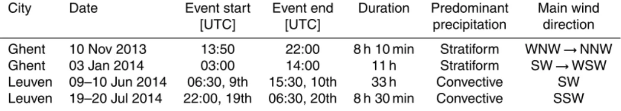
STEPS forecasts were generated and verified for a set of sewer system overflow cases that affected the cities of Ghent and Leuven (see Table 1). The Ghent cases have a more stratiform character and occurred in late autumn and winter. On the other hand, the Leuven cases are more convective and occurred in summer months. A detailed climatology of convective storms in Belgium can be found in Goudenhoofdt
25
HESSD
12, 6831–6879, 2015Stochastic precipitation nowcasting in
Belgium
L. Foresti et al.
Title Page
Abstract Introduction
Conclusions References
Tables Figures
◭ ◮
◭ ◮
Back Close
Full Screen / Esc
Printer-friendly Version Interactive Discussion
Discussion
P
a
per
|
Discussion
P
a
per
|
Discussion
P
a
per
|
Discussion
P
a
per
3 Short-Term Ensemble Prediction System (STEPS)
3.1 STEPS description
The Short-Term Ensemble Prediction System (STEPS) was jointly developed by the Australian Bureau of Meteorology (BOM) and the UK MetOffice (Bowler et al., 2006). STEPS forecasts are produced operationally at both weather services and are
5
distributed to weather forecasters and a number of external users, in particular the hydrological services.
The key idea behind STEPS is to account for the unpredictable rainfall growth and decay processes by adding stochastic perturbations to the deterministic extrapolation of radar images (Seed, 2003). In order to be effective, the stochastic perturbations
10
need to reproduce important statistical properties of both the precipitation fields and the forecast errors:
1. Spatial scaling of precipitation fields,
2. Dynamic scaling of precipitation fields,
3. Spatial correlation of the forecast errors,
15
4. Temporal correlation of the forecast errors.
The spatial scaling considers the precipitation field as arising from multiplicative cascade processes (Schertzer and Lovejoy, 1987; Seed, 2003). The presence of spatial scaling can be demonstrated by computing the 2-D Fourier power spectrum (PS) of the precipitation field. A 1-D PS can be obtained by radially averaging the
20
2-D PS. The precipitation field is said to be scaling if the 1-D PS draws a straight line on the log-log plot of the power against the spatial frequency (power law), which can be parametrized by a one or two spectral exponents (see e.g. Seed et al., 2013; Foresti and Seed, 2014). Within the multiplicative framework, a rainfall field is not represented as a collection of convective cells of a characteristic size but rather as
HESSD
12, 6831–6879, 2015Stochastic precipitation nowcasting in
Belgium
L. Foresti et al.
Title Page
Abstract Introduction
Conclusions References
Tables Figures
◭ ◮
◭ ◮
Back Close
Full Screen / Esc
Printer-friendly Version Interactive Discussion
Discussion
P
a
per
|
Discussion
P
a
per
|
Discussion
P
a
per
|
Discussion
P
a
per
|
a hierarchy of precipitation structures embedded in each other over a continuum of scales. STEPS considers the spatial scaling by decomposing the radar rainfall field into a multiplicative cascade using a fast Fourier transform (FFT) to isolate a set of 8 spatial frequencies (Seed, 2003; Bowler et al., 2006; Seed et al., 2013). Another important behavior of rainfall fields is known asdynamic scaling, which is the empirical
5
observation that the rate of temporal development of rainfall structures is a power law function of their spatial scale (Venugopal et al., 1999; Foresti and Seed, 2014). This means that large precipitation features are more persistent and predictable compared with small precipitation cells, which is closely related to concept of scale-dependence of the predictability of precipitation (Germann and Zawadzki, 2002; Turner et al., 2004).
10
The stochastic perturbations should be able to reflect the properties of the forecast errors. Generating spatially and temporally correlated forecast errors is mandatory for hydrological applications, in particular when the correlation length of the errors is comparable or superior to the size and response time of the catchment.Spatially correlated stochastic noisecan be constructed by power law filtering a white noise field
15
(Schertzer and Lovejoy, 1987). In practice it consists of three steps: computing the FFT of a white noise field, multiplying the obtained components in frequency domain by a given filter and applying the inverse FFT to return back to the spatial domain. The 1-D or 2-D power spectra of the rainfall field can be used as filter to obtain noise fields that have the same scaling and spatial correlation of the rainfall field. The 1-D PS of
20
the precipitation fields often appears to be a power law of the spatial frequency and explains why the procedure is also called power law filtering of white noise. In order to represent the anisotropies of the precipitation field the 2-D PS can also be used as filter. In the absence of a target precipitation field from which to derive the PS, the filter can be parametrized by using a climatological power law (see Seed et al., 2013).
25
HESSD
12, 6831–6879, 2015Stochastic precipitation nowcasting in
Belgium
L. Foresti et al.
Title Page
Abstract Introduction
Conclusions References
Tables Figures
◭ ◮
◭ ◮
Back Close
Full Screen / Esc
Printer-friendly Version Interactive Discussion
Discussion
P
a
per
|
Discussion
P
a
per
|
Discussion
P
a
per
|
Discussion
P
a
per
The practical implementation of STEPS to reproduce these important properties consists of the following steps (see Bowler et al., 2006; Foresti and Seed, 2014):
1. Estimation of the velocity field using optical flow on the last two radar rainfall images (Bowler et al., 2004a).
2. Decomposition of both rainfall fields into a multiplicative cascade using an FFT to
5
isolate a set of 8 spatial frequencies.
3. Estimation of the rate of temporal evolution of rainfall features at each level of the cascade (Lagrangian auto-correlation).
4. Generation of a cascade of spatially correlated stochastic noise using as filter the 1-D or 2-D power spectra of the last radar rainfall field.
10
5. Stochastic perturbation of the rainfall cascade using the noise cascade (level by level).
6. Extrapolation of the cascade levels using a semi-Lagrangian advection scheme.
7. Application of the AR(1) or AR(2) model for the temporal update of the cascade levels at each forecast lead time using the Lagrangian auto-correlations estimated
15
in step (3).
8. Recomposition of the cascade into a rainfall field.
9. Probability matching of the forecast rainfall field with the original observed field (Ebert, 2001).
10. Computation of the forecast rainfall accumulations from the instant forecast rainfall
20
HESSD
12, 6831–6879, 2015Stochastic precipitation nowcasting in
Belgium
L. Foresti et al.
Title Page
Abstract Introduction
Conclusions References
Tables Figures
◭ ◮
◭ ◮
Back Close
Full Screen / Esc
Printer-friendly Version Interactive Discussion
Discussion
P
a
per
|
Discussion
P
a
per
|
Discussion
P
a
per
|
Discussion
P
a
per
|
3.2 STEPS implementation at RMI (STEPS-BE)
Bowler et al. (2006) introduced a general framework for blending a radar-based extrapolation nowcast with one or more outputs of downscaled NWP models. Because of being designed for urban applications, the maximum lead time of STEPS-BE forecasts is restricted to 2 h. The operational NWP model of RMI (ALARO) runs only 4
5
times daily using a grid spacing of 4 km. Considering the model spin-up time and the absence of radar data assimilation, it is very unlikely that ALARO provides useful skill for blending its output with a radar-based extrapolation nowcast within the considered nowcasting range. It must also be reminded that the effective resolution of NWP models is much larger than the grid spacing. For instance, Grasso (2000) estimates
10
the effective resolution to be at least 4 times the grid spacing, while Skamarock (2004) estimates it to be up to 7 times the grid spacing. ALARO would then only be able to resolve features that are greater than 20 km. For all these reasons, STEPS-BE only involves an extrapolation nowcast without NWP blending.
The STEPS-BE forecast domain is smaller than the extent of the 4 C-band radars
15
composite (see Fig. 1). The radar field was upscaled from the original resolution of 500 m to 1 km and a sub-region of 512×512 grid points centered over Belgium was extracted.
STEPS-BE includes a couple of improvements compared with the original implementation of the BOM:
20
1. Kernel interpolation of optical flow vectors,
2. Generation of stochastic noise only within the advected radar mask.
The optical flow algorithm of Bowler et al. (2004a) estimates the velocity field by dividing the radar domain into a series of blocks within which the optical flow equation is solved. The minimization of the field divergence is only performed at the level of the
25
HESSD
12, 6831–6879, 2015Stochastic precipitation nowcasting in
Belgium
L. Foresti et al.
Title Page
Abstract Introduction
Conclusions References
Tables Figures
◭ ◮
◭ ◮
Back Close
Full Screen / Esc
Printer-friendly Version Interactive Discussion
Discussion
P
a
per
|
Discussion
P
a
per
|
Discussion
P
a
per
|
Discussion
P
a
per
the velocity vectors located at the center of the blocks onto the fine radar grid. The bandwidth of the Gaussian kernel was chosen to beσ=24 km=0.4k, where k=60 grid points is the block size. This setting has the advantage of obtaining velocity fields that are less affected by the differential motion of small rainfall features and the presence of ground clutter. A too precise velocity field would provide increased
5
predictability at very-short lead times but worse forecasts at longer lead times due to excessive convergence and divergence of precipitation features during the advection. Smooth velocity fields could also be obtained by using a smaller block size and compensating with a larger bandwidth of the smoothing kernel.
In STEPS-BE the 1-D power spectrum of the last rainfall field is used as filter
10
to generate the spatially correlated stochastic perturbations. If the rainfall fraction is inferior to 3 %, the PS is parameterized using two spectral slopes to account for a scaling break that is often observed at the wavelength of 40 km (see Seed et al., 2013; Foresti and Seed, 2014). To simplify the computations, an auto-regressive model of order 1 (AR(1)) was employed for imposing the temporal correlations and to model
15
the growth of forecast errors.
Since STEPS-BE does not blend the extrapolation nowcast with the output of NWP, there is as side effect the appearance of small amounts of stochastic rain also outside of the non-rectangular domain covered by the radars. This feature becomes an issue when advecting the radar mask over several time steps. Large areas with small
20
amounts of stochastic rain appear outside of the validity domain of the forecast and perturb the probability matching. In STEPS-BE the stochastic perturbations are only generated within the advected radar domain and set to zero elsewhere.
STEPS-BE can also account for the uncertainty due to the future evolution of the diagnosed velocity field. The STEPS version that is implemented in the UK (Bowler
25
HESSD
12, 6831–6879, 2015Stochastic precipitation nowcasting in
Belgium
L. Foresti et al.
Title Page
Abstract Introduction
Conclusions References
Tables Figures
◭ ◮
◭ ◮
Back Close
Full Screen / Esc
Printer-friendly Version Interactive Discussion
Discussion
P
a
per
|
Discussion
P
a
per
|
Discussion
P
a
per
|
Discussion
P
a
per
|
field is multiplied by a single factorCthat is drawn from the following distribution:
C=101.5N/10, (1)
whereN is a normally distributed random variable with zero mean and unit variance. In other words, the velocity field is accelerated or decelerated by a single random factor without affecting the direction of the vectors. In fact, the uncertainty on the diagnosed
5
speed was observed to be higher than the one of the direction of movement (Bowler et al., 2006).
The BOM and RMI versions of STEPS also include a stochastic model for the radar measurement error, a broken-line model to account for the unknown future evolution of the mean areal rainfall and the possibility to use time-lagged ensembles. However,
10
a nowcasting model with too many components is harder to calibrate and complicates the interpretation of the forecast fields. Because of these reasons, STEPS-BE only exploits the basic stochastic model of the evolution of velocity and rainfall fields (due to growth and decay processes).
The core of STEPS-BE is implemented in C/C++ and the production of figures
15
in python. Bash scripts were written to call multiple STEPS instances and compute the ensemble members in parallel over several processors. Once all the ensemble members are computed, a separate script collects the corresponding netCDF files and calculates the forecast probabilities. Most of the computational cost of STEPS consists of filtering the white noise field with FFT, advecting and updating the radar cascade
20
with the AR model. The re-calculation of optical flow fields on each processor takes less than 10 % of the total computational time. Thus, a parallel re-design of the STEPS source code was not needed (e.g. using openMP or MPI implementations).
The python matplotlib library is used to read the netCDF files, export the PNG figures and the time series of observed and forecast rainfall at the location of major cities
25
HESSD
12, 6831–6879, 2015Stochastic precipitation nowcasting in
Belgium
L. Foresti et al.
Title Page
Abstract Introduction
Conclusions References
Tables Figures
◭ ◮
◭ ◮
Back Close
Full Screen / Esc
Printer-friendly Version Interactive Discussion
Discussion
P
a
per
|
Discussion
P
a
per
|
Discussion
P
a
per
|
Discussion
P
a
per
composites and triggers STEPS-BE once a field with a new time stamp is found. All these implementation details ensure that the user/forecaster can have access to an ensemble STEPS nowcast in less than 5 min after receiving the radar composite image.
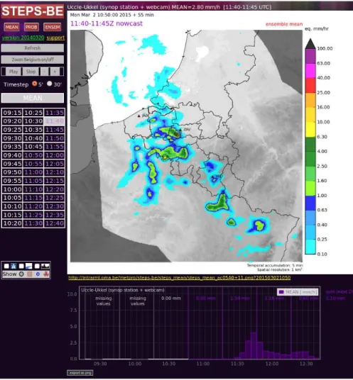
The visualization system of STEPS-BE is very similar to the one of INCA-BE, the
5
local Belgian implementation of the Integrated Nowcasting through Comprehensive Analysis system (INCA, Haiden et al., 2011) developed at the Austrian weather office (ZAMG). Figure 1 illustrates the web interface with an example of an ensemble mean nowcast. The user can highlight the major cities, weather stations and click to visualize the time series of observed and forecast precipitation/probability, which appears at
10
the bottom of the web page. The navigation through the observations and forecast lead times is facilitated by the scroll wheel of the mouse. On the other hand, by clicking on the image it is possible to easily scroll through the various ensemble members or probability levels. Scrolling the ensemble members at different lead times is very instructive and can make the user aware of the forecast uncertainty. In fact,
15
at a lead time of 5 min the ensemble members agree very well on the intensity and location of precipitation. This means that the ensemble spread is small and the probabilistic forecast is sharp, i.e. most of the forecast probabilities are close to 1 or 0 (see explanation in Appendix A). On the other hand, at 1 or 2 h lead time the ensemble members disagree on the location and intensity of rainfall, which enhances
20
the ensemble spread and decreases the sharpness of the probabilistic forecast. The web page includes extensive documentation to guide the user and a set of case studies to help understanding the strengths and limitations of STEPS. The visualization system was implemented with great attention to take full advantage of the multi-dimensional information content of probabilistic and ensemble forecasts.
HESSD
12, 6831–6879, 2015Stochastic precipitation nowcasting in
Belgium
L. Foresti et al.
Title Page
Abstract Introduction
Conclusions References
Tables Figures
◭ ◮
◭ ◮
Back Close
Full Screen / Esc
Printer-friendly Version Interactive Discussion
Discussion
P
a
per
|
Discussion
P
a
per
|
Discussion
P
a
per
|
Discussion
P
a
per
|
4 Forecast verification
4.1 Verification set-up
This section presents the verification of STEPS-BE forecasts using a set of case studies (see Sect. 2). The accumulated radar observations were employed as reference for the verification. The rainfall rates are accumulated over the last 5 min
5
by reversing the velocity field vectors and performing the advection correction. The verification procedure follows the one presented in Foresti and Seed (2015), which was designed to analyze the spatial distribution of the forecast errors. The 30 min ensemble mean forecast was verified against the observed 30 min radar accumulations using both continuous and categorical verification scores. The continuous scores include
10
the multiplicative bias and the root mean squared error (RMSE), while the categorical scores include the probability of detection (POD), false alarm ratio (FAR) and Gilbert skill score (GSS) derived from the contingency table for rainfall thresholds of 0.5 and 5.0 mm h−1. The rainfall thresholds are given in equivalent intensity independently of the forecast rainfall accumulation. Thus, a threshold of 5.0 mm h−1 on a 30 min
15
accumulation corresponds to 2.5 mm of rain. The multiplicative bias and the RMSE were evaluated only at the locations where the forecast or the verifying observations exceeded 0.1 mm h−1, which can be referred to as aweakly conditional verification. The probabilistic forecast of exceeding 0.1, 0.5, 5.0 mm h−1was verified using the reliability diagrams and ROC curves. Finally, the dispersion of the ensemble was analyzed by
20
comparing the ensemble spread to the RMSE of the ensemble mean and by using rank histograms. More details about the forecast verification setup and scores are given in Appendix A.
4.2 Deterministic verification
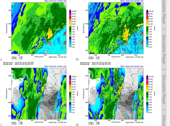
Figures 2 and 3 show the mean forecast and observed rainfall rates corresponding
25
HESSD
12, 6831–6879, 2015Stochastic precipitation nowcasting in
Belgium
L. Foresti et al.
Title Page
Abstract Introduction
Conclusions References
Tables Figures
◭ ◮
◭ ◮
Back Close
Full Screen / Esc
Printer-friendly Version Interactive Discussion
Discussion
P
a
per
|
Discussion
P
a
per
|
Discussion
P
a
per
|
Discussion
P
a
per
The mean was computed using the weak conditional principle explained above. The average forecast and observed accumulations generally agree very well for the 0– 30 min lead time forecast. The Leuven case on 10 November 2013 (Fig. 2a and b) is the only one with northwesterly flows and is characterized by the lowest average rainfall rates. The Avesnois radar demonstrates very well the range-dependence of
5
the average rainfall rates, which gradually decrease with increasing distance from the radar. On the contrary, the smaller ring of high rainfall rates around the Zaventem radar is mostly due to the bright band (Fig. 2b). The Ghent case on 03 January 2014 has higher rainfall rates and the elongated structures of precipitation areas demonstrate well the southwesterly flow regime (Fig. 2c and d). For this case the measurements
10
of the Zaventem radar are also affected by second trip echoes, which appear as a set of alternating rainfall features North-West of the radar. These alternating patterns are explained by the dual PRF mode of Zaventem (see Sect. 2). The Leuven cases on 9 June 2014 and 19–20 July 2014 have an important convective activity (Fig. 3a–d). The maximum average rainfall rates are located over the Ardennes mountain range and
15
the city of Leuven respectively. Since urban flash floods can be triggered by a single convective cell, the average rainfall rate over the duration of the event may not be as high in the considered city (e.g. Fig. 3b).
Figure 4 illustrates the multiplicative bias of the 0–30 min nowcast averaged over each of the 4 events. A detailed interpretation of such forecast biases using Australian
20
radar data and their connection to orographic features is given in Foresti and Seed (2015), which point out that an important fraction of forecast errors is caused by the biases of the verifying radar observations rather than systematic rainfall growth and decay processes due to orography. In Fig. 4a it is easy to notice the effect of bright band, which causes a series of systematic forecast biases around the Zaventem
25
HESSD
12, 6831–6879, 2015Stochastic precipitation nowcasting in
Belgium
L. Foresti et al.
Title Page
Abstract Introduction
Conclusions References
Tables Figures
◭ ◮
◭ ◮
Back Close
Full Screen / Esc
Printer-friendly Version Interactive Discussion
Discussion
P
a
per
|
Discussion
P
a
per
|
Discussion
P
a
per
|
Discussion
P
a
per
|
and therefore strongly underestimated by STEPS. The only situation where the range dependence of the rainfall estimation does not affect the forecast verification occurs when the velocity field is perfectly rotational and centered on the radar (assuming no beam blockage). All the other cases have to deal with the fact that the rainfall nowcast also extrapolates the biases of the radar observations! Contrarily to the
5
expectations, on the upwind side of the Ardennes there is overestimation, which may depict a region of systematic rainfall decay. The bias over the city of Ghent is fortunately small and is comprised between 0 and +0.5 dB (light overestimation, rainfall decay). Having small systematic biases over the cities of interest is very important for future integration of STEPS nowcasts as input in hydraulic models. In Fig. 4b the systematic
10
underestimation is also located upstream with respect to the prevailing winds (SW). Also in this case the bias over the city of Ghent is small but comprised between −0.5 and 0 dB (light underestimation, rainfall growth). The strong overestimations in Germany and The Netherlands are mostly due to the underestimation of rainfall by the verifying radar observations rather than caused by systematic rainfall decay.
15
This is particularly visible after a range of 125 km from the Zaventem radar, which demonstrates again that discontinuities and biases in the radar observations lead to biases in the extrapolation forecast. A similar feature is visible in Fig. 4c but this time located at a range of 240 km North of the Wideumont radar when entering the area covered by the Jabbeke radar. This forecast bias is mainly explained by the negative
20
calibration bias of the Jabbeke radar, which is known to slightly underestimate the rainfall rates with respect to the Wideumont radar. Strong underestimation occurs over the Ardennes due to the systematic initiation and growth of convection that cannot be predicted by STEPS. Fortunately the city of Leuven is located in a region with small biases comprised between−0.5 and+0.5 dB. Figure 4d is quite interesting since strong
25
HESSD
12, 6831–6879, 2015Stochastic precipitation nowcasting in
Belgium
L. Foresti et al.
Title Page
Abstract Introduction
Conclusions References
Tables Figures
◭ ◮
◭ ◮
Back Close
Full Screen / Esc
Printer-friendly Version Interactive Discussion
Discussion
P
a
per
|
Discussion
P
a
per
|
Discussion
P
a
per
|
Discussion
P
a
per
which tends to drag at the rear of the rain band. The two bands of underestimations South of Leuven are caused by two different thunderstorms. The first one passed over the city of Leuven and had a stronger westerly component with respect to the prevailing southerly flow. The second thunderstorm was weaker and had a stronger easterly component. When isolated convection does not follow the prevailing movement of the
5
rainfall field, strong biases can appear in the nowcast during the first lead times. Figure 5 shows the spatial distribution of the RMSE for the stratiform event on 03 January 2014 in Ghent and the convective event on 20 July 2014 in Leuven. If compared with Figs. 2d and 3d it is clear that the RMSE is strongly correlated with the regions having the highest mean rainfall accumulations (proportional effect). Thus, it is
10
not surprising that the RMSE of the convective case (Fig. 5b) displays values exceeding 10 mm h−1 over the city of Leuven. The winter case only shows RMSE values below 2 mm h−1over the city of Ghent.
Figure 6 illustrates an example of categorical verification of the 30–60 min ensemble mean forecast for the Leuven case on 19–20 July 2014 relative to the rainfall
15
threshold of 0.5 mm h−1. The probability of detection is high everywhere (mean of 0.75) except in the neighborhood of Antwerp and South of Leuven, where the initiation of thunderstorms could not be predicted by STEPS (Fig. 6a). The false alarm ratio is quite low (mean of 0.36) and the regions with high values are mainly located at the rear of the front where the rainfall is advected too slowly compared with the actual
20
movement of the front (Fig. 6b). A high Gilbert skill score generally coincides with the regions with the highest rainfall accumulations and becomes lower at the edges of the rain areas (Fig. 6c). This finding can be explained conceptually if one thinks about the verification of the future path of a single convective cell. The regions with the highest uncertainty are located along the edges of the predicted thunderstorm path and the
25
HESSD
12, 6831–6879, 2015Stochastic precipitation nowcasting in
Belgium
L. Foresti et al.
Title Page
Abstract Introduction
Conclusions References
Tables Figures
◭ ◮
◭ ◮
Back Close
Full Screen / Esc
Printer-friendly Version Interactive Discussion
Discussion
P
a
per
|
Discussion
P
a
per
|
Discussion
P
a
per
|
Discussion
P
a
per
|
4.3 Probabilistic verification
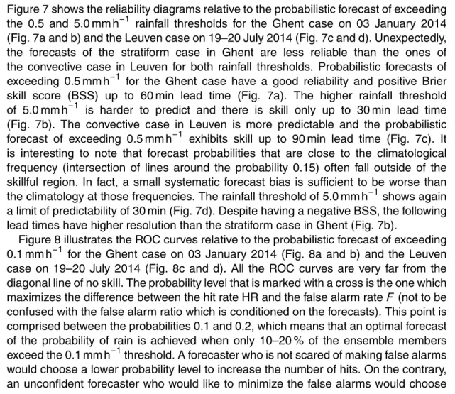
Figure 7 shows the reliability diagrams relative to the probabilistic forecast of exceeding the 0.5 and 5.0 mm h−1 rainfall thresholds for the Ghent case on 03 January 2014 (Fig. 7a and b) and the Leuven case on 19–20 July 2014 (Fig. 7c and d). Unexpectedly, the forecasts of the stratiform case in Ghent are less reliable than the ones of
5
the convective case in Leuven for both rainfall thresholds. Probabilistic forecasts of exceeding 0.5 mm h−1 for the Ghent case have a good reliability and positive Brier skill score (BSS) up to 60 min lead time (Fig. 7a). The higher rainfall threshold of 5.0 mm h−1 is harder to predict and there is skill only up to 30 min lead time (Fig. 7b). The convective case in Leuven is more predictable and the probabilistic
10
forecast of exceeding 0.5 mm h−1 exhibits skill up to 90 min lead time (Fig. 7c). It is interesting to note that forecast probabilities that are close to the climatological frequency (intersection of lines around the probability 0.15) often fall outside of the skillful region. In fact, a small systematic forecast bias is sufficient to be worse than the climatology at those frequencies. The rainfall threshold of 5.0 mm h−1 shows again
15
a limit of predictability of 30 min (Fig. 7d). Despite having a negative BSS, the following lead times have higher resolution than the stratiform case in Ghent (Fig. 7b).
Figure 8 illustrates the ROC curves relative to the probabilistic forecast of exceeding 0.1 mm h−1 for the Ghent case on 03 January 2014 (Fig. 8a and b) and the Leuven case on 19–20 July 2014 (Fig. 8c and d). All the ROC curves are very far from the
20
diagonal line of no skill. The probability level that is marked with a cross is the one which maximizes the difference between the hit rate HR and the false alarm rateF (not to be confused with the false alarm ratio which is conditioned on the forecasts). This point is comprised between the probabilities 0.1 and 0.2, which means that an optimal forecast of the probability of rain is achieved when only 10–20 % of the ensemble members
25
HESSD
12, 6831–6879, 2015Stochastic precipitation nowcasting in
Belgium
L. Foresti et al.
Title Page
Abstract Introduction
Conclusions References
Tables Figures
◭ ◮
◭ ◮
Back Close
Full Screen / Esc
Printer-friendly Version Interactive Discussion
Discussion
P
a
per
|
Discussion
P
a
per
|
Discussion
P
a
per
|
Discussion
P
a
per
a higher probability level, which has however the consequence of reducing the number of hits. As expected, the area under the ROC curves (AUC) decreases for increasing lead times. The discrimination skill for the convective event in Leuven is slightly higher than the one of the stratiform event in Ghent, which confirms the findings on the reliability diagrams (Fig. 7). This does not mean that small scale features are easier
5
to forecast than larger scales features, which is known to be false (see Foresti and Seed, 2014). It means that the predictability of well defined and organized convective systems is higher than the one of more moderate convection with shorter lifetime, at least for the cases analyzed in this paper.
4.4 Ensemble verification
10
Figure 9 compares the error of the ensemble mean (RMSE) and the ensemble spread for the Ghent case on 03 January 2014 and the Leuven case on 19–20 July 2014 (see interpretation of ensemble spread in Appendix A). In both cases the RMSE increases up to a lead time of 50–60 min and then starts a slow decrease, which can be counter-intuitive. However, it must be reminded that the ensemble mean forecast becomes
15
smoother for increasing lead times, which reduces the double penalty error due to forecasting a thunderstorm at the wrong location. The ensemble spread also increases up to 50–60 min lead time and then slowly stabilizes. For both the Ghent and Leuven cases the ensemble spread is lower than the error of the ensemble mean at all lead times, which suggests that the ensemble forecasts are under-dispersive. The degree
20
of under-dispersion is the highest at a lead time of 5 min, with the spread values being equal to 60 % of the forecast error for the winter event in Ghent (Fig. 9a) and 70 % for the summer event in Leuven (Fig. 9b). This underestimation may be attributed to using a very smooth velocity field for the advection, which does not exploit sufficiently the very short predictability of small scale precipitation features but is optimized for
25
HESSD
12, 6831–6879, 2015Stochastic precipitation nowcasting in
Belgium
L. Foresti et al.
Title Page
Abstract Introduction
Conclusions References
Tables Figures
◭ ◮
◭ ◮
Back Close
Full Screen / Esc
Printer-friendly Version Interactive Discussion
Discussion
P
a
per
|
Discussion
P
a
per
|
Discussion
P
a
per
|
Discussion
P
a
per
|
of 5 min is higher than the one at 10 min for the winter case in Ghent (Fig. 9a). For all other lead times, the ensemble spread represents 75–90 % of the forecast error for the Ghent case (Fig. 9a) and 75–80 % for the Leuven case (Fig. 9b), which is a good result. Figure 10 illustrates the rank histograms for the Leuven case on 19–20 July 2014 for lead times of 5 and 60 min. The U-shape of the rank histogram demonstrates
5
again a certain degree of ensemble under-dispersion. In particular, all ensemble members for the 5 min lead time are inferior to the observations in ∼16 % of the cases (Fig. 10a), while for the 60 min lead time it happens in more than ∼30 % of the cases (Fig. 10b). On the other hand, the fraction of observations falling below the value of the lowest ensemble member is only 8 % for both lead times.
10
Despite the fact that STEPS is designed to reproduce the space–time variability of rainfall, it underestimates a certain fraction of the observed rainfall extremes. This underestimation augments with increasing lead time and depicts an increasing smoothness of the STEPS ensembles, which is probably due to the advection of the radar rainfall cascade (see Sect. 3, step 6). In fact, the small scale rainfall features
15
represented in the lowest cascade levels suffer more from numerical diffusion during the Lagrangian extrapolation, which is observed as a gradual loss of variability in the forecast ensembles.
4.5 Verification summary of the events
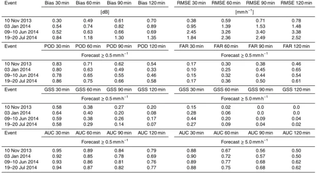
Table 2 provides a comparison of the verification scores for each event. The average
20
multiplicative biases of the 30 min lead time forecast are comprised between 0.3 and 0.8. Except for the event on 19–20 July 2014 the biases remain well below 1 dB for all lead times, which is a positive result. Of course, these are average values and locally they can even exceed 3 dB (see Fig. 4). On the other hand, the RMSE values mark more the distinction between the two winter cases in Ghent and the two summer
25
HESSD
12, 6831–6879, 2015Stochastic precipitation nowcasting in
Belgium
L. Foresti et al.
Title Page
Abstract Introduction
Conclusions References
Tables Figures
◭ ◮
◭ ◮
Back Close
Full Screen / Esc
Printer-friendly Version Interactive Discussion
Discussion
P
a
per
|
Discussion
P
a
per
|
Discussion
P
a
per
|
Discussion
P
a
per
convective cases is higher than the RMSE of a 120 min nowcast of the two stratiform cases. The probability of detection relative to the 0.5 mm h−1 threshold decreases from 78–86 to 33–58 %, while the false alarm ratio increases from 10–17 to 46–65 %. The Gilbert skill score starts with values of 0.58–0.64 and 0.29–0.40 at the 30 and 60 min lead times respectively and decays to values of 0.08–0.20 at 120 min. Wang
5
et al. (2009) reported a Critical success index value of 0.45 for STEPS nowcasts of 0–60 min accumulations relative to the 1 mm h−1threshold. Considering that the GSS is the CSI corrected by random chance, this value is comparable with the ones of the 30–60 min accumulations obtained in this paper. The GSS values relative to the threshold of 5.0 mm h−1are much lower. They oscillate between 0.15 and 0.44 for the
10
first lead time and become very low and close to 0 afterwards. Thus, the predictability of rainfall structures exceeding 5.0 mm h−1 rarely exceeds 30 min according to the GSS. The area under the ROC curve values characterizing the potential discrimination power of the probabilistic forecast of exceeding 0.5 mm h−1 start at 0.92–0.95 at 30 min lead time and decrease to 0.69–0.79 at 120 min. For the probabilistic forecast of exceeding
15
5.0 mm h−1they start at 0.88–0.90 and decrease to 0.62 for the convective cases and to 0.50 for the stratiform cases (no discrimination).
5 Conclusions
The Short-Term Ensemble Prediction System (STEPS) is a probabilistic nowcasting system based on the extrapolation of radar images developed at the Australian Bureau
20
of Meteorology in collaboration with the UK MetOffice. The principle behind STEPS is to produce an ensemble forecast by perturbing a deterministic extrapolation nowcast with stochastic noise. The perturbations are designed to reproduce the spatial and temporal correlations of the forecast errors and the scale-dependence of the predictability of precipitation.
25
HESSD
12, 6831–6879, 2015Stochastic precipitation nowcasting in
Belgium
L. Foresti et al.
Title Page
Abstract Introduction
Conclusions References
Tables Figures
◭ ◮
◭ ◮
Back Close
Full Screen / Esc
Printer-friendly Version Interactive Discussion
Discussion
P
a
per
|
Discussion
P
a
per
|
Discussion
P
a
per
|
Discussion
P
a
per
|
produces in real-time 20 member ensemble nowcasts at 1 km and 5 min resolutions up to 2 h lead time using the 4 C-band radar composite of Belgium. Compared with the original implementation, STEPS-BE includes a kernel-based interpolation of optical flow vectors to obtain smoother velocity fields and an improvement to generate stochastic noise only within the advected radar composite to respect the validity domain
5
of the nowcasts.
The performance of STEPS-BE was verified using the radar observations as reference on four case studies that caused sewer system floods in the cities of Ghent and Leuven during the years 2013 and 2014. The ensemble mean forecast of the next four 30 min accumulations was verified using the multiplicative bias, the
10
RMSE as well as some categorical scores derived from the contingency table: the probability of detection, false alarm ratio and Gilbert skill score (Equitable skill score). The spatial distribution of multiplicative biases revealed regions of systematic over-and underestimation by STEPS. The underestimations are often associated with the locations of convective initiation and thunderstorm growth, which cannot be predicted
15
by STEPS. On the other hand, the regions of overestimation are mostly due to the underestimation of rainfall by the verifying observations rather than a systematic rainfall growth (see Foresti and Seed, 2015, for a more detailed discussion). In order to disentangle the forecast and observation biases, detailed knowledge about the spatial distribution of the radar measurement errors for a given weather situation
20
is needed. The multiplicative biases over the cities of Leuven and Ghent are very low and comprised between −0.5 dB and + 0.5 dB, which is a good starting point to integrate STEPS nowcasts as input into sewer system hydraulic models. The categorical forecast verification helped discovering the places with low probability of detection due to convective initiation at the front of the rain band and high false alarm
25
HESSD
12, 6831–6879, 2015Stochastic precipitation nowcasting in
Belgium
L. Foresti et al.
Title Page
Abstract Introduction
Conclusions References
Tables Figures
◭ ◮
◭ ◮
Back Close
Full Screen / Esc
Printer-friendly Version Interactive Discussion
Discussion
P
a
per
|
Discussion
P
a
per
|
Discussion
P
a
per
|
Discussion
P
a
per
also observed that the forecasts of convective events have more skill than the ones on stratiform events. The STEPS ensembles are characterized by a certain degree of under-estimation of the forecast uncertainty, with values of the ensemble spread close to 80–90 % of the forecast error.
From a research perspective, STEPS-BE could also be extended by including
5
a stochastic model to account for the residual radar measurement errors, in particular to obtain more accurate estimations of the forecast uncertainty at short range.
Appendix: Forecast verification scores
Forecast verification is an important aspect of a forecasting system. A forecast without an estimation of its accuracy is not very informative. For an in-depth
10
description of forecast verification science and corresponding scores we refer to Jolliffe and Stephenson (2011) and the verification website maintained at the Bureau of Meteorology (http://www.cawcr.gov.au/projects/verification/).
The STEPSensemble mean forecastwas verified using the following scores:
– Multiplicative bias:
15
bias= 1
N
N
X
i=1
10log10
F
i+b
Oi+b
, (1)
where Fi is the forecast rainfall accumulation, Oi is the observed rainfall accumulation, b=2 mm h−1 is an offset to eliminate the division by zero and to reduce the contribution of the forecast errors at low rainfall intensities, and
N is the number of samples. For the specific case of the verification of the
20
HESSD
12, 6831–6879, 2015Stochastic precipitation nowcasting in
Belgium
L. Foresti et al.
Title Page
Abstract Introduction
Conclusions References
Tables Figures
◭ ◮
◭ ◮
Back Close
Full Screen / Esc
Printer-friendly Version Interactive Discussion
Discussion
P
a
per
|
Discussion
P
a
per
|
Discussion
P
a
per
|
Discussion
P
a
per
|
weak conditional verification). The bias is given in decibels [dB] in order to obtain a symmetric distribution of the multiplicative errors centered at 0, which is not possible with the simple power ratio F/O. The following table summarizes the correspondence between the decibel scale and the power ratio (Table A1).
For example, a bias of+3 dB occurs when the forecast rainfallF is twice as much
5
as the observed rainfallO.
– Root mean square error:
RMSE= v u u t1
N
N
X
i=1
(Fi−Oi)2. (2)
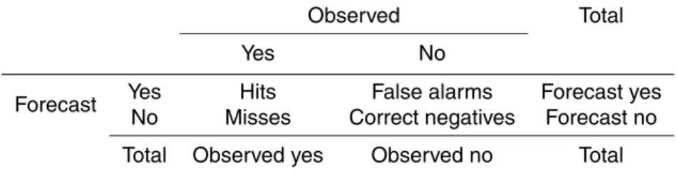
– Contingency table of a dichotomous (yes/no) forecast, see Table A2, where the hits is the number of times that both the observation and the forecast exceed
10
a given rainfall threshold (at a given grid point), thefalse alarms is the number of times that the forecast exceeds the threshold but the observation does not, the missesis the number of times that the forecast does not exceed the threshold but the observation does and thecorrect negatives is the number of times that both the observation and the forecast do not exceed the threshold.
15
– Different scores can be derived from the contingency table to characterize a particular feature or skill of the forecasting system:
– Probability of detection (hit rate):
POD= hits
hits+misses =
hits
observed yes. (3)
The POD characterizes the fraction of observed events that were correctly
20
HESSD
12, 6831–6879, 2015Stochastic precipitation nowcasting in
Belgium
L. Foresti et al.
Title Page
Abstract Introduction
Conclusions References
Tables Figures
◭ ◮
◭ ◮
Back Close
Full Screen / Esc
Printer-friendly Version Interactive Discussion
Discussion
P
a
per
|
Discussion
P
a
per
|
Discussion
P
a
per
|
Discussion
P
a
per
– False alarm ratio:
FAR= false alarms
hits+false alarms =
false alarms
forecast yes, (4)
The FAR characterizes the fraction of forecast events that were wrongly forecast.
– False alarm rate:
5
F = false alarms
false alarms+correct negatives =
false alarms
observed no. (5)
The false alarm rate F is conditioned on the observations, while the false alarm ratio FAR on the forecasts.
– Gilbert skill score (equitable threat score):
GSS= hits−hitsrandom
hits+misses+false alarms−hitsrandom
, (6)
10
where hitsrandom=
(hits+misses)(hits+false alarms) total
=(observed yes)(forecast yes)
total . (7)
is the number of hits obtained by random chance, which is calculated by multiplying the marginal sums of the observed and forecast events (such as computing the theoretical frequencies for the Chi-squared test). The
15
HESSD
12, 6831–6879, 2015Stochastic precipitation nowcasting in
Belgium
L. Foresti et al.
Title Page
Abstract Introduction
Conclusions References
Tables Figures
◭ ◮
◭ ◮
Back Close
Full Screen / Esc
Printer-friendly Version Interactive Discussion
Discussion
P
a
per
|
Discussion
P
a
per
|
Discussion
P
a
per
|
Discussion
P
a
per
|
The accuracy of probabilistic forecasts can be verified in various ways. In this paper we employ the reliability diagram and the Receiver Operating Characteristic curve (ROC). The reliability diagram compares the forecast probability with the observed frequency. Reliability characterizes the agreement between the forecast probability and observed frequency. For a reliable forecasting system the two values should be
5
the same, which happens for example when we observe rain 80 % of the time when it is forecast with 80 % probability (in average, diagonal line of Fig. 8). Unreliable forecasts exhibit departures from this optimum (bias). Resolution characterizes the ability of the forecasts to categorize the observed frequencies into distinct classes. The complete lack of resolution occurs when the forecast probabilities are completely
10
unable to distinguish the observed frequencies, which corresponds to the climatological frequency of exceeding a given rainfall threshold during that event (horizontal dashed line in Fig. 8). The Brier skill score characterizes the relative skill of the probabilistic forecast compared with the one obtained by using the climatological frequency (see Jolliffe and Stephenson, 2011). The region where the probabilistic forecast has
15
a positive Brier skill score, i.e. it is better than simply taking the climatological frequency as forecast, is grayed out (see Fig. 8). In fact, the points located below the no skill line are closer to the climatological frequency and produce a negative Brier skill score. Reliability diagrams usually contain the histogram of the forecast probabilities to analyze the sharpness of forecasts (small inset in Fig. 8). Sharpness characterizes the
20
ability to forecast probabilities that are different from the climatological frequency. Sharp forecasting systems are “confident” about their predictions and give many probabilities around one and zero.
The ROC curve is used to analyze the discrimination power of a probabilistic forecast of exceeding a given rainfall threshold. It is constructed by plotting the hit rates and
25
HESSD
12, 6831–6879, 2015Stochastic precipitation nowcasting in
Belgium
L. Foresti et al.
Title Page
Abstract Introduction
Conclusions References
Tables Figures
◭ ◮
◭ ◮
Back Close
Full Screen / Esc
Printer-friendly Version Interactive Discussion
Discussion
P
a
per
|
Discussion
P
a
per
|
Discussion
P
a
per
|
Discussion
P
a
per
higher than the hit rate the forecast is worse than the one obtained by random chance (below the diagonal). A skilled forecasting system is observed when the hit rates are higher than the false alarm rates, which draws a characteristic curve. The area under the ROC curve (AUC) measures the discrimination power of the probabilistic forecasts, with a maximum value of 1 (100 % of hits and 0 % of false alarms) and a minimum value
5
of 0.5 for a random forecasting system. Values below 0.5 denote a forecasting system that performs worse than random chance. The AUC is computed by integrating over all the trapezoids that can be drawn below the ROC curve. The AUC is not sensitive to the forecast bias and the reliability of the forecast could be still improved through calibration. For this reason the AUC is only a measure of potential skill.
10
The ensemble forecasts are verified to detect whether there is over- or under-dispersion. It is common practice to compare the skill of the ensemble mean with the ensemble spread (Whitaker and Loughe, 1998; Foresti et al., 2013):
spread= 1
N
N
X
i=1
v u u
t 1
M−1
M
X
i=1
Fim−Fi Fim−Fi
, (8)
whereM is the number of ensemble members (ensemble size), Fim is the forecast of 15
a given ensemble member and Fi is the ensemble mean forecast. Since we are not analyzing the spatial or temporal distribution of the ensemble spread,N corresponds to the total number of samples in space and time, which is the number of forecasts within a rainfall event multiplied by the number of grid points within a radar field. The weak conditional verification is also applied to the computation of the spread. The
20
ensemble spread characterizes the variability of the ensemble members about the ensemble mean (standard deviation). For a well calibrated ensemble prediction system, the ensemble spread should be equal to the average variability of the observations about the ensemble mean, as measured by the RMSE of the ensemble mean (Eq. 2). If the spread is larger than the RMSE, the ensemble is overestimating the forecast
25
HESSD
12, 6831–6879, 2015Stochastic precipitation nowcasting in
Belgium
L. Foresti et al.
Title Page
Abstract Introduction
Conclusions References
Tables Figures
◭ ◮
◭ ◮
Back Close
Full Screen / Esc
Printer-friendly Version Interactive Discussion
Discussion
P
a
per
|
Discussion
P
a
per
|
Discussion
P
a
per
|
Discussion
P
a
per
|
Another way to analyze the spread of ensemble forecasts is based on rank histograms (also known as Talagrand diagram). First, the precipitation values of the ensemble members are ranked in increasing order. Then, the rank of the observation is evaluated by checking in which of theM+1 bins it falls. By repeating the operation for a large number of cases and forecasts it is possible to construct a histogram. A well
5
calibrated ensemble prediction system displays a flat histogram, i.e. the observations are indistinguishable from the forecasts and each ensemble member is an equi-probable realization of the future state of the atmosphere. A bell-shaped histogram with a peak in the middle is observed in case of ensemble over-dispersion. On the contrary, a U-shape histogram with peaks at the edges is observed in case of ensemble
under-10
dispersion, which is more common. In this case the values of the observations often fall below or above the lowest or highest value of the ranked values of the ensemble, which is not enough dispersive to capture the extremes.
Acknowledgements. This research was funded by the Belgian Science Policy Office (BelSPO) project PLURISK: “Forecasting and management of rainfall-induced risks in the urban
15
environment” (SD/RI/01A). We thank Clive Pierce for the detailed discussions about the STEPS implementation and the guidance for various code improvements. We also acknowledge Météo France for providing the Avesnois data. We thank Clive Pierce for the detailed discussions about the STEPS implementation and Maryna Lukach for the discussions about optical flow.
References
20
Achleitner, S., Fach, S., Einfalt, T., and Rauch, W.: Nowcasting of rainfall and of combined sewage flow in urban drainage systems, Water Sci. Technol., 59, 1145–51, 2009.
Atencia, A. and Zawadzki, I.: A comparison of two techniques for generating nowcasting ensembles. Part I: Lagrangian ensemble technique, Mon. Weather Rev., 142, 4036–4052, 2014.
25