Journal of Engineering Science and Technology Review 8 (2) (2015) 142 - 151 Special Issue on Synchronization and Control of Chaos: Theory,
Methods and Applications
Research Article
Synchronization Phenomena in Coupled Colpitts Circuits
Ch. K. Volos*, 1, V. -T. Pham2, S. Vaidyanathan3, I. M. Kyprianidis1 and I. N. Stouboulos1
1Department of Physics, Aristotle University of Thessaloniki, Thessaloniki, GR-54124, Greece. 2School of Electronics and Telecommunications, Hanoi University of Science and Technology, Vietnam.
3Research and Development Centre, Vel Tech University, Avadi, Chennai-600062, Tamil Nadu, India.
Received 29 September 2014; Revised 1 November 2014; Accepted 14 November 2014
___________________________________________________________________________________________
Abstract
In this work, the case of coupling (bidirectional and unidirectional) between two identical nonlinear chaotic circuits via a linear resistor, is studied. The produced dynamical systems have different structure, in regard to other similar works, due to the choice of coupling nodes. As a circuit, a modification of the most well-known nonlinear circuit that can operate in a wide range of radiofrequencies, the Colpitts oscillator, is chosen. The simulation and the experimental results show a variety of dynamical phenomena, such as periodic, quasi-periodic and chaotic behaviors, as well as anti-phase and complete synchronization phenomena, depending on the value of the coupling coefficient.
Keywords:
Chaos, nonlinear circuit, Colpitts circuit, coupling scheme, complete synchronization, anti-phase synchronization.
__________________________________________________________________________________________
1. Introduction
In the last decades the design of nonlinear circuits seems to attract the interest of the research community because of its nature and its rapid development. The easy simulation of chaotic phenomena with nonlinear circuits and the great number of applications, such as in cryptography, in secure communications and in neuronal networks, are some of the reasons that appoint the research in this field significant [1-3].
However, the great majority of the nonlinear circuits, which were historically proposed, work at low frequencies [4-7]. For this reason, there is an increased interest in designing nonlinear circuits that can operate in a wider range of radiofrequencies. In this direction the well-known circuit of Colpitts oscillator proved to be an ideal candidate.
Although it is commonly used to generate sinusoidal signals, with special settings of the circuit parameters, it may exhibit chaotic behavior [8]. Also, compared to its low frequency counterparts, such as Chua’s circuit [7], which bandwidth was greatly limited by the nonlinear negative resistance commonly built with operational amplifiers, Colpitts circuit works in higher frequencies.
So, especially the last two decades, the research activity on chaotic circuits has shifted from low to high operating frequencies. This occurs because chaotic oscillators, capable
of generating chaotic oscillations from audio frequencies up to the optical band, may be used as sources of chaotic carriers in a variety of applications including broadband communications, signal masking, chaos modulation, spectrum spreading, radar and cryptography of high entropy sources [9-13].
In the aforementioned applications crucial role on the success plays the chosen chaotic synchronization scheme. The notion of chaotic synchronization was introduced by Pecora and Carroll in 1990 [14]. Since then, a great number of works which present different synchronization schemes or various dynamical phenomena have been reported to the literature [15-20].
In this paper, the case of coupling between two Colpitts-type circuits, by using two different coupling schemes (bidirectional or mutual and unidirectional) is presented. In contrast to the standard Colpitts oscillator, in this circuit, its base is biased by the second voltage source which is in parallel with a third capacitor. Computer simulations as well as experimental results of the proposed coupling scheme confirm not only the achieving of chaotic synchronization but also many interesting dynamical phenomena in the route from desynchronization to synchronization.
So, the rest of the chapter is organized as follows. Sections 2 presents the new proposed Colpitts-type circuit and the analysis of its dynamical behaviour, by using the bifurcation diagram and the phase portraits. In Section 3 the two coupling schemes, which are used in this work, the mutual or bidirectional coupling and the unidirectional coupling are discussed. Also, the numerical simulations and the experimental results confirm the rich dynamical
______________
* E-mail address: [email protected]
ISSN: 1791-2377 © 2015 Kavala Institute of Technology. All rights
reserved.
J
estr
JOURNAL OFEngineering Science and Technology Review
www.jestr.org
behaviour of the proposed coupling schemes, as well as the achieving of the chaotic synchronization in both cases. Finally, Section 4 includes the conclusion remarks of this work.
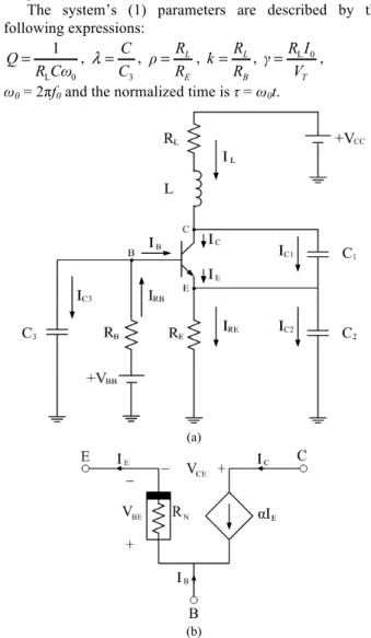
2. The Proposed Colpitts Circuit
The proposed circuit, which is used, is a fourth order Colpitts-type circuit, as it is shown in Fig.1(a). In more details, this circuit is based on the standard Colpitts circuit [21], which its base is biased by the second voltage source VBB through the resistor RB and this branch is in parallel with
the capacitor C3.
In order to derive a mathematical model that is tractable both analytically and numerically, two basic assumptions, are considered:
• Firstly, all capacitors, inductor, and resistors are assumed to be linear.
• Secondly, the transistor Q is modeled by a nonlinear resistor RN and a linear current-controlled current source αIE, as shown in Fig.1(b).
Denoting by (x, y, z) the voltages VCi (i = 1, 2, 3) across
the capacitors Ci (i = 1, 2, 3) and by (w) the voltage across
the resistor RL, the Kirchhoff’s electric circuit laws can be
applied to the schematic diagram of Fig.1(a) to obtain the following fourth-order autonomous dynamical system.
[
]
(
)
(
)
[
]
1 1 1 2 BB CC dxQ w F dτ
dy
Q w F y
dτ dz
λQ kV F kz
dτ dw
V x y w
dτ Q α α ρ α ⎧ = − ⎪ ⎪ ⎪ = ⎡ + − − ⎤ ⎣ ⎦ ⎪⎪ ⎨ ⎪ = ⎡⎣ − − − ⎤⎦ ⎪ ⎪ ⎪ = − − − ⎪⎩ (1)
As it is mentioned, the BJT is modeled by a voltage-controlled nonlinear resistor RN and a linear
current-controlled current source, while the parasitic and the reverse effects are discarded [22]. This BJT model is illustrated in Fig.1(b), where α denotes the Common-Base (CB) short-circuit forward current gain of the BJT. The nonlinear characteristic of RN is approximated by an exponential
function:
( ) e 1
BE T
V V Ε f VBE IS
Ι = = ⎛⎜⎜ − ⎞⎟⎟
⎝ ⎠
(2)
which is modeled, in this paper, by using the following piece-wise linear function:
, if
( )
0, if
BE Th
0 BE Th
BE T
BE Th
V V
I V V
f V V
V V Ε Ι ⎧ ⎛ − ⎞ ≥ ⎪ ⎜ ⎟ = =⎨ ⎝ ⎠ ⎪ < ⎩ (3)
with V = z – y and V V ⎡ln⎛aI0⎞ 1⎤
= ⎢ ⎜ ⎟− ⎥. Also, I is the
VT = kbT/q is the thermal voltage, with kb the Boltzmann
constant, T the absolute temperature expressed in Kelvin, and q the electron charge. Note that VT ≈ 27 mV at room
temperature (300oK).
The system’s (1) parameters are described by the following expressions:
L 0
1 Q
R Cω
= ,
3
C C
λ= , L
E
R
ρ
R
= , L B
R k
R
= , L 0
T
R I
γ
V
= ,
ω0 = 2πf0 and the normalized time is τ = ω0t.
(a)
(b)
Fig. 1. (a) The schematic of the proposed Colpitts-type circuit and
(b) the transistor model in CB configuration.
The numerical simulation of system’s equation (1) was done using a fourth-order Runge-Kutta algorithm. For the simulation the following values of circuit’s parameters have been used: VCC = 12 V, VBB = 7 V, I0 = 15 mA,
IS =
15
14.34 10⋅ − A (for Q2N2222), RL = 20 Ω, RB = 400 Ω,
RE = 1000 Ω, C = C1 = C2 = 56.5 nF, C3 = 107.8 nF, α = 0.99379 (the forward current gain of the device is β = 160), while L played the role of the control parameter.
To understand the behavior of such a dynamical system with the variation of a parameter, the bifurcation diagram can be used. There are many ways to extract this diagram (using the Poincaré surface plot, plot the maxima of the time-series, etc). However, in this work the bifurcation diagram is obtained by plotting the points of intersection of
the trajectory with a selected section plane (w = 0 with dw/dt > 0).
144
doubling again for 129 µΗ < L < 289.5 µΗ and finally, after a reverse period doubling the system undergoes to a period-1 steady state for L > 445 µΗ. These forward and reverse period-doubling sequences, as parameter L increases in a monotone way, is called antimonotonicity [23-28].
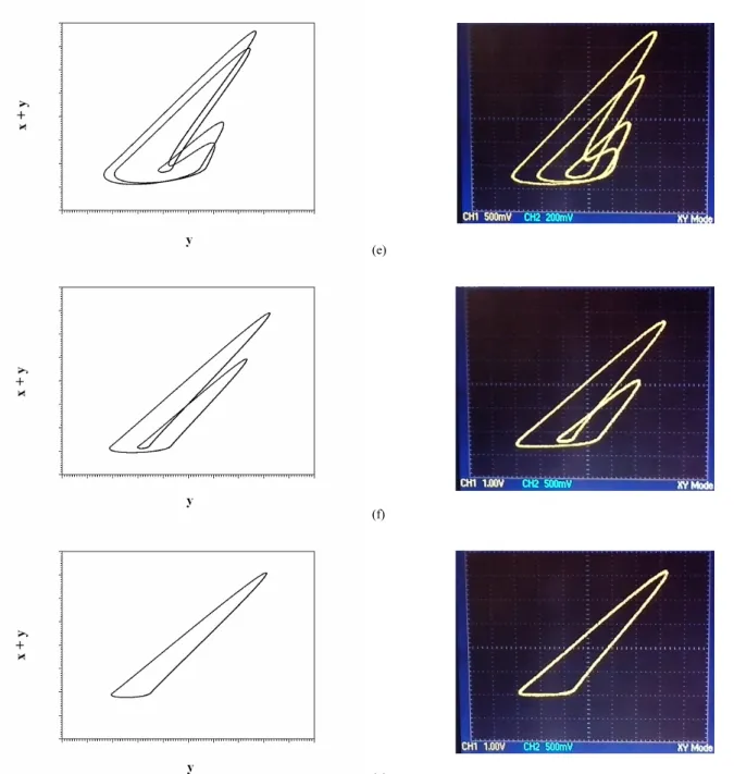
In Fig.3 the phase portraits of the collector voltage (x + y) versus the emitter voltage y, produced by circuit’s
simulation process as well the respective experimental by using the digital oscilloscope TDS 2024B of Tektronix, are shown for various values of the inductor L. Furthermore, the initial conditions of a system (1) in the simulation are: (x0, y0, z0, w0) = (0.5, 0.2, -0.5, 0.0). The very good agreement between the simulation and experimental results can be observed.
Fig. 2. The bifurcation diagram of y vs. L. The chaotic region is shown
more clearly in the inset figure.
3. The Coupling Schemes
Since nonlinear circuits and especially chaotic circuits exhibit high sensitivity on initial conditions and thus, if they are identical and, possibly, starting from almost the same initial points, following trajectories which rapidly become uncorrelated, appropriate techniques should be set up to obtain synchronization. Such techniques to couple two or more chaotic systems can be mainly divided into two classes: bidirectional or mutual coupling and drive-response or unidirectional coupling [29]. In the first case, both circuits are connected and each circuit influences the dynamics of the other one, while on the contrary in unidirectional coupling one system drives another one called the response or slave system. So, the mutually coupled systems show always more complex dynamic behavior.
In this section the coupling schemes (bidirectional and unidirectional) between two identical Colpitts circuits of system (1) are studied. As coupling nodes, the collectors of each circuit have been chosen. The reason for the choice of these nodes, instead of i.e. the emitters, is the totally different, from the literature, dynamical system which is produced.
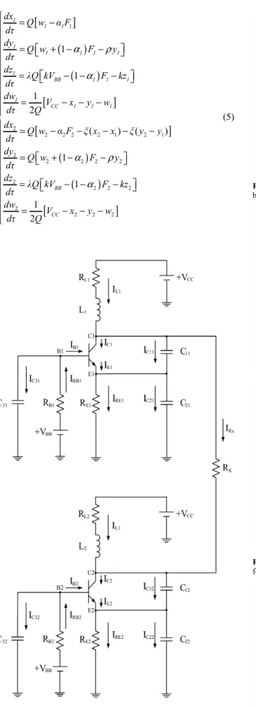
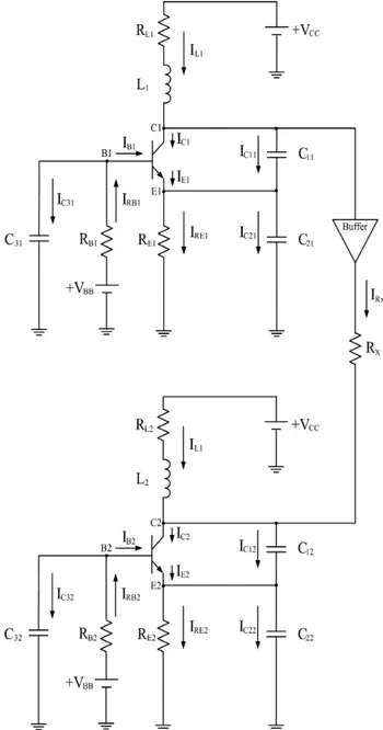
3.1. The Mutual Coupling Scheme
The schematic diagram of this coupling scheme is given in Fig. 4. This coupling is achieved via a linear resistor RX
connected between the collector nodes of each circuit. By applying Kirchooff’s laws, the following system of differential equations is obtained.
[
]
(
)
(
)
[
]
[
]
(
)
(
)
1 22 2 2 2 1 2 1
2
2 2 2 2
2
2 2 2
2 ( ) ( ) 1 1 1 2 ( ) ( ) 1 1 1 2 1
1 1 1 2 1 2
1
1 1 1 1
1
BB 1 1 1
1
CC 1 1 1
BB
CC dx
Q w αF ξ x x ξ y y
dτ
dy
Q w F y
dτ
dz
λQ kV F kz dτ
dw
V x y w
dτ Q
dx
Q w αF ξ x x ξ y y
dτ
dy
Q w F y
dτ
dz
λQ kV F kz dτ
dw
V
dτ Q
α ρ α α ρ α = − − − − − = ⎡⎣ + − − ⎤⎦ = ⎡⎣ − − − ⎤⎦ = − − − = − − − − − = ⎡⎣ + − − ⎤⎦ = ⎡⎣ − − − ⎤⎦
=
[
−x2 y2 w2]
⎧ ⎪ ⎪ ⎪ ⎪ ⎪ ⎪ ⎪ ⎪ ⎪ ⎪ ⎨ ⎪ ⎪ ⎪ ⎪ ⎪ ⎪ ⎪ ⎪ ⎪ − − ⎪ ⎩ (4)
The first four equations of system (4) describe the first of the two coupled identical Colpitts circuits, while the other four describe the second one. The bipolar transistors are chosen to have the same forward current gain (β1 = β2 = 160). So, α1 = α2. Also, the parameter ξ = RL/RX is the
coupling coefficient and it is present in the equations of both circuits, since the coupling between them is mutual. As it is shown in this system, there are two terms, in the first and fifth equation, depending on the coupling coefficient ξ, instead of one which is obtained usually in the bidirectionally coupling scheme.
In Fig. 5 the bifurcation diagram of the signal’s difference (y2 – y1) versus the coupling coefficient ξ is
shown. This diagram is produced by increasing the coupling coefficient ξ, from ξ = 0 (uncoupled system) to ξ = 2 with
step Δξ = 0.002. The initial conditions of the system are (x10, y10, z10, w10, x20, y20, z20, w20) = (0.5, 0.2, –0.5, 0.0, 0.3,
0.0, –0.3, 0.2), while the circuits’ parameters are the same as in the previous section. Also, the value of the inductor L is chosen equal to 58.5 µH in order for each circuit to be in a chaotic mode.
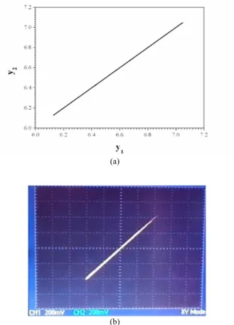
From the bifurcation diagram’s analysis, very interesting synchronization phenomena, concerning the coupled circuits, are obtained. In more details, the system begins from a chaotic desynchronization state for ξ = 0 and very rapidly is driven to a region where the system is in periodic state (i.e. for ξ = 0.028). Specifically, in this region the system shows a period-2 steady state, as it can be observed from the phase portrait of y2 versus y1 in Fig. 6(a).
Also, this behavior drives us to the conclusion that the system shows the phenomenon of anti-phase synchronization [30-31]. This synchronization phenomenon is observed when a coupled system is in a phase locked (periodic) state (Fig. 6(b)), depending on the coupling coefficient and it can be characterized by a π-phase delay.
So, the periodic signals of each coupled circuit have a
time lag τ = 0.0155 ms, which is equal to T/2, where T = 0.0310 ms is the period of the signals (Fig.7(a)).
(a)
(b)
(c)
146 (e)
(f)
(g)
Fig. 3. Phase portraits of (x + y) vs. x from the simulation and experiment respectively. (a) L = 25 µH, (b) L = 40 µH, (c) L = 50 µH, (d) L = 58.5 µH,
(e) L = 200 µH, (f) L = 400 µH, (g) L = 500 µH.
[
]
(
)
(
)
21/ 2
2 2
2
( ) ( )
( )
( ) ( )
2 1
1
y t y t
S
y t y t
τ
τ = + −
⎡ ⋅ ⎤
⎣ ⎦
(5)
The same phenomenon of anti-phase synchronization is
also observed in the second periodic region of ξ∈[0.09, 0.36], as it is confirmed from Figs. 8. By using
again the similarity function of Eq.(5) the same time lag, as in the previous case, has been calculated.
Next, the system is driven to a quasi-periodic behavior (Fig. 9), as it is found by calculating the system’s Lyapunov exponents for ξ = 0.7 (LE1 = 0, LE2 = 0, LE3 = –0.04241,
LE4 = –0.04695, LE5 = –0.05199, LE6 = –0.46153,
LE7 = –1.28539, LE8 = –1.89186). The two zero Lyapunov
exponents is a sign of a quasi-periodic behavior.
As the coupling factor increases the system gradually exits from the quasi-periodic region and for ξ∈[1.42, 1.76]
the coupled system enters in a region of periodic behavior, as it is observed from Figs. 10, in which the simulation and the respective experimental phase portrait of y2 versus y1, for ξ = 1.5 are shown. This region is divided in two sub-regions in which the system is driven by sudden jumps.
Finally, for ξ > 1.76 the two coupled circuits are in a chaotic synchronization state (Fig. 11), in which the difference signal y2 – y1 tends to zero.
3.2. The Unidirectional Coupling Scheme
[
]
(
)
(
)
[
]
[
]
(
)
(
)
[
]
1
2
2 2 2 2 1 2 1
2
2 2 2 2
2
2 2 2
2
2 2 2
1
1
1 2
( ) ( )
1
1
1 2
1
1 1
1
1 1 1 1
1
BB 1 1 1
1
CC 1 1 1
BB
CC dx
Q w αF
dτ dy
Q w F y
dτ dz
λQ kV F kz
dτ dw
V x y w
dτ Q
dx
Q w αF ξ x x ξ y y
dτ dy
Q w F y
dτ dz
λQ kV F kz
dτ dw
V x y w
dτ Q
α ρ
α
α ρ
α ⎧
= −
⎪ ⎪
⎪ = ⎡ + − − ⎤
⎣ ⎦
⎪ ⎪
⎪ = ⎡ − − − ⎤
⎣ ⎦
⎪ ⎪
= − − −
⎨
= − − − − −
= ⎡⎣ + − − ⎤⎦
= ⎡⎣ − − − ⎤⎦
= − − −
⎪ ⎪ ⎪ ⎪ ⎪ ⎪ ⎪ ⎪ ⎪ ⎪ ⎪ ⎪ ⎩
(5)
Fig. 4. The schematic of the bidirectionally coupled Colpitts-type
Fig. 5. The bifurcation diagram of y2 – y1 vs. ξ, in the case of
bidirectional coupling.
(a)
(b)
Fig. 6. Simulation phase portraits of (a) y2 vs. y1 and (b) x1,2 + y1,2 vs. y1,2
148 (a)
(b)
Fig. 8. (a)Simulation phase portraits of y2 vs. y1 and (b) time-series of
y1 and y2, for (a) ξ = 0.258 (anti-phase synchronization).
Fig. 9. (a)Simulation phase portraits of y2 vs. y1 for ξ = 0.7
(quasi-periodic behavior).
(a) (continued)
(b)
Fig. 10. (a) Simulation and (b)experimental phase portraits of y2 vs. y1,
forξ = 1.5.
(a)
(b)
Fig. 11. (a), (b) Simulation and experimental phase portraits of
(a) y2 vs. y1, for ξ = 2 (chaotic synchronization).
By using again the bifurcation diagram of y2 – y1 versus
the coupling coefficient ξ, for the same set of circuits’ parameters and initial conditions, as in the previous coupling scheme, an interest dynamical behavior is observed.
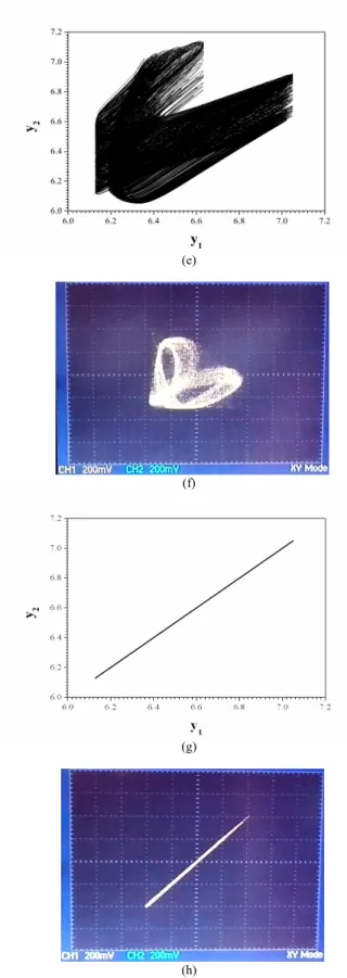
The system begins from the chaotic desynchronization state (Fig. 14(a) & (b)), but unexpectedly the system’s chaotic region is interrupted by a small window of chaotic synchronization behavior (Fig. 14(c) & (d)).
However, this state is unstable and the system enters again in an extended chaotic desynchronization region (Fig. 14(e) & (f)), which is gradually reduced and finally after a sudden jump for ξC = 4.0, the system is driven to a permanent chaotic synchronization state (Fig. 14(g) & (h)).
Fig. 12. The schematic of the unidirectionally coupled Colpitts-type
circuits, via a linear resistor RX and a buffer.
Fig. 13. The bifurcation diagram of y2 – y1 vs. ξ, in the case of
unidirectional coupling.
(a)
(b)
(c)
150 (e)
(f)
(g)
(h)
Fig. 14. Simulation and experimental phase portraits of y2 vs. y1 for
(a) ξ = 0.06, (b) ξ = 0.16, (c) ξ = 0.8 and (d) ξ = 4.2.
4. Conclusion
In this paper, the case of resistively coupling between two identical nonlinear chaotic nonlinear circuits has been studied. As coupling schemes the bidirectional and unidirectional cases were chosen. Also, the choice of the coupling nodes was done based on the fact that these coupled systems produce dynamical systems, with different structure, in regard to other similar works.
As a circuit, a modification of the most well-known nonlinear circuit that can operate in a wide range of radiofrequencies, the Colpitts oscillator, is chosen. In this work, circuit’s base is biased by a second voltage source which is parallel with a third capacitor.
The simulation and the experimental results, in both coupling cases, show a variety of dynamical phenomena, depending on the value of the coupling coefficient.
In the case of bidirectional coupling scheme the system presented a complicated dynamical behavior because each circuit influences the dynamics of the other one. So, the classical route from chaotic desynchronization to chaotic synchronization was interrupted by regions in which the coupled system was in a chaotic, periodic or quasi-periodic state. Also, in the periodic regions, for low values of the coupling coefficient, the anti-phase synchronization phenomenon, between the coupled identical Colpitts-type circuits, was observed.
On the other hand, in the case of unidirectional coupling scheme, a more simple and slow route from chaotic desynchronization to chaotic synchronization, was observed. This occurs because only the first circuit affects the dynamics of the second circuit. However, the extended chaotic desynchronization region was interrupted by an unexpected window of unstable chaotic synchronization state, for extremely low values of the coupling coefficient, which has been reported for the first time. This phenomenon occurred because of coupling system’s structure.
______________________________
References
1. A. Garliauskas, Neural network chaos analysis. Nonlinear Analysis: Modelling and Control, Vilnius, IMI, vol. 3, pp. 1-14 (1998).
2. Ch.K. Volos, I.M. Kyprianidis, I.N. Stouboulos, Image encryption process based on chaotic synchronization
phenomena, Signal Processing, vol. 93(5), pp. 1328-1340 (2013).
4. B. Van der Pol and J. Van der Mark, Frequency demultiplication, Nature, vol. 120, pp. 363-364 (1927). 5. Y. Ueda and N. Akamatsu, Chaotically transitional phenomena
in the forced negative-resistance oscillator, IEEE Transactions on Circuits & Systems, vol. 28, pp. 217-224 (1981).
6. S.D. Brorson, D. Dewey, and P.S. Linsay, Self-replicating attractor of a driven semiconductor oscillator, Physical Review A, vol. 28, pp. 1201-1203 (1983).
7. G.-Q. Zhong, F. Ayrom, Experimental confirmation of chaos from Chua's circuit, International Journal of Circuit Theory & Applications, 13(1), 93 (1985).
8. E.H. Colpitts, Oscillation generator, United Stated Patent, 1918. 9. K.M. Cuomo, S.H. Isabelle, Spread spectrum modulation and
signal masking using synchronized chaotic systems, MIT Technical Report, 1992.
10. N. Rulkov, M. Sushchik, L. Tsimring, and A. Volkovsky, Digital communication using chaotic-pulse-position modulation, IEEE Transactions on Circuits & Systems I: Fundamental Theory and Applications, vol. 48, pp. 1436-1444 (2001).
11. F. Dachselt and W. Schwarz, Chaos and cryptography, IEEE Transactions on Circuits & Systems I: Fundamental Theory and Applications, vol. 48, pp. 1498-1509 (2001).
12. G. Heidari-Bateni and C.D. McGillem, A chaotic direct-sequence spread spectrum communication system, IEEE Transactions on Communications, vol. 42, pp. 1524-1527 (1994).
13. M. Wada, J. Kawata, Y. Nishio, and A. Ushida, Ber estimation of a chaos communication system including modulation demodulation circuits, IEICE Transanction on Fundamentals, vol. E83-A, pp. 563-566 (2000).
14. L.M. Pecora and T.L. Carroll, Synchronization in chaotic systems, Physics Review Letters, vol. 64, pp. 821-824 (1990). 15. I.M. Kyprianidis, Ch.K. Volos, I.N. Stouboulos, and J.
Hadjidemetriou, Dynamics of two resistively coupled Duffing – type electrical oscillators, Int. J. Bifurc. Chaos, vol. 16, pp. 1765-1775 (2006).
16. I.M. Kyprianidis, Ch.K. Volos, S.G. Stavrinides, I.N. Stouboulos, and A.N. Anagnostopoulos, On – off intermittent synchronization between two bidirectional coupled double Scroll circuits, Commun. Nonlinear Sc. Numer. Simulat., vol. 15, pp. 2192-2200 (2010).
17. I.M. Kyprianidis, Ch.K. Volos, S.G. Stavrinides, I.N. Stouboulos, and A.N. Anagnostopoulos, Master – slave double – scroll circuit incomplete synchronization, J. Engineering Science & Technology Review, vol. 3, pp. 41-45 (2010).
18. Ch.K. Volos, I.M. Kyprianidis, and I.N. Stouboulos, Various synchronization phenomena in bidirectionally coupled double scroll circuits, Commun. Nonlinear Sc. Numer. Simulat., vol. 16. pp. 3356-3366 (2011).
19. Ch.K. Volos, I.M. Kyprianidis, and I.N. Stouboulos, Anti-phase and inverse π-lag synchronization in coupled Duffing-type circuits, International Journal of Bifurcation and Chaos, vol. 21(8), pp. 2357-2368 (2011).
20. Ch.K. Volos, I.M. Kyprianidis, and I.N. Stouboulos, An universal phenomenon in mutually coupled Chua’s circuit family, Journal of Circuits, Systems and Computers, vol. 23(2), pp. 1450028/1-20 (2014).
21. M.P. Kennedy, Chaos in the Colpitts oscillator, IEEE Transactions on Circuits & Systems, vol. CAD-41, pp. 771-774 (1994).
22. S. Sedra and K. Smith, Microelectronic circuits, Oxford University Press, New York (1998).
23. M. Bier and T.C. Bountis, Remerging Feigenbaum trees in dynamical systems, Phys. Lett. A, vol.104, pp. 239-244 (1984). 24. I.M. Kyprianidis, P. Haralabidis, I.N. Stouboulos, and T.
Bountis, Antimonotonicity and chaotic dynamics in a fourth oder autonomous nonlinear electric circuit, Int. J. Bifurcation & Chaos, vol.10, pp. 1903-1915 (2000).
25. I.M. Kyprianidis and M.E. Fotiadou, Complex dynamics in Chua’s canonical circuit with a cubic nonlinearity, WSEAS Trans. Circuits Syst., vol.5, pp. 1036-1043. (2006).
26. I.M. Kyprianidis, Antimonotonicity in Chua’s canonical circuit, In. Proc. of the 5th WSEAS Int. Conf. on Non-Linear Analysis, Non-Linear Systems and Chaos, Bucarest, Romania, pp. 75-80 (2006).
27. I.M. Kyprianidis, New chaotic dynamics in Chua’s canonical circuit, WSEAS Trans. Circuits Syst., vol.5, pp. 1626-1633 (2006).
28. I.M. Kyprianidis, A.T. Makri, I.N. Stouboulos, and Ch.K. Volos, Antimonotonicity in a FitzHugh-Nagumo type circuit, In Recent Advances in Finite Differences and Applied & Computational Mathematics, Proc. 2nd International Conference on Applied and Computational Mathematics (ICACM '13), pp. 151-156 (2013).
29. L. Fortuna, M. Frasca, and M.G. Xibilia, Chua’s circuit implementations: Yesterday, Today and Tomorrow, World Scientific, Singapore, (2009).
30. L.Y. Cao and Y.C. Lai, Antiphase synchronism in chaotic systems, Physical Review E, vol. 58(1), pp. 382-386 (1998). 31. Ch.K. Volos, I.M. Kyprianidis, and I.N. Stouboulos, A gallery of
synchronization phenomena in resistively coupled non-autonomous chaotic circuits, Journal of Engineering Science and Technology Review, vol. 6(4), pp. 15-23 (2013).