www.the-cryosphere.net/3/85/2009/
© Author(s) 2009. This work is distributed under the Creative Commons Attribution 3.0 License.
The Cryosphere
Transient thermal effects in Alpine permafrost
J. Noetzli and S. Gruber
Glaciology, Geomorphodynamics and Geochronology, Department of Geography, University of Zurich, Switzerland Received: 26 February 2008 – Published in The Cryosphere Discuss.: 2 April 2008
Revised: 9 March 2009 – Accepted: 27 March 2009 – Published: 27 April 2009
Abstract. In high mountain areas, permafrost is important because it influences the occurrence of natural hazards, be-cause it has to be considered in construction practices, and because it is sensitive to climate change. The assessment of its distribution and evolution is challenging because of highly variable conditions at and below the surface, steep topog-raphy and varying climatic conditions. This paper presents a systematic investigation of effects of topography and cli-mate variability that are important for subsurface temper-atures in Alpine bedrock permafrost. We studied the ef-fects of both, past and projected future ground surface tem-perature variations on the basis of numerical experimenta-tion with simplified mountain topography in order to demon-strate the principal effects. The modeling approach applied combines a distributed surface energy balance model and a three-dimensional subsurface heat conduction scheme. Re-sults show that the past climate variations that essentially in-fluence present-day permafrost temperatures at depth of the idealized mountains are the last glacial period and the ma-jor fluctuations in the past millennium. Transient effects from projected future warming, however, are likely larger than those from past climate conditions because larger tem-perature changes at the surface occur in shorter time peri-ods. We further demonstrate the accelerating influence of multi-lateral warming in steep and complex topography for a temperature signal entering the subsurface as compared to the situation in flat areas. The effects of varying and un-certain material properties (i.e., thermal properties, porosity, and freezing characteristics) on the subsurface temperature field were examined in sensitivity studies. A considerable influence of latent heat due to water in low-porosity bedrock was only shown for simulations over time periods of decades to centuries. At the end, the model was applied to the
to-Correspondence to: J. Noetzli ([email protected])
pographic setting of the Matterhorn (Switzerland). Results from idealized geometries are compared to this first example of real topography, and possibilities as well as limitations of the model application are discussed.
1 Introduction
In Alpine environments, permafrost is a widespread thermal subsurface phenomenon. Permafrost is defined as material of the lithosphere that remains at or below 0◦C for at least
The understanding of three-dimensional and transient sub-surface temperature fields below steep topography can be improved by numerical modeling that accounts for two- and three-dimensional effects (e.g., Safanda, 1999; Kohl et al., 2001; Wegmann et al., 1998).
Noetzli et al. (2007b) have shown that in complex topog-raphy ground surface temperatures (GST) alone do not suffi-ciently indicate the thermal conditions at depth (when speak-ing of “at depth” in this paper, we refer to depths deeper than the zero annual amplitude – ZAA): Because of existing lat-eral heat fluxes, permafrost can occur at locations with pos-itive GST even if conditions are stationary. Stationary con-ditions, however, do not describe the situation found in na-ture since transient effects of past climate periods addition-ally modify the subsurface temperature field. In the Swiss Alps, permafrost thickness ranges from a few meters up to several hundreds of meters below the highest peaks (such as the Monte Rosa massif; L¨uthi and Funk, 2001), and time scales involved in deep permafrost changes can be in the range of millennia even without the retarding effect of latent heat (e.g., Lunardini, 1996; Kukkonen and Safanda, 2001; Mottaghy and Rath, 2006). Consequently, the influence of past cold periods such as the last Ice Age are likely to persist in permafrost temperatures in the interior of high mountains (Haeberli et al., 1984, Kohl, 1999; Kohl and Gruber, 2003). The more recent but smaller 20th century warming (Haeberli and Beniston, 1998; Beniston, 2005) currently affects ground temperatures in the upper decameters. That is, a realistic simulation of today’s thermal state of mountain permafrost cannot be based on current GST alone, but it is necessary to initialize the model far enough in the past. A corresponding initialization procedure has to include the past climate varia-tions that influence current subsurface temperatures. Further, the modeling of transient temperature fields is essential to as-sess possible permafrost temperatures in the coming decades and centuries.
The combined effects of steep topography and transient paleoclimatic signals on the subsurface temperature fields in the interior of Alpine peaks have not been systematically studied so far. In this paper, we first analyze how big the in-fluence of past climate conditions is on the present-day ther-mal state of mountain permafrost. And secondly, we con-sider a simplified scenario of future climate change in order to estimate their effect. Our study is based on numerical ex-perimentation with simplified topography and typical values of surface and subsurface conditions because the situation in nature is highly variable and complex. The results of such idealized simulations can be used to identify the principal effects and will contribute to our understanding of the three-dimensional distribution of mountain permafrost, its thermal state today, and its possible evolution in the future. They should be seen as a step towards assessing natural and more complicated situations. Results will also be useful to decide on the initialization procedure required for the modeling of permafrost temperatures in high-mountains. At the end, the
model is applied to the topographic setting of the Matterhorn (Switzerland). Results from idealized geometries are com-pared to this first example of real topography, and possibili-ties as well as important limitations of the model applications are discussed.
2 Background and approach 2.1 Background
Many studies point to significant temperature depressions in the deeper subsurface, which are caused by past cold climate conditions (e.g., Haeberli et al., 1984; Safanda and Rajver, 2001). That is, actual subsurface temperatures are colder than for a stationary temperature field that corresponds to current climate conditions. The depth to which a ground sur-face temperature variation is perceivable is determined by its amplitude and duration, as well as by the thermal proper-ties of the subsurface. In modeling studies, such temperature anomalies are usually computed as deviations of actual ther-mal conditions from equilibrium conditions (e.g., Pollak and Huang, 2000; Beltrami et al., 2005). In a first approach, they can be calculated by superposition of stepwise temperature changes using analytical heat transfer solutions (e.g., Birch, 1948; Carslaw and Jaeger, 1959). Based on this technique, an assumed 10◦C cooler surface temperature during the last
Pleistocene Ice Age (ca. 70–100 ky BP) still causes a tem-perature depression of more than 4◦C at a depth of 1000 m
(Kohl, 1999). Haeberli et al. (1984) have estimated a ground temperature depression from the last cold period of 5◦C at a
2.2 Approach
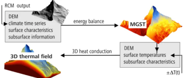
The modeling of subsurface temperatures in high-mountains is complex because temperature fields are significantly in-fluenced by (i) spatially variable GST, (ii) spatially vari-able properties of the subsurface, (iii) three-dimensional ef-fects caused by steep terrain geometry, and (iv) the evolu-tion of GST in the past. In this study, we used and further developed the modeling procedure described by Noetzli et al. (2007a, b), which has been designed and validated (Noet-zli 2008, Noet(Noet-zli et al., 2008) for use in steep mountain to-pography: A distributed surface energy balance model to cal-culate ground surface temperatures and a three-dimensional heat-conduction model are combined for forward simulation of a subsurface temperature field (Fig. 1).
Heat transfer is mainly conductive in bedrock permafrost and is driven by the spatial and temporal temperature vari-ations at the surface and the heat flow from the interior of the earth. The distributed surface energy balance model used enables a sound calculation of spatially variable surface tem-peratures in steep terrain (Gruber et al., 2004b). Further pro-cesses such as advection by fluid flow can, as a first approx-imation, be neglected (e.g., Kukkonen and Safanda, 2001). Accordingly, we considered a purely conductive transient thermal field with the modeled surface temperatures as up-per, and the geothermal heat flux as lower boundary condi-tion. More details on the models, their validation, and their settings are given in Sect. 3.
To account for the evolution of GST in the past, we ini-tialize the subsurface temperature field based on a prescribed GST history using a steady state solution for the GST con-ditions at the start time. We applied different GST histories, which we compiled based on published changes in air tem-peratures and the simplifying assumption that GST follow these changes closely. That is, effects from changes in other components of the surface energy balance, snow cover, or surface characteristics are not considered. Temporal vari-ations of surface temperatures penetrate downward with a considerable time lag and with amplitudes diminishing ex-ponentially with depth. In this study, we ignore seasonal temperature variations, which may penetrate down to about 10–15 m in solid and dry bedrock (Gruber et al., 2004a), and only consider long-term variations with time scales of decades to millennia, which influence temperatures at greater depth. Such long-term variations still occur on much shorter time scales than the geological processes that determine the geothermal heat flow. The past climatologic variations are therefore treated as transient effects of the upper boundaries in our model, and the lower basal heat flow boundary con-dition is kept constant (cf. Pollak and Huang, 2000). The lack of information concerning the most important subsur-face characteristics that influence conductive heat transport (thermal properties, porosity, freezing characteristics, etc.) is approached by using model assumptions based on sensitivity studies.
Fig. 1. Mean ground surface temperatures (MGST) are calculated
based on a surface energy balance model (TEBAL). They are used as upper boundary condition in a three-dimensional finite element heat conduction scheme (within COMSOL) to compute the subsur-face temperature field. For transient simulations the evolution of the surface temperatures is prescribed.
We performed the basic simulations for a simplified ridge, the most common feature comprising Alpine topography (cf. Noetzli et al., 2007). A ridge of 1000 m height was set to an elevation of 3500 m a.s.l. and east-west orientation. Hence, it has a warm south-facing and a cold north-facing slope, which induces a subsurface temperature field with steeply inclining isotherms in the uppermost part (cf. Fig. 3). A threshold for the slope of steep bedrock is often set at about 37◦ (e.g., Gruber and Haeberli, 2007). Couloirs with this
steepness, however, can often contain a significant amount of snow or debris, and because we do not consider any surface cover in the idealized settings, we set the slope value to 50◦.
In order to study the influence of terrain geometry, we varied the topographic factors (i.e., elevation and slope angle) of the two-dimensional ridge. Finally, we compared the results for a ridge topography to those for a flat and one-dimensional plain and a three-dimensional mountain peak represented by a pyramid. The use of a distributed energy balance approach is not essential for the experimentation presented here, and a reasonable parameterization for GST would suffice. For model application to more complex topography, however, the spatial distribution of GST cannot be easily parameterized and its sound calculation is crucial, because it drives the di-rection and magnitude of subsurface heat fluxes (Gruber et al., 2004c; Noetzli et al., 2007). For consistency and in or-der to demonstrate the entire modeling procedure, GST are calculated based on the distributed energy balance model for simulations with both, idealized and real topography.
3 Temperature modeling
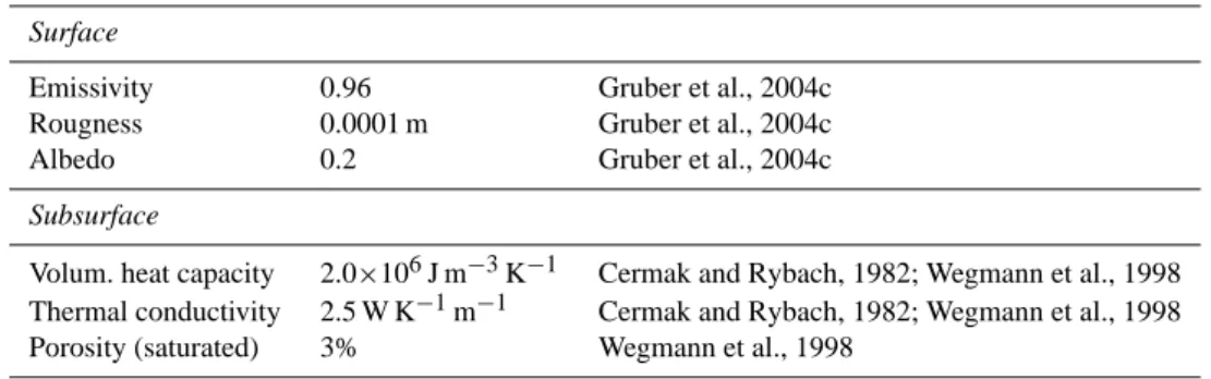
Table 1. Surface and subsurface properties assumed in the experimentation runs.
Surface
Emissivity 0.96 Gruber et al., 2004c Rougness 0.0001 m Gruber et al., 2004c Albedo 0.2 Gruber et al., 2004c
Subsurface
Volum. heat capacity 2.0×10⁶J m−3K−1 Cermak and Rybach, 1982; Wegmann et al., 1998
Thermal conductivity 2.5 W K−1m−1 Cermak and Rybach, 1982; Wegmann et al., 1998 Porosity (saturated) 3% Wegmann et al., 1998
(Gruber, 2005; Stocker-Mittaz, 2002) and validated (Gru-ber, 2005; Gruber et al., 2004b; Noetzli et al., 2007b) for the calculation of near-surface temperatures in steep rock slopes in the Alps and was successfully applied in previous studies on bedrock permafrost (e.g., Gruber et al., 2004a, b; Noet-zli et al., 2007b; Salzmann et al., 2007). Mean ground sur-face temperatures (MGST) are computed using gridded dig-ital elevation models (DEMs) of the topography considered and with hourly climate time series from a high elevation meteo station. In this paper, we used the data from Cor-vatsch at 3315 m a.s.l. in the Upper Engadine (Data source: MeteoSwiss) for the period 1990–1999 AD. We further ref-erence this period as “today” or “present”. Surface and sub-surface properties for bedrock were set to typical values of Alpine rock according to Noetzli et al. (2007a; Table 1). The influence of their possible variation was additionally assessed in sensitivity studies (cf. Sects. 4.1.2 and 4.2.2.) For simpli-fication purposes and because most steep rock slopes do not accumulate a thick snow cover during winter, we neglect the simulation of the snow cover for the numerical experiments. 3.2 Heat conduction and subsurface temperatures
As described above (Sect. 2.2), we considered a conduc-tive three-dimensional transient thermal field (Carslaw and Jaeger, 1959) in an isotropic and homogeneous medium un-der complex topography. The thermal properties of the sub-surface were set based on published values (Cerm´ak and Ry-bach, 1982; Wegmann et al., 1998; Safanda, 1999) (cf. Ta-ble 1).
Ice contained in the pore space and crevices delays the re-sponse to surface warming by the consumption of latent heat, which may influence the time and depth scales of permafrost degradation by orders of magnitude even in low porosity rock (Wegmann et al., 1998; Romanovsky and Osterkamp, 2000; Kukkonen and Safanda, 2001). This effect can be handled in heat transfer models by introducing an apparent heat ca-pacity. We used the approach described by Mottaghy and Rath (2006): The apparent heat capacity substitutes the heat capacity in the heat transfer equation within the freezing in-tervalw. The freezing intervalwdescribes the temperature
range, where phase transition takes place and unfrozen wa-ter is present, and which relates to the steepness of the un-frozen water content curve. The parameterwmakes it
pos-sible to account for a variety of ground conditions (Mot-taghy and Rath, 2006): Values ofw typically range from
0.5 K for material such as sand to 2 K for material such as bentonite (Anderson and Tice, 1972; Williams and Smith, 1989), but information on bedrock material is sparse. Weg-mann (1998) found that most of the interstitial ice in the rock of the Jungfrau East Ridge, Switzerland, freezes at –0.3◦C,
which indicates a small freezing interval with a steep curve and a low value ofw. A further important factor is the
poros-ity of the material, for which we assumed 3% (volume frac-tion, saturated conditions) to be a reasonable value to inves-tigate the principal effects (cf. Wegmann et al., 1998).
The commercial finite-element (FE) modeling package COMSOL Multiphysics was used for forward modeling of subsurface rock temperatures (Noetzli et al., 2007a). The heat conduction module included in this software has been successfully used for the simulation of borehole temperature profiles in the Schilthorn ridge, Switzerland (Noetzli et al., 2008) and the Zugspitze, Germany (Noetzli, 2008). The FE mesh for the topographies was created with increasing verti-cal refinement from 250 m at depth to 10 m for elements clos-est to the surface. In order to avoid effects from the model boundaries, a rectangle box of 2000 m height and thermal in-sulation at its sides was added below the geometry. The FE mesh consisted of ca. 1500 elements for a ridge, and of about 25 000 elements for a pyramid. The lower boundary condi-tion was set to a uniform heat flux of 80 mW m−2 (Medici and Rybach, 1995), and for the upper boundary conditions the modeled MGSTs were given. The model was run with time-steps of 1 year for simulations over a period of more than 1000 years, and with time steps of 10 days for shorter periods. Sensitivity runs with higher refinement of the FE mesh, a lower boundary condition set at greater depth, and smaller time steps did not considerably change any of the re-sults (i.e., the maximum absolute difference in modeled tem-peratures was below 0.1◦C).
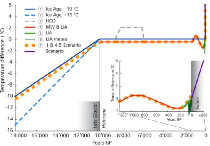
Fig. 2. For the initialization runs, surface temperature histories of
diverse lengths and temporal resolutions were used. Based on the results obtained, an initialization curve for further simulations was compiled (thick dashed orange line). Scenarios were calculated as-suming a uniform linear warming of+3◦C/100 y. MW=Medieval
Warmth, HCO=Holocene Climate Optimum, LIA=Little Ice Age.
conduction simulated in COMSOL. Because measurements of entire three-dimensional temperature fields in mountains are hardly feasible, three different validation steps have been taken in order to gain confidence in the modeling results (Noetzli, 2008). They include: (1) comparison with field data measured at or near the surface, (2) comparison with tem-perature profiles from boreholes, and (3) sensitivity studies. For (1) and (2) we refer to the detailed descriptions and re-sults presented in Gruber et al. (2004b), Noetzli et al. (2007), Noetzli (2008), and Noetzli et al. (2008). Sensitivity studies to assess the uncertainties related to the lack of information on subsurface properties and the surface temperature history are part of this paper (cf. Sect. 4 for results).
3.3 Evolution of surface temperature
A wealth of literature exists on temperature reconstructions from proxy data for global (Pollak et al., 1998; Huang et al., 2000; Jones and Mann, 2004), hemispheric (Jones et al., 1998; Petit et al., 1999), and regional scale (Patzelt, 1987; Isaksen et al., 2000; Casty et al., 2005) over the past centuries and millennia. For the European Alps, temperature variations are generally more pronounced with larger amplitudes com-pared to those averaged globally or for the Northern Hemi-sphere (Beniston et al., 1997; Pfister, 1999; Luterbacher et al., 2004). In the uppermost kilometers of the Earth’s crust, mainly the thermal effects of two events are prominent today (Haeberli et al., 1984): the temperature depression during the Pleistocene Ice Age and the sharp rise in temperatures between the time of maximum glaciation (around 18 ky BP) and the beginning of the thermally more stable Holocene (around 10 ky BP). For the Holocene, the Climatic Optimum (HCO, ca. 5–6 ky BP), the Medieval Warmth (MW, ca. 800–
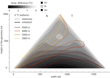
Fig. 3. Difference in the subsurface temperature field for a
sta-tionary simulation compared to model runs initialized with differ-ent surface temperature histories: The 0◦C and−3◦C isotherms for
the different model runs are plotted over the stationary solution de-picted in color.
1300 AD), the Little Ice Age (LIA, ca. 1300–1850 AD), and the subsequent 20th Century warming are typically re-solved in temperature reconstructions (cf. Dahl-Jensen et al., 1998). With increasing spatial and temporal refinement, cli-mate variations become more complex and reconstructions more detailed, particularly towards the present time. This meets our needs since due to the diffusive nature of heat flow a temperature signal entering into the subsurface is damp-ened with depth. That is, the temporal resolution of the surface temperature variations affecting subsurface temper-atures decreases with depth.
We analyze the influence of the above-mentioned periods (Fig. 2) on the present-day subsurface temperature field in-side steep mountains. The effects of temperature variations further back in time or of smaller amplitude are considered negligible. For a detailed description of the most recent tem-perature fluctuations we used measured variations in mean annual air temperatures (MAAT) from a high Alpine station (Jungfraujoch, Switzerland, 3576 m a.s.l.), where air temper-ature data is available back to 1933 AD (Data Source: Me-teoSwiss). The difference in mean temperatures between the periods 1990–1999 AD and 1933–1950 AD amounts to +1◦C for this station. Additionally, we assumed a difference
in air temperature of+0.5◦C between the end of the LIA and
the start of the data recordings, resulting in a total increase of +1.5◦C since 1850 AD (cf. Boehm et al., 2001).
Based on the above described considerations, we explore the effect of the following scenarios of temperature history in order to decide on the initialization procedure (Fig. 2):
temperatures (Patzelt, 1987), followed by a linear in-crease from the time of maximum glaciation (18 ky BP) to the beginning of the Holocene (10 ky BP). For the Holocene no temperature variations were considered. To assess the effect of colder estimates, we additionally used a value of−15◦C (Haeberli et al., 1984).
– HCO (3): During the Holocene Climate Optimum sum-mer temperatures were approx. 1.5–3◦C warmer than
today (Burga, 1991). Mean annual temperatures prob-ably were not as high, but to test the influence of this period we assumed+2◦C.
– Past millennium (4): In contrast to e.g., von Rudloff (1980), newer studies conclude that air tem-peratures in Europe during the MW were probably not warmer than or comparable to today (Hughes and Diaz, 1994; Crowley and Lowery, 2000; Goosse et al., 2006). Yet, to estimate the possible influence of the MW we used 0.5◦C higher surface temperatures than at present.
For the LIA, we assumed temperatures 1.5◦C lower
(Boehm et al., 2001).
– Recent warming: We used a linear temperature increase following the LIA (5) and, in addition, annual MAAT variations taken from Jungfraujoch meteodata (6). Further, to asses the transient response of the subsurface temperature field to future warming, we used a warming sce-nario of the rock surface of +3◦C/100 y. This value has
been calculated as a mean warming of Alpine rock surfaces from 1982–2002 to 2071–2091, based on output from differ-ent Regional Climate Models, differdiffer-ent emission scenarios, downscaling methods, and varying topographic settings by Salzmann et al. (2007). Since no information on the form of the increase (e.g., exponential) was deducted and uncertain-ties are high, we chose a linear increase. Based on this sim-ple scenario, the principal effects of the transient response of bedrock temperatures can be investigated.
4 Transient temperature fields below idealized topography
4.1 Effects of past climatic conditions
If not indicated otherwise, results are discussed and visual-ized for a ridge cross section of 1000 m height with a maxi-mum elevation of 3500 m a.s.l., and a slope angle of 50◦; the
subsurface material is assumed homogenous and isotropic, and no latent heat is considered. Variations from these basic settings are mentioned in the text and indicated in the fig-ures with checkboxes and corresponding abbreviations (i.e., ini for initialized, lh for latent heat considered, and iso for isotropic subsurface conditions).
The stationary temperature field describes the general character of the subsurface temperature pattern of the ridge,
which does not fundamentally differ for temperatures re-sulting from initialized model runs. The latter, however, are lower for the entire thermal field and all GST histories used. 0◦C and
−3◦C-isotherms of temperature fields
ini-tialized with different GST histories are compared to sta-tionary conditions with current GST in Fig. 3: According to the definition of permafrost, the 0◦C isotherm stands for
the schematic permafrost boundary in the idealized mountain ridge, whereas the−3◦C isotherm relates to the temperature
distribution inside the schematic permafrost body. The re-sulting temperature depressions from the last Ice Age (1) is in the range of−0.5◦C for the upper half of the geometry,
and in the range of−2.5◦C for the lower part. When
assum-ing colder GST in the last Ice Age (2) these values amount to−1◦C and−4◦C, respectively. Simulating the GST
vari-ations during the Holocene (4) results in additionally lower temperatures: On the one hand, the LIA (5) is perceivable down to about 250 m depth. On the other hand, deeper parts are modeled colder because (1) and (2) do not consider that present-day GST are somewhat higher than Holocene aver-age. The effect of the HCO (3) is below 0.1◦C for the entire
geometry, and results are therefore not displayed in Fig. 3. Results for GST history (6) do not notably differ from (5) and are not shown, either. Based on the results from (1) to (6), we compiled GST history (7), which accounts for the variations for which a significant influence was shown above. Although we use highly idealized conditions in the experiments, it can be assumed that these are the most important variations that influence the subsurface thermal field in high mountains, be-cause thermal properties and size of the major part of Alpine topography does not essentially differ from the geometries used: We considered the cold temperatures during the last Ice Age (1) and the major fluctuations in the past millennium (4). GST history (7) is used for all subsequent calculations in this study and corresponding temperature fields are referred to as “initialized” or “transient”.
Figure 4 depicts the isotherms of the initialized tempera-ture pattern together with the stationary field for current GST. The initialized temperature field is colder and in the upper-most 100 m the recent warming since the LIA is clearly vis-ible. In the middle part of the warmer side of the ridge, the inclination of the isotherms is reversed. In this part of the ge-ometry, we identify the biggest differences compared to sta-tionary conditions. The absolute temperature difference of a transient to a stationary thermal field for present-day GST is plotted in Fig. 5. Maximum calculated temperature de-pressions in the innermost parts of the geometry are−3◦C,
whereas the temperature depression does not exceed 1◦C in
Fig. 4. The isotherms of a stationary temperature field (thin grey
lines and background colors) compared to an initialized one (tem-perature history (7) from Fig. 2). The transient tem(tem-perature field is shown for simulations both with (solid line) and without (dotted line) considering the effects of latent heat. The porosity was set to 3%.
4.1.1 Topography
For simulations based on conduction only, the elevation of the geometry changes the absolute temperature field but not its pattern. The temperature depressions given above are thus valid for ridge-topographies of any elevation, but the position of the 0◦C isotherm varies (Fig. 5). The
corre-sponding difference in thickness (which we consider verti-cal to the surface) of the “permafrost zone” in the simpli-fied ridge (in brackets because we have not looked at a real situation in nature but at idealized geometries) between sta-tionary and transient results increases for higher mountains with thicker “permafrost”. For the highest example shown in Fig. 5 (4500 m a.s.l.), the difference amounts to more than 100 m. For the lowest example (3000 m a.s.l.) it is in the dimension of decameters.
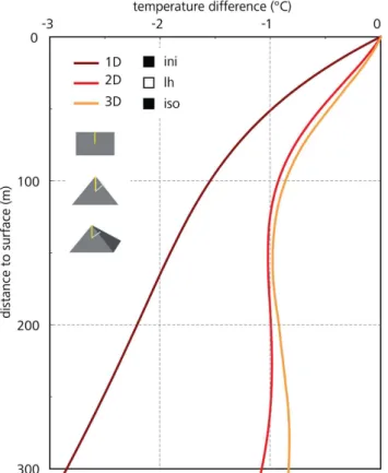
Convex topography accelerates the reaction of the subsur-face temperature to changing sursubsur-face conditions. Firstly and more obviously, the distance a signal has to penetrate to reach the interior of the mountain is shorter than in flat terrain. The steeper the topography, the shorter is this distance. In addi-tion to this effect, the warming signal reaches a point in the interior from more than one side, that is, from two sides in the case of a ridge, and from four sides in a pyramid-like situation. To demonstrate this effect of multi-lateral warm-ing, we compare the temperature depressions in T(z)-profiles in a flat one-dimensional plane, a two-dimensional ridge, and a three-dimensional pyramid (Fig. 6). For the two- and three-dimensional geometries, the profiles are extracted ver-tically from the top of the geometry. The resulting temper-ature depression, however, was not plotted versus the length of the profile, but versus the shortest distance of the profile
Fig. 5. The difference of the stationary solution to an initialized
one (temperature history 7 from Fig. 2) is shown in gray colors. The lines indicate the permafrost boundary for the stationary (dot-ted line) and the transient (solid line) simulation, respectively, for four different maximum elevations of a ridge ranging from 3000 to 4500 m a.s.l. Colors indicate different elevations.
to the surface (i.e., the distance, the signal has to penetrate, cf. schematic plots in Fig. 6). In this way, multi-lateral warm-ing causes the effect shown, and not the fact that the distance to the surface is shorter than the depth of the profile. For the two mountain geometries the modeled temperature depres-sion is roughly half of that for a flat plane in the 200 m clos-est to the surface. For the deeper parts (i.e., 300 m and more), the difference increases and ca. −3◦C for flat terrain
con-trast with ca.−1◦C for two- and three-dimensional mountain
topography. The effect of the three-dimensional compared to the two-dimensional geometry is small for the long time scale of the initialization and the depth range shown. This is due to the fact that the major part of the temperature signal has reached the depths shown in both mountain geometries (cf. also Sect. 4.2 and Fig. 9).
4.1.2 Subsurface properties
Information about subsurface properties of bedrock (such as thermal properties, porosity, and freezing characteristics) is sparse for natural conditions in high mountains. In order to gain confidence in the modeling results, we tested their pos-sible influence in sensitivity studies.
Energy consumption due to latent heat is of minor impor-tance for low porosity material and for the time (i.e., mil-lennia) and depth (i.e., ca. 500 m from the surface) scales considered in the idealized simulations (Fig. 5): subsur-face temperatures are slightly colder compared to simula-tions without latent heat, but differences do not exceed 0.2◦C
Fig. 6. Temperature depression in the subsurface thermal field of
today caused by colder past surface temperatures for one- (flat ter-rain), two- (ridge), and three-dimensional (pyramid) situations. In the two- and three-dimensional situations, profiles are extracted ver-tically from the top of the geometry. Temperature differences are plotted versus the shortest distance to the surface, i.e., the distance the temperature signal penetrated.
time periods (i.e., centuries, see Sect. 4.2.2) or for consider-ably higher porosities. In mountain permafrost areas, high ice contents may be present in the near surface layer, where porosity is often increased due to weathering and fracturing. For example, the ice content of the Schilthorn crest, Switzer-land, is estimated to be roughly 10–20% in the upper me-ters and around 5% in the deeper parts (e.g., Scherler, 2006, Hauck et al., 2008). For this reason, we examined the con-cept of the influence of conduction through an upper layer with a higher ice-content on the transient temperature field below. We added a 15 m thick layer with 20% porosity as a surface layer to the ridge geometry. Yet, no considerable dif-ference to the simulations with homogenous porosity for the entire ridge resulted. However, it must be emphasized at this place that other processes than conduction and phase change are not considered and are likely to play an important role in such a weathered layer (e.g., Scherler, 2006).
Thermal conductivities of bedrock often show large vari-ations due to anisotropy (e.g., in gneiss). Values for the anisotropy factor of crystalline rocks are typically between 1.2 and 2 (Schoen, 1983; Kukkonen and Safanda, 2001). In
Fig. 7. Transient temperature field of an isotropic medium (background colors, gray lines) compared to anisotropic mediums with increased horizontal (anisotropy 1, solid lines) and vertical (anisotropy 2, dotted lines) thermal conductivity, respectively.
order to investigate the anisotropy effect on the temperature field we performed model runs with thermal conductivity in-creased both, horizontally and vertically: In a first run, the thermal conductivity was set to 2 W K−1m−1in x-direction and to 3 W K−1m−1in the perpendicular z-direction direc-tion. For the second run, the vertical and horizontal ther-mal conductivities were swapped (i.e., the anisotropy factor was set to 0.66 in the first and to 1.5 in the second run). An increased horizontal thermal conductivity supports lat-eral heat fluxes and the effect of steep topography, whereas an increased vertical component reduces it. The latter has a bigger effect on the modeled temperatures in the interior of the geometry and increases the effect from past climate conditions: Differences to isotropic conditions amount up to –2◦C for increased vertical thermal conductivity, and 0.5◦C
for increased horizontal conductivity (Fig. 7).
The heat capacity of bedrock typically ranges from about 1.8 to 3×10⁶J kg−1K−1(Cerm´ak and Rybach, 1982). Test runs with varying values result in a maximum difference of less than 1◦C for the inner part of the ridge geometry.
The geothermal heat flux has only a small influence on the stationary subsurface temperature field inside steep moun-tain peaks (Noetzli et al., 2007b). This is also true for the transient calculations presented here: Resulting temperature depressions from simulations with a zero heat flux lower boundary condition were assessed to differ less than 0.2◦C.
Further, we tested the influence of radiogenetic heat produc-tion. Values for rock are given between 0.5 and 6µW m−3
(Kohl, 1999). We used a medium value of 3µW m−3 for
a test run. Maximum differences to results without heat production were assessed to be below 0.5◦C for the entire
Fig. 8. The temperature difference between the current transient
temperature field and a 200-year scenario simulation is displayed in gray shadings. The warming has penetrated to ca. 250 m depth. The evolution of the 0◦C isotherms for a 200-year scenario is
plot-ted for different elevations of the ridge. Colors indicate different elevations, whereas the dotted patterns represent the situation today (solid lines), in 100 years (dashed lines), and in 200 years (dotted lines).
4.2 Effects of future warming
The effect of a linear temperature rise at the surface of +3◦C/100 y during 200 years on the subsurface thermal field
in steep topography has been shown in numerical experi-ments by Noetzli et al. (2007b). The results showed that the warming has penetrated to a depth of approximately 250 m after 200 years, but only about 50% of the temperature change has reached a depth of more than 100 m. Tempera-tures at greater depth than ca. 250 m still remain unchanged after 200 years. Further, a retarding influence of latent heat was demonstrated. In this study, we look at the idealized re-sponse of thermal fields in high mountains to possible future temperature changes that are caused by elevation, geometry, and subsurface conditions.
4.2.1 Topography
In Fig. 8, the state of the schematic permafrost body inside the ridge geometry is displayed for the situation after follow-ing the linear temperature scenario for 200 years and differ-ent elevations. The position of the 0◦C isotherm at 250 m or
closer to the surface changes drastically and is bent towards the top. On the warmer side of the geometry, the isotherms first change to run more or less parallel to the surface and then move rather uniformly towards the colder side. For all elevations, no below zero temperatures, or “permafrost”, re-main at the surface on the southern slope of the idealized geometry. Nevertheless, a significant “permafrost body” re-mains below the surface for a long time, especially for higher elevations. For lower elevations a “permafrost body” remains only on the colder side.
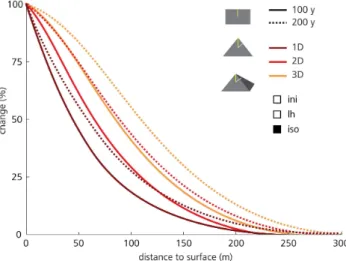
Fig. 9. Percent of a temperature signal at the surface that has penetrated to depth: This effect is shown for a one- (flat terrain), two- (ridge), and three-dimensional (pyramid) situation after 100 (solid lines) and 200 years (dotted lines). In the two- and three-dimensional situations values are plotted versus the shortest dis-tance to the surface.
The above-described (Sect. 4.1.1) effect of multi-lateral warming is also significant for shorter time periods. Figure 9 displays the percentage of a surface temperature signal that has reached a certain depth after 100 and 200 years. For ex-ample, 50% of the temperature signal has reached a depth of about 60 m after 200 years in a one-dimensional vertical simulation. In the two-dimensional situation, 50% of the sig-nal has already penetrated to about 90 m, and in the three-dimensional situation to ca. 115 m. In the same way as in Fig. 6, values for the two- and three-dimensional geometries are plotted versus the shortest distance to the surface, rather than versus the length of the profile.
4.2.2 Subsurface conditions
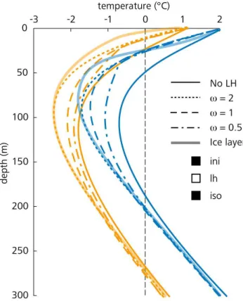
The effect of latent heat on the temperature fields subject to the idealized future scenario is illustrated in Fig. 10. It leads to a considerably slower decrease of the zone with below zero temperatures. With varying freezing range (parameterw) the
size of this zone does not change significantly, but the tem-perature distribution in it does. A smaller value ofw(i.e.,
a smaller freezing range and a steeper unfrozen water con-tent curve) keeps the thermal field for a longer time period in the temperature ranges little below the melting point. This leads to more homogeneous temperature fields than when modeled with a larger value of w. When looking at
Fig. 10. The permafrost body in a ridge calculated for a 200-year
scenario is displayed for simulations with and without considering the effects of latent heat and a porosity of 3%. Additionally, differ-ent values of the parameterw, which describes the unfrozen water
content curve, have been considered. Black lines represent the mod-eled 0◦C isotherm, i.e., the remaining permafrost body; blue, red, and yellow lines the−1,−2, and−3◦C isotherms.
This points to subsurface material with a small freezing in-terval and a low value ofw. The observed higher ice-content
in the near-surface layer (cf. Sect. 4.1.2) can act as a buffer to temperature changes at the surface and further delay the short-term reaction of the subsurface temperature field, when looking at time scales of the next 1–2 centuries (Fig. 11).
5 Application to the topographic setting of the Matterhorn
The Matterhorn (4478 m a.s.l.) in Switzerland is probably the most prominent mountain peak in the European Alps. Its distinctive topography resembles a pyramid of about 1500 m height with faces exposed to the four main orientations. Slope angles are >45◦C for most parts and only isolated
or thin patches of snow persist on the rock. With its ex-treme three-dimensional geometry, the Matterhorn consti-tutes a prime example for an application of the presented modeling approach to real topography. The application of the modeling procedure to the Matterhorn topography is seen as a step towards more natural conditions. Further, it is helpful to intuitively understand the dimensions of changes shown in the results from idealized geometries. Based on the ex-perience gained with the previous experiments and the val-idations conducted (see Sect. 3.2), the modeling procedure allows to describe the principal pattern of the subsurface tem-perature and permafrost distribution inside the mountain and how they may evolve in the future. However, results need to be interpreted with great care, especially where a consid-erable snow or glacier cover influences the ground temper-atures (cf. Sect. 6). For a detailed description and the re-quirement to accurately model subsurface temperatures, the modeling has to be calibrated and tested against measured
Fig. 11. T(z)-profiles of two synthetic boreholes vertical to the
slope in the middle and the lower part of the North side of a ridge (cf. Fig. 10) illustrate the effect of latent heat and the freezing range
w. In addition, thick bright lines display the profile of a simulation
with a 20 m ice-rich layer at the surface.
data from the Matterhorn. Several measurement sites have recently been instrumented and corresponding datasets will be available soon. Temperature data are measured on the H¨ornli Ridge (NE ridge: two 60 m boreholes close to the H¨ornlih¨utte that are monitored within the PERMOS project (PERMOS, 2007), and extensive thermal and geotechnical measurements at the 2003 rock fall scar within the project PermaSense; Hasler et al., 2008) and the Lion Ridge (SW ridge, Carell Hut, near surface temperature measurements in the scope of the project PermaDataRock (Pogliotti, 2006).
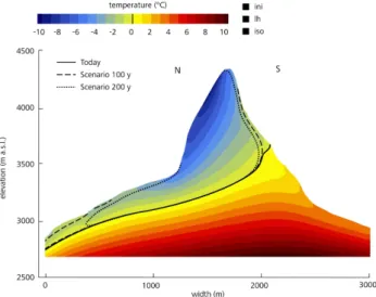
Fig. 12. North-south cross section of the Matterhorn (4478 m a.s.l.)
and modeled subsurface temperature field for today (i.e., the mean of the period 1990–1999 AD). The temperature field was computed transient, three-dimensional, isotropic, and with 3% subsurface ice in the frozen parts. The black lines represent the 0◦C isotherms for
today (solid line), in 100 years (dashed line), and in 200 years (dot-ted line). We assumed a linear warming scenario of+3◦C/100 y.
DHM 25 reproduced by permission of swisstopo (BA091262).
east Alpine Dent-Blanche nappe. We set a thermal con-ductivity of 2.5 W m−1K−1, a volumetric heat capacity of 2.2×10⁶J m−3K−1, a porosity of 3%, and
w=2 (cf. Table 1).
Boundary conditions and time steps were the same as in the simulations presented above, and anisotropy was not consid-ered.
A north-south cross section through the resulting subsur-face temperature field for current conditions and the warm-ing scenario for 200 years is given in Fig. 12. The ex-treme pyramid-like geometry of the Matterhorn leads to a strongly three-dimensional subsurface temperature field, which is characterized by steeply inclined isotherms, a strong heat flux from the south to the north, and a smaller heat flux from the east to the west face. For present-day conditions and all the simplifications assumed for the simulation, the entire mountain is within permafrost, except for the lower parts of the South side. Additionally considering the ideal-ized scenario, surface temperatures on nearly the entire South side would be positive after 200 years. On the North side, the 0◦C isotherm at the surface would have risen to an
el-evation of about 3500 m a.s.l. The calculated scenario indi-cates further that possibly substantial permafrost can remain a few decameters below the surface both, on the south and the north side. Temperatures of the remaining sketched per-mafrost body are warming and the extent of so-called warm permafrost (i.e., about−2 to 0◦C) would significantly
in-crease in volume as well as in vertical extent (Fig. 13).
Fig. 13. Modeled temperature range of−2 to 0◦C in a north-south
cross section of the Matterhorn for today (gray), in 100 years (light red), and in 200 years (red). We assumed a linear warming scenario of+3◦C/100 y. DHM 25 reproduced by permission of swisstopo
(BA091262).
6 Discussion
With the numerical experiments based on simplified moun-tain topographies having idealized surface and subsurface conditions we analyzed the influence of combined transient and three-dimensional topography effects on the subsurface temperature field in mountain topographies. For the interpre-tation of the results, a number of uncertainties and limiinterpre-tations of the modeling approach used are important and the simpli-fications made have to be kept in mind.
Instrumental records of climate parameters are typically available for the past ca. 100 years. Reconstructions of pre-industrial climate rely on proxy data and are subject to a great number of uncertainties, which may be even larger than the influence a certain time period has on the subsurface tem-peratures. In general, climate reconstruction studies agree well on the shape of the climate fluctuations, whereas the absolute amplitude of the temperature variations ranges sig-nificantly (Esper et al., 2005). Further, we assumed that changes in GST closely follow air temperatures. Salzmann et al. (2007) demonstrated a considerable influence of topog-raphy on the reaction of surface temperatures in steep rock to changing atmospheric conditions. The dimensions of the GST changes, however, are not influenced, and in view of the above-mentioned uncertainties of the reconstructed am-plitudes of temperature variations, we consider this effect to be less important for this study.
glacier-covered areas are likely smaller than in rock directly exposed to the atmosphere during the entire simulation pe-riod. This is likely important, for example, for the lower parts of the Matterhorn. In these parts, the temperature field shown in Figs. 12 and 13 has to be interpreted with great care and may considerably deviate in nature. The negligence of the snow cover is a further significant limitation of the model-ing approach: Snow cover affects the energy balance at the ground surface by increasing albedo, consuming melt energy, and insulating the ground surface from atmospheric condi-tions. Snow that remains in steep bedrock can have both, a cooling and a warming effect. For steep rock slopes, how-ever, these effects have not yet been investigated or quan-tified in detail and results from more gentle terrain cannot be directly transferred to steeper areas (Gruber and Haeberli, 2007). In view of applying the model to less inclined slopes, the influence of a snow cover will have to be included in the model.
In terms of subsurface characteristics, errors induced by uncertain assumptions of thermal conductivity, heat capac-ity, and heat production increase with depth and length of the simulation, whereas errors caused by uncertainties in sub-surface ice decrease. Information on the amount and freez-ing characteristics of subsurface ice in bedrock is required to improve realistic modeling, but is still scarce. The joint in-terpretation of numerical model results with data from geo-physical monitoring (e.g., electrical resistivity tomography, ERT) has been successfully realized for a first case study of the Schilthorn crest in the Swiss Alps (Noetzli et al., 2008), and information gained in this way may help to improve the representation of the subsurface in the model.
Neglecting water circulation along the joint systems of bedrock is another limitation of the approach used. Advec-tive heat transfer along clefts can contribute, for example, to subsurface heat transfer and lead to thaw corridors in per-mafrost, which substantially modify a purely conductive sys-tem (Gruber et al., 2004a; Gruber and Haeberli, 2007). First applications of geophysical monitoring in solid rock walls re-cently identified thawed cleft systems influenced by moving water (Krautblatter and Hauck, 2007). Process understand-ing of advective heat transfer processes in steep bedrock per-mafrost, however, is limited. But such processes are expected to be important especially in the upper decameters.
We assumed a linear temperature rise of+3◦C in 100 y for
the calculations of the idealized response of the temperature fields to future changes. An exponential temperature rise as generally proposed for climate change scenarios may slow down the temperature changes calculated. Yet, the temper-ature increase assumed represents a calculated mean change in GST of Alpine bedrock (Salzmann et al., 2007) and is at the lower range of the scenarios presented for air temperature change by IPCC (2007), where a double temperature raise is not considered unrealistic or extreme for the Alps. The general pattern of a future temperature field that increasingly deviates from steady state conditions and experiences major
changes in heat fluxes in the upper ca. 100–200 meters is not affected by these uncertainties.
Because of its temperature range, the acceleration of sub-surface temperature changes through multi-lateral warming, and the virtual decoupling from the geothermal heat flux, bedrock permafrost in steep high mountain areas is partic-ularly sensitive to climate change. The simulations of pos-sible future subsurface temperatures with idealized moun-tain topographies point to long lasting and deep-reaching changes in the subsurface thermal field. For all settings in the experiments, only very little “permafrost” remains at the surface on south-facing Alpine rock slopes in 200 years. Simulated 0◦C-isotherms are about to change to a
surface-parallel course in the top parts of the mountain geometries and then move rather uniformly towards the interior. In terms of temperature-related instabilities such a thawing and hori-zontally migrating permafrost table may be delicate: rock volumes with temperatures close to the melting point, possi-bly containing critical ice-water-rock mixtures, increase and may extend over large vertical distances up to entire moun-tain flanks.
Although our experiments were conducted for strongly idealized conditions, the general pattern and the principal ef-fects shown in this paper can be transferred to real topogra-phies, but keeping in mind the above mentioned uncertainties and the fact that the situation in nature is more complicated and additional processes may be important. For the idealized and simplified present-day temperature field of the Matter-horn, for example, warm permafrost is indicated in the mid-dle part of the South side. In these areas, rock fall events actually have been observed in recent years (2003 and 2006). Looking at the scenario sketched, the zone having temper-ature little below the freezing point extends over the entire south face and, in addition, over large parts of the north face. Although the modeled temperature field can only be inter-preted as a very first approximation to the actual pattern in the Matterhorn, this scenario describes how the surface tem-perature field may develop in view of future changes in at-mospheric conditions.
7 Conclusions and perspectives
The results of the simulations performed with idealized test cases of steep mountain topography lead to the following conclusions:
The main variations in surface temperatures that influence present-day subsurface temperatures in Alpine permafrost are the last glacial period and the major temperature varia-tions in the past millennium.
a distance of 500 m from the surface and for the idealized model settings.
Transient effects likely become even more important for temperature fields influenced by future warming. Model ex-periments point to temperature fields that are characterized by long-term and deep reaching perturbations and by tem-perature patterns that strongly deviate from stationary condi-tions.
Two- and three-dimensional topography significantly ac-celerates the pace of a surface temperature signal entering into the subsurface. Together with the fast and unfiltered re-action of its surface to changes in atmospheric conditions and the low ice content, this makes bedrock permafrost in high mountains particularly sensitive to changes.
For the time (20 kyr) and depth (ca. 500 m) scales consid-ered, the influence of latent heat on the temperature depres-sions caused by past GST variations is small in low porosity rock. In view of other sources of uncertainties (e.g., tem-perature reconstructions) this effect is not considered of ma-jor importance. In connection with possible future warming, however, latent heat effects considerably modify the pace of permafrost degradation and the pattern of the subsurface tem-perature field.
Temperatures of the schematic permafrost body in the ge-ometries are rising when applying the future scenarios, and the extent of “warm permafrost” significantly increases in volume as well as in vertical extent
The distribution and extent of temperatures little below the melting point in a warming subsurface temperature field is significantly influenced by the freezing characteristics of the subsurface material. A small freezing range leads to more homogenous temperature fields and T(z) profiles with small temperature gradients.
The investigation of mountain permafrost by transient three-dimensional modeling has only been used for a few case studies of real mountain topography so far. It bears po-tential for various applications that require knowledge of cur-rent and future thermal conditions of mountain permafrost, for instance, the reanalysis of the thermal conditions in rock fall starting zones located in permafrost areas, the improved interpretation of T(z) profiles measured in boreholes, and the assessment of thermal conditions and their evolution in rock below infrastructure. The limitations and uncertainties discussed above call for improved knowledge of subsurface properties in bedrock permafrost, as well as for enhanced validation and modeling practices. A promising approach may be the combination of numerical modeling together with measurements and interpretation of field data. For example, the representation of the subsurface physical properties in the model can be improved by incorporating subsurface informa-tion (e.g., geological structures, water/ice content) detected by geophysical surveys. Further, process understanding and incorporation of advective heat transfer and snow remaining in steep rock will be important for a realistic modeling of subsurface temperature fields.
Acknowledgements. This study was supported by the Swiss
National Science Foundation, as part of the NF 20-10796./1 project “Frozen rock walls and climate change: transient 3-dimensional investigation of permafrost degradation”. Special thanks go to Sven Friedel for support with the COMSOL software and for providing an import routine for DEMs. Fruitful discussions with W. Haeberli and M. Hoelzle (University of Zurich, Switzerland) as well as with T. Kohl (Geowatt AG, Zurich, Switzerland) were valuably contributed to this study. Careful and constructive comments by the two reviewers helped to improve the paper.
Edited by: A. K¨a¨ab
References
Anderson, D. M. and Tice, A. R.: Predicting unfrozen water con-tents in frozen soils from surface area measurements, Highway Research Record, 393, 12–18, 1972.
Beltrami, H.: On the relationship between ground temperature his-tories and meteorological records: A report on the Pomquet Sta-tion, Global Plaint. Change, 29, 327–348, 2001.
Beltrami, H., Ferguson, G., and Harris, R. N.: Long-term tracking of climate change by underground temperatures, Geophys. Res. Lett., 32, L19707, doi:10.1029/2005GL023714, 2005.
Beniston, M., Diaz, H. F., and Bradley, R. S.: Climatic change at high elevation sites: An overview, Clim. Change, 36, 233–251, 1997.
Beniston, M.: Mountain climates and climate change: An overview of processes focusing on the European Alps, Pure Appl. Geo-phys., 162, 1587–1606, 2005.
Birch, F.: The effects of Pleistocene climatic variations upon geothermal gradients, Am. J. Sci., 246, 729–760, 1948. Boehm, R., Auer, I., Brunetti, M., Maugeri, M., Nanni, T., and
Schoener, W.: Regional temperature variability in the European Alps: 1760–1998 from homogenized instrumental time series, Int. J. Climatol., 21, 1779–1801, 2001.
Brown, R. J. E. and P´ew´e, T. L.: Distribution of permafrost in north america and its relationship to the environment, a review 1963– 1973, 2nd International Conference on Permafrost. Proceedings, Yakutsk, USSR, 1973, 71–100, 1973.
Burga, C.: Vegetation history and paleoclimatology of the middle Holocene: Pollen analysis of Alpine peat bog sediments, cov-ered formerly by the Rutor Glacier, 2510 m (Aosta Valley, Italy), Global Ecol. Biogeogr., 1, 143–150, 1991.
Carslaw, H. S. and Jaeger, J. C.: Conduction of heat in solids, Oxford science publications, Clarendon Press, Oxford, 510 pp., 1959.
Casty, C., Wanner, H., Luterbacher, L., Esper, J., and Boehm, R.: Temperature and precipitation variability in the European Alps since 1500, Int. J. Climatol., 25, 1855–1880, 2005.
Cerm´ak, V. and Rybach, L.: Thermal conductivity and specific heat of minerals and rocks, in: Landolt-b¨ornstein Zahlenwerte und Funktionen aus Naturwissenschaften und Technik, neue Serie, physikalische Eigenschaften der Gesteine (v/1a), edited by: An-geneister, G., Springer, Berlin, 305–343, 1982.
Crowley, T. J. and Lowery, T. S.: How warm was the Medieval Warm Period? Ambio, 29, 51–54, 2000.
directly from the Greenland Ice Sheet, Science, 282, 268–271, 1998.
Davies, M. C. R., Hamza, O., and Harris, C.: The effect of rise in mean annual temperature on the stability of rock slopes contain-ing ice-filled discontinuities, Permafrost Periglac., 12, 137–144, 2001.
Esper, J., Wilson, R. J. S., Frank, D. C., Moberg, A., Wanner, H., and Luterbacher, J.: Climate: Past ranges and future changes, Quarternary Sci. Rev., 24, 2164–2166, 2005.
Goosse, H., Arzel, O., Luterbacher, J., Mann, M. E., Renssen, H., Riedwyl, N., Timmermann, A., Xoplaki, E., and Wanner, H.: The origin of the European “Medieval Warm Period”, Clim. Past, 2, 99–113, 2006,
http://www.clim-past.net/2/99/2006/.
Gruber, S., Hoelzle, M., and Haeberli, W.: Permafrost thaw and destabilization of Alpine rock walls in the hot summer of 2003, Geophys. Res. Lett., 31, L13504, doi:10.1029/2004GL0250051, 2004a.
Gruber, S., Hoelzle, M., and Haeberli, W.: Rock wall temperatures in the Alps: Modeling their topographic distribution and regional differences, Permafrost Periglac., 15, 299–307, 2004b.
Gruber, S., King, L., Kohl, T., Herz, T., Haeberli, W., and Hoelzle, M.: Interpretation of geothermal profiles perturbed by topog-raphy: The Alpine permafrost boreholes at Stockhorn Plateau, Switzerland, Permafrost Periglac., 15, 349–357, 2004c. Gruber, S.: Mountain permafrost: Transient spatial modelling,
model verification and the use of remote sensing, PhD Thesis, Department of Geography, University of Zurich, Zurich, 2005. Gruber, S., and Haeberli, W.: Permafrost in steep bedrock
slopes and its temperature-related destabilization fol-lowing climate change, J. Geophys. Res., 112, F02S18, doi:10.1029/2006JF000547, 2007.
Haeberli, W.: Permafrost-glacier relationships in the Swiss Alps – today and in the past, 4th International Conference on Per-mafrost. Proceedings, Fairbanks, Alaska, 1983, 415–420, Haeberli, W., Rellstab, W., and Harrison, W. D.: Geothermal effects
of 18 ka BP ice conditions in the Swiss Plateau, Ann. Glaciol., 5, 56–60, 1984.
Haeberli, W.: Construction, environmental problems and natural hazards in periglacial mountain belts, Permafrost Periglac., 3, 111–124, 1992.
Haeberli, W., Wegmann, M., and Vonder M¨uhll, D.: Slope stability problems related to glacier shrinkage and permafrost degradation in the Alps, Eclogae Geol. Helv., 90, 407–414, 1997.
Haeberli, W. and Beniston, M.: Climate change and its impacts on glaciers and permafrost in the Alps, in: Ambio – a journal of the human environment, edited by: Rapp, A., and Kessler, E., 4, The Royal Swedish Academy of Sciences, 258–265, 1998.
Harris, C., Davies, M. C. R., and Etzelm¨uller, B.: The assessment of potential geotechnical hazards associated with mountain per-mafrost in a warming global climate, Perper-mafrost Periglac., 12, 145–156, 2001.
Hasler, A., Talzi, I., Beutel, J., Tschudin, C., and Gruber, S.: Wire-less sensor networks in permafrost research: Concept, require-ments, implementation, and challenges, 9th International Con-ference on Permafrost, Fairbanks, US, 669–674, 2008.
Hauck, C., Bach, M., and Hilbich, C.: A 4-phase model to quan-tify subsurface ice and water content in permafrost regions based on geophysical datasets, 9th International Conference on
Per-mafrost, Fairbanks, US, 675–680, 2008.
Huang, S., Pollak, H. N., and Shen, P. Y.: Temperature trends over the last five centuries reconstructed from borehole temperatures, Nature, 403, 756–758, 2000.
Hughes, M. K., and Diaz, H. F.: Was there a “Medieval Warm Pe-riod”, and if so, where and when?, Clim. Change, 26, 109–142, 1994.
IPCC: Climate change 2007: The physical science basis. Contribu-tion of working group I to the fourth assessment report of the In-tergovernmental Panel on Climate Change, edited by: Solomon, S., Qin, D., Manning, M., Chen, Z., Marquis, M., Averyt, K. B., Tignor, M., and Miller, H. L., Cambridge University Press, Cambridge, United Kingdom and New York, 996 pp., 2007. Isaksen, K., Vonder M¨uhll, D., Gubler, H., Kohl, T., and Sollid,
J. L.: Ground surface temperature reconstruction based on data from a deep borehole in permafrost at Janssonhaugen, Svalbard, Ann. Glaciol., 31, 287–294, 2000.
Isaksen, K., Sollid, J. L., Holmlund, P., and Harris, C.: Recent warming of mountain permafrost in Svalbard and Scandinavia, J. Geophys. Res., 112, F02S04, doi:10.1029/2006JF000522, 2007. Jones, P. D., Briffa, K. R., Barnett, T. P., and Tett, S. F. B.: High-resolution paleoclimatic records for the last millennium: Inter-pretation, integration, and comparison with general circulation model control-run temperatures, Holocene, 8, 455–471, 1998. Jones, P. D. and Mann, M. E.: Climate over past millennia, Rev.
Geophys., 42, RG2002, doi:2010.1025/2003RG000143, 2004. Kohl, T.: Transient thermal effects at complex topographies,
Tectonophysics, 306, 311–324, 1999.
Kohl, T., Signorelli, S., and Rybach, L.: Three-dimensional (3-D) thermal investigation below high Alpine topography, Phys. Earth Plaint. In., 126, 195–210, 2001.
Kohl, T. and Gruber, S.: Evidence of paleaotemperature signals in mountain permafrost areas, 8th International Conference on Per-mafrost, Extended Abstracts, Z¨urich, 83–84, 2003.
Krautblatter, M. and Hauck, C.: Electrical resistivity tomography monitoring of permafrost in solid rock walls, J. Geophys. Res., 112, F02S20, doi:10.1029/2006JF000546, 2007.
Kukkonen, I. T. and Safanda, J.: Numerical modelling of permafrost in bedrock in northern Fennoscandia during the Holocene, Glob. Plaint. Change, 29, 259–273, 2001.
Lachenbruch, A. H. and Marshall, B. V.: Changing climate: Geothermal evidence from permafrost in the alaskan arctic, Sci-ence, 234, 689–696, 1986.
L¨uthi, M. and Funk, M.: Modelling heat flow in a cold, high-altitude glacier: Interpretation of measurements from Colle Gnifetti, Swiss Alps, J. Glaciol., 47, 314–324, 2001.
Lunardini, V. J.: Climatic warming and the degradation of warm permafrost, Permafrost Periglac., 7, 311–320, 1996.
Luterbacher, J., Dietrich, D., Xoplaxi, E., Grosjean, M., and Wan-ner, H.: European seasonal and annual temperature variability, trends and extremes since 1500, Science, 303, 1499–1503, 2004. Medici, F. and Rybach, L.: Geothermal map of Switzerland 1995 (heat flow density), G´eophysique 30, Schweizerische Geo-physikalische Kommission, 1995.
Mottaghy, D. and Rath, V.: Latent heat effects in subsurface heat transport modeling and their impact on paleotemperature recon-structions, Geophys. J. Int., 164, 236–245, 2006.
University of Zurich, Zurich, 150 pp., 2008.
Noetzli, J., Hoelzle, M., and Haeberli, W.: Mountain permafrost and recent Alpine rock-fall events: A GIS-based approach to determine critical factors, 8th International Conference on Per-mafrost, Proceedings, Z¨urich, 827–832, 2003.
Noetzli, J., Gruber, S., and Friedel, S.: Modeling transient per-mafrost temperatures below steep Alpine topography, COMSOL User Conference, Grenoble, 139–143, 2007a.
Noetzli, J., Gruber, S., Kohl, T., Salzmann, N., and Haeberli, W.: Three-dimensional distribution and evolution of permafrost tem-peratures in idealized high-mountain topography, J. Geophys. Res., 112, F02S13, doi:10.1029/2006JF000545, 2007b. Noetzli, J., Hilbich, C., Hauck, C., Hoelzle, M., and Gruber, S.:
Comparison of simulated 2D temperature profiles with time-lapse electrical resistivity data at the Schilthorn crest, Switzer-land., 9th International Conference on Permafrost, Fairbanks, US, 2008, 1293–1298.
Patzelt, G.: Neue Ergebnisse der Sp¨at- und Postglazialforschu-ung in Tirol, in: Jahresbericht, ¨Osterreichische Geographische Gesellschaft, Zweigverein Innsbruck, 11–18, 1987.
PERMOS: Permafrost in Switzerland 2002/2003 and 2003/2004, Glaciological report (Permafrost) no. 4/5 of the Cryospheric Commission of the Swiss Academy of Sciences (SCNAT) and Department of Geography, University of Zurich, edited by: Von-der Muehll, D., Noetzli, J., Roer, I., Makowski, K., and Delaloye, R., 104 pp., 2007.
Petit, J. R., Jouzel, J., Raynnaud, D., Barkov, N. I., Barnola, J.-M., Basile, I., Bender, M., Chappellaz, J., Davis, M., Delaygue, G., Delmotte, M., Kotlyakov, V. M., Legrand, M., Lipenkov, V. Y., Lorius, C., P´epin, L., Ritz, C., Saltzman, E., and Stievenard, M.: Climate and atmospheric history of the past 420 000 years from the Vostok ice core, Antarctica, Nature, 399, 429–436, 1999. Pfister, C.: Wetternachhersage, Haupt, Bern, 304 pp., 1999. Pogliotti, P.: Analisi morfostrutturale e caratterizzazione termica
di ammassi rocciosi recentemente deglaciati. MSc Thesis, Heart Science Department, University of Turin, Turin, 191 pp., 2006. Pollak, H. N., Huang, S., and Shen, P. Y.: Climate change record
in subsurface temperatures: A global perspective, Science, 282, 279–281, 1998.
Pollak, H. N. and Huang, J.: Climate reconstruction from subsur-face temperatures, Ann. Rev. Earth Plaint. Sci., 28, 339–365, 2000.
Romanovsky, V. E. and Osterkamp, T. E.: Effects of unfrozen wa-ter on heat and mass transport processes in the active layer and permafrost, Permafrost Periglac., 11, 219–239, 2000.
Romanovsky, V. E., Gruber, S., Instanes, A., Jin, H., Marchenko, S. S., Smith, S. L., Trombotto, D., and Walter, K. M.: Frozen ground, in: Global outlook for ice and snow, edited by: UNEP, UNEP/GRID-Arendal, Norway, 182–200, 2007.
Safanda, J.: Ground surface temperature as a function of slope angle and slope orientation and its effect on the subsurface temperature field, Tectonophysics, 306, 367–375, 1999.
Safanda, J. and Rajver, D.: Signature of the last ice age in the present subsurface temperatures in the Czech Republic and Slovenia, Glob. Plaint. Change, 29, 241–257, 2001.
Salzmann, N., Noetzli, J., Gruber, S., Hauck, C., and Haeberli, W.: RCM-based ground temperature scenarios in high-mountain to-pography and their uncertainty ranges, J. Geophys. Res., 112, F02S12, doi:10.1029/2006JF000527, 2007.
Scherler, M.: Messung und Modellierung konvektiver W¨armetransportprozesse in der Auftauschicht von Gebirgsper-mafrost am Beispiel des Schilthorns, Department of Geography, University of Zurich, Zurich, 94 pp., 2006.
Schoen, J.: Petrophysik, Ferdinand Enke, Stuttgart, 1983.
Stocker-Mittaz, C.: Permafrost distribution modeling based on en-ergy balance data. PhD-Thesis, Department of Geography, Uni-versity of Zurich, Zurich, 122 pp., 2002.
Suter, S.: Cold firn and ice in the monte rosa and mont blanc areas: spatial occurrence, surface energy balance and climatic evidence, 172, Versuchsanstalt f¨ur Wasserbau, Hydrologie und Glaziologie der ETH Z¨urich, ETH Z¨urich, Z¨urich, 188 pp., 2002.
Von Rudloff, H.: Das Klima – Entwicklung in den letzten Jahrhun-derten im mitteleurop¨aischen Raume (mit einem R¨uckblick auf die postglaziale Periode), in: Das Klima – Analysen und Mod-elle, Geschichte und Zukunft, edited by: Oeschger, H., Messerli, B., and Silvar, M., Springer, Berlin, 125–148, 1980.
Washburn, A. L.: Geocryology – a survey of periglacial processes and environments, edited by: Quartenary Research Center, U. o. W., Edward Arnold Ltd., London, 406 pp., 1979.
Wegmann, M.: Frostdynamik in hochAlpinen Felsw¨anden am Beispiel der Region Jungfraujoch-Aletsch, 161, Versuchsanstalt f¨ur Wasserbau, Hydrologie und Glaziologie der ETH Z¨urich, ETH Z¨urich, Z¨urich, 143 pp., 1998.
Wegmann, M., Gudmundsson, G. H., and Haeberli, W.: Permafrost changes in rock walls and the retreat of Alpine glaciers: A ther-mal modelling approach, Permafrost Periglac., 9, 23–33, 1998. Williams, P. J. and Smith, M. W.: The frozen earth, 1 ed., Studies