Numerical Analysis on Aerodynamic Behavior of a Hemispherical Structure under Different Wind Loading

Numerical Analysis on Aerodynamic Behavior of a Hemispherical

Structure under Different Wind Loading

R. Verma*, V. K. Patel** , A. Pal*

*(Aerial Delivery Research & Development Establishment, DRDO, Agra-282001, India)

** (Motilal Nehru National Institute of Technology Allahabad-211004, India)

ABSTRACT

Light weight and adaptability in structures have attracted researchers towards the development of inflatable structures. These light weighted inflatable structures are used as emergency shelters, as a decoy and also as a permanent building. Earlier reports shows many cases in which these light weight structure have collapsed due to adverse wind conditions. This damage caused to these structures may be attributed to its poor wind resistance design conditions. Also, due to the uncertainties, there is limited and very few information representing the aerodynamic behaviour of the wind over hemispherical dome structures. An attempt is herewith made to find out the aerodynamic behaviour of the wind passing through a hemispherical shaped structure. CFD software FLUENT has been used to perform the analysis of a dome model in Indian wind conditions. Before study, the CFD code has been validated against experimental data available in literature. It is found that the realizable k-ε turbulent model shows good agreement with experimental data. The value of drag coefficient (Cd) has been

calculated by using frontal area of the structure and it is found out to be 0.32. The results with different wind conditions obtained by CFD shows that the increase in turbulent intensity in the flow field highly influences the drag force and it increase approximately 14% for a highly turbulent wind condition.

Keywords:

I.

INTRODUCTION

Rectangular and cubic section structures are most commonly designed and are found in bulk such

as masts, towers chimneys etc. But now a day’s

engineering focuses on curved surfaces as they provide economical ways of roofing large areas. Moreover, these curved surface domes are capable of enclosing maximum amount of space with minimum surface area. Reports show that these hemispherical structure collapses under strong wind conditions as wind load forms a major proportion of the total load acting on the structure. Thus, the distribution of the pressure must be analyzed and taken into consideration.

Analysis of the velocity comes into picture as it gives us the information of the separation point as well as the development of wake region behind the curved shape structure. In addition, the turbulence intensity forms a major part for the study. It provides us with the information for the location allocation of the nearby surrounding structures. Toy et al. [1], Taylor [2] and many more have enriched the literature by their studies on the characteristics of the dome structures. They performed various wind tunnel experiments and conclude the worthwhile results.

Toy et al. [1] studied the flow past a hemispherical dome immersed in two turbulent boundary layers of different velocity profiles and turbulence intensity. They plotted the Pressure distributions on the surface of the dome along with

mean velocity and turbulence intensity profiles measured in the near wake regions using hot-wire anemometers. They found that the separation point move in the downstream with the increase in turbulence intensity. They also confirmed that the width of the shear layer and the maximum turbulence intensity are dependent on the turbulence in the approaching boundary layer.

Taylor [2] also performed a wind tunnel experiment similar to Toy et al. [1] and measured the surface pressure on the hemispherical dome in the two natural boundary layer models. He found that the pressure measurements become relatively insensitive to the Reynolds number (above 1.7×105) for turbulence intensity greater than 15% of natural wind. Below this transition Reynolds number the average pressure over an area of the hemispherical domes surface decreased the peak pressure coefficients over that area and this is more significant for the lower height and diameter ratios than for h/D= 1.

Now a day’s CFD has been growing as an

efficient tool for the study of fluid flow behavior. Literature shows a limited work on the computational study for the aerodynamic behavior over the hemispherical surfaces. Hence, an effort is made to study the characteristics over the dome structure with the help of computation method through CFD Code FLUENT [3]. Also, the size and setup makes experiment much expensive. CFD is being increasingly used as an efficient and cost effective tool. It provides us with the methods to

study the distribution of pressure. The distribution of pressure plays an important role in the stability of the dome structure.

Cheng and Fu [4] performed experiments and investigated the distribution of the pressure for various Reynolds number. In their results with smooth flow, they found that the transition of separation flow occurs between Re=1.8×105 to 3.0×105 and pressure distributions become comparatively stable after Re>3.0×105. However, in their study with turbulent flow, the separation flow occurs at lower Reynolds number, Re<1.1×105, whereas the pressure distributions turn into independent of Reynolds number at Re=2.0×105.

In the present study, the results by Cheng and Fu [4] have been taken as reference and it is used for the validation of CFD code. Further, this validated code has been used for further studies with different wind conditions.

II.

MATHEMATICAL

MODEL

CFD Code fluent has been used to study the flow characteristics. The governing equation for steady incompressible flow is given as:

i m i u S x     (1)

i j , i j

( u u ) _{i j} ( u ' u ' )

i

i i

j i j j

P

g F

x x d x x

                 (2) The term

i j

u ' u ' 

 in the above equation is Reynolds stress. This Reynolds stress is related to the mean velocity gradient with the help of Boussinesq hypothesis [5] as:

t i j

2 ' '

3

j

i i

i j t

j i i

u

u u

u u k

x x x

                              (3)

For the study of the present case realizable k-ε

model [6] has been used. The equation of transport of turbulence kinetic energy and its dissipation rate are given as:

j

( u ) t

M k

j j k j

k b

k

k G G Y S

x x x

                             (4)

j 1 2 1 3

2

( u ) t b

j j j

C S C C C G S

k k

x x _ x    

                                   (5) Where,

1 m a x 0 .4 3 ,

5 C           k S   

and, S  2S S_{ij ij}

Gk in Eq. (4) represents generation of

turbulence kinetic energy due to the mean velocity gradient which is defined as:

' ' i

k i j

j

u

u u

x

G  

 

(6)

Gb in eq. (4) is generation of turbulence

kinetic energy due to buoyancy which is zero for present study.

Prt = Turbulent Prandtl number for energy= 0.85

gt = Component of gravitational vector in ith

direction

ß = Co-efficient of thermal expansion

YM = Contribution of the fluctuating dialatation in

compressible turbulence to the overall dissipation rate

The Eddy Viscosity is computed as:

2 t k C_     (7) Where, C_μ is constant and equal to 0.09.

The model Constants C2, C1ε, σk and σε have

been established to ensure that the model performs well for certain canonical flows. The model constants are:

C2 = 1.9, C1ε = 1.44, σk = 1.0 and σ ε = 1.2.

III.

MODEL

VALIDATION

OVERVIEW

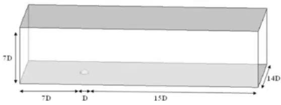
A systematic validation for the CFD code was performed. The process to study the validation considered simulation of the pressure distribution contours. Computational data were compared with experimental data as given by Cheng and Fu [4] for

L-type dome i.e. dome with diameter 120 cm (Fig.1).

Figure 1: Computational domain around dome

  2

d im e n s io n a l _{1 2}

p r e s s u r e P

n o n  _{ }

 

 

 

 

 

(8)

d i m e n s i o n a l n o n

A x i a l v e l o c i t y V

V i n l e t

_ _

 

 

(9)

The entire turbulent k-ε models were considered for the validation i.e. standard k-ε model, realizable k-ε model and RNG k-ε model. The geometry has been modeled and meshed in the preprocessor GAMBIT and then exported to FLUENT for the simulation and result predictions. Fig. 2 shows the computational domain along with meshing of dome structure.

The boundary condition at the inlet was

given as ‘velocity inlet’ and at the outlet it was given

as ‘pressure outlet’. Remaining front, back, top,

bottom and the surface of the hemispherical

structure were defined with ‘no slip wall’ boundary

condition. Pressure based solver was being used with upwind scheme for the discretization of the model equations. Finite volume based technique was used to convert the governing equations to algebraic equations that can be solved numerically. Implicit formulation and standard wall function was used. Grid independency test was being carried out before proceeding further.

Figure 2: Meshing of computational domain along with hemispherical dome

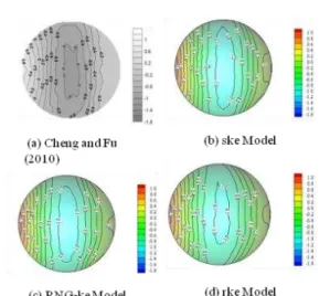
Experimental results of wind tunnel test for boundary layer flow (Cheng and Fu [4]) with Reynolds Number Re =5.2×105 and Re =7.5×105 were plotted in the non-dimensional form. Figs. 3 and 4 show the pressure contour and mean pressure distribution on centre meridian with experimental results. The comparisons of both results illustrates that the realizable k-ε model shows good agreement with the experimental data. Therefore, after validation, the realizable k-ε model was used to study some of the aerodynamic characteristics over the dome structure.

Figure 3: Comparison of mean pressure distribution contours around L-type dome (Cheng and Fu [4]) at

Re=5.2×105 in boundary layer flow

Figure 4: Comparison of mean pressure distribution on centre meridian around L-type dome

(Cheng and Fu [4]) at Re=7.5×105

IV.

RESULTS

AND

DISCUSSION

In the present study, simulation of flow past hemispherical dome is carried out through CFD code Fluent. The turbulent based models i.e. standard k-ε model, realizable k-ε model and RNG k-ε model are assessed for their ability to validate the experimental pressure distribution contours. Extensive studies of aerodynamic characteristics over hemispherical structure have been done with the help of normalized pressure, velocity and turbulent intensity contours at various vertical planes.

Figure 5: Contour plot for Cp around

hemispherical dome

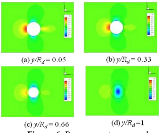
To examine the pressure distribution more specifically iso-contours of normalized pressure (Fig. 6) around hemispherical dome at different vertical plane (y/Rd=0.05, 0.33, 0.66 and 1) has been

plotted. It is observed that the pressure at the stagnation point is maximum at location y/Rd = 0.05

and as we move in vertically upward direction it decreases and shows a lesser value at that point.

Figure 6: Pressure contour around hemispherical dome at different vertical plane

In other hand, a low pressure zone is observed at the back side of the dome which also changes in the same fashion as seen for the stagnation point. Therefore, the dome exerts a pressure difference in the direction of the flow which develops a drag force on the dome surface. It is also observed that the drag force is high at location y/Rd =

0.05 (ground level) as compare to other location. Therefore, it can be concluded that the hemispherical structures experiences less force on the upper portion, which is very important for the stability of any inflatable structure. The value of drag coefficient (Cd) has been calculated by using frontal

area of the structure and it is found out to be 0.32.

Figure 7: Axial velocity contour around hemispherical dome at different vertical plane

Fig. 7 shows iso-contour for normalized velocity around hemispherical dome at different vertical planes. Fig. 7(a) depicts the region of negative velocity in the downstream of the hemispherical structure. The width of this region is seen to be maximum at this location. A reverse flow region is also observed in the downstream of the dome at this particular location which gradually disappear with the height of the dome (Figs. 7b to 7d). The high velocity zone can be observed on the both sides of the dome which is gradually increasing with the height of the dome. This increase in velocity is due to decreasing area of circular dome. However, the identification of this area will help in placing the object around and nearby the dome structure.

Figure 8: Turbulent intensity contour around hemispherical dome at different vertical plane

Fig. 8 shows the turbulent intensity plots on the same four vertical location of the dome. The highest turbulent intensity is seen in the wake of the hemispherical dome at the location y/Rd = 0.05 and

these values decreases abruptly with the height of the dome. This is due to the higher instability of flow after the separation take place. The maximum value of the turbulent intensity can also be seen near the separation point of the flow that decreases in the downstream of the flow. However, the turbulent intensity becomes approximately equal to free stream turbulence at 2.5D downstream of the flow.

hemispherical dome, the study has been extended for the parametric studies. For this, different cases of turbulent intensity have been chosen on the basis of different wind condition in India. The result has been plotted in the form of pressure contours (Coefficient of pressure, Cp) at vertical location for

y/Rd = 0.05 (Fig.9) and graph between drag force

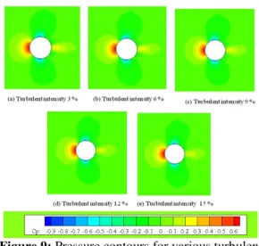
and turbulent intensity (Fig.10). The pressure contour plot as shown in Fig. 9 shows that the increase in turbulent intensity does not affect the pressure on the frontal portion of the dome but it intensively affect the pressure on the downstream of the dome structure. A negative pressure coefficient can be observed on the both side of the dome, which is due to formation of separation and flow reversal after the separation of boundary layer.

Figure 9: Pressure contours for various turbulent intensity

Fig.10 demonstrates the variation of drag force due to increase in turbulent intensity. The result shows that the increase in turbulent intensity at the inlet increases the drag on the dome. It is observed that the coefficient of drag increase approximately 9% for a medium turbulent wind condition while it increases up to 14% for a highly turbulent wind condition (i.e. 15%).

Figure 10: Effect of turbulent intensity on drag

Therefore, it is recommended for a high wind conditions that the area for the installation of hemispherical dome should have low turbulent intensity region. Usually, it is assumed that the increase in turbulent intensity decreases the drag on the curved surfaces due to shifting of the separation point in the downstream. Nevertheless, this occurrence is valid until the Reynolds number less than 105. A similar observation can be seen in the experimental result of Cheng and Fu [4] which demonstrated that the drag force first decrease until

Re≈105

and then increase gradually till Re= 106.

V.

CONCLUSION

Study for aerodynamic characteristics over the hemispherical surface was carried out. The validation pressure contour shows that the realizable k-ε model is very much close with the experimental result. It is thus demonstrated, the adequate capability of the k-ε model for performance prediction of these type of structures. The value of drag coefficient (Cd) on the hemispherical structure

is found less than other conventional structures. In the present study, the drag coefficient (Cd) has been

calculated by using frontal area of the structure and it is found out to be 0.32. Further, the value of drag coefficient (Cd) has been found intensively affected

by inlet turbulent intensity. The results with different wind conditions shows that the increase in turbulent intensity in the flow field highly influences the drag force and it increase approximately 14% for a highly turbulent wind condition (i.e. 15%).

REFERENCES

[1]. N. Toy, W.D. Moss and E. Savour, Wind Tunnel Studies On a Dome in Turbulent Boundary Layers, Journal of Wind Engineering and Industrial Aerodynamics, 1983, 201-212.

[2]. T. J. Taylor, Wind pressures on a hemispherical dome, Journal of Wind Engineering and Industrial Aerodynamics, 1991, 199-213

[3]. Fluent 6.3, User Guide Fluent Inc., Lebanon, NH 03766, 2006, USA

[4]. C.M. Cheng, and C.L. Fu, Characteristic of Wind loads on a hemispherical dome in smooth flow and turbulent boundary layer flow, Journal of Wind Engineering and Industrial Aerodynamics, 2010, 328-344 [5]. J.O. Hinze, Turbulence (McGraw-Hill

Publishing Co., New York, 1975)