Lavinia Hollanda
Essays on Economic Regulation
ESSAYS ON ECONOMIC REGULATION
Tese submetida à Escola de Pós-Graduação em Economia da Fundação Getulio Vargas como requisito para a obtenção do título de Doutor em Economia
Área de concentração: Economia
Professor Orientador: Humberto Moreira
Tese submetida à Escola de Pós-Graduação em Economia da Fundação Getulio Vargas como requisito para a obtenção do título de Doutor em Economia
Área de concentração: Economia
Aprovado em 09/07/2012 pela comissão examinadora
Humberto Moreira (Orientador, EPGE - FGV)
Carlos Eugênio da Costa (EPGE - FGV)
Cecília Machado Berriel (EPGE - FGV)
Vinícius do Nascimento Carrasco (PUC - RIO)
Agradecimentos . . . viii
Chapter 1 - Regulation Under Stock Maket Information Disclosure . . . 1
Chapter 2 - A Microdata Approach to Household Electricity Demand in Brazil . . . 33
Agradecimentos
Agradeço,
Ao meu orientador Humberto Moreira, pela paciência e por me mostrar que o único caminho possível era o da dedicação.
Aos membros da Banca Examinadora, pelo tempo dispensado na leitura deste trabalho e pelos comentários e críticas.
Aos meus co-autores Rafael Mourão, Victor Pina Dias, Joísa Saraiva e Pedro Hemsley, por tornarem este trabalho melhor e mais divertido.
Ao corpo docente da EPGE, por me ensinar uma nova maneira de pensar.
Ao professor Carlos Eugênio, pelas excelentes aulas de micro I, que foram fundamentais para que eu aprendesse todo o resto.
Aos funcionários da EPGE, por todo o apoio.
A Rebecca Barros, amiga que se tornou indispensável ao longo desses anos, pelas risadas e longas conversas.
A todos os meus colegas da EPGE, pelas conversas e debates no hall dos elevadores, pelas muitas dúvidas tiradas e pelo companheirismo.
Aos meus amigos de fora da EPGE, por toda uma vida de amizade.
Aos meus pais e irmãs, por estarem sempre por perto e pelo apoio ao longo de toda a minha vida.
Ao meu pai José de Hollanda Caldas Filho, que me ensinou desde cedo o prazer de aprender.
A minha sogra Carolina, por dedicar tanto carinho a minha filha durante as minhas ausências.
A minha filha Amelia, por ser uma criança feliz e segura que, mesmo sem saber, me ajudou a concluir esse trabalho com tranquilidade.
Chapter 1
Regulation Under Stock Maket
Information Disclosure
Lavinia Hollanda and Rafael Mourão.
It is known that stock prices of public listed regulated companies react to price revi-sions by the regulator, and that the information conveyed by this price reaction might be used by the regulator on the contract design. This paper builds on Laffont and Tirole’s (1986) regulation model with observable costs to better understand the effects the inclu-sion of the stock market can have on the regulator-regulated firm relationship. Our nu-merical simulations show that the inclusion of the market induce more powerful incentive schemes, with higher cost-reducing efforts, smaller informational rent by the firms and higher overall social welfare. In particular, we find that when the regulator is committed, the presence of short-term investors can make the first-best contract feasible, and that in the non-commitment case the market affects the firm’s strategy by making it reveal more information about its cost than it normally would.
JEL Classification:L50, L51, G30
1.1
Introduction
The relationship between a regulator and a regulated firm has been the subject of vari-ous studies, and the new economics of regulation1, which has applied the principal-agent methodology to modeling the contractual relationship between regulators and regulated firms, has provided many important insights into how this interaction takes place. How-ever, many other factors external to the regulation per se, such as political aspects or the firm’s governance structure, can impose significant constraints2 and influence this inter-action. This article is concerned with one specific factor which we believe can alter the interaction between regulator and regulated firm: public listing of the regulated firm.
In practice, examples can be found where the regulator has somehow reconsidered or revised an existent regulatory policy after observing the price performance of the regu-lated companies’ stock. One of the most striking cases of such revision was the case of the UK electricity regulator in the first periodic tariff revision in 1994, as mentioned in Faure-Grimaud 2001. Also in the electricity sector, the recent methodology changes im-plemented by the Brazilian regulator, Aneel, for the third periodic tariff cycle (RTP)3have generated widespread complaints from the regulated companies, and raised some ques-tions about the stability of the rules, and the regulator’s commitment. Without judging its merit, we believe that these recent changes can be at least partially attributed to the distri-bution companies’ performance in the market. During the second RTP cycle, even though the market’s opinion on the tariff adjustment announced usually ranged from neutral to slightly negative4, the performance of most of the companies in the quarter following the adjustment was positive5, which could indicate that those adjustments were not too strict. On the other hand, when the changes in method for the third RTP cycle were an-nounced, reports showed the market’s concern on the companies’ ability to maintain their profitability, and some analysts recommend a cautious approach to the sector for the sub-sequent years. It seems quite clear, thus, that the regulator’s decision affects the stock price of companies, mainly because the regulator’s decision has direct impact on the companies’
1See Laffont, 1994. 2See Laffont, 1994.
3For more details on the changes for the third periodic tariff cycle please see “Resolução Normativa
no 457/2011, de 08/11/2011” and "PRORET - Procedimentos de Regulação Tarifária", on Aneel’s website
(www.aneel.gov.br).
4Reference: companies’ and analysts’ reports.
profitability.
In this context, the question that arises whether factors external to regulation, such as the public listing of a company in the market, can have an impact on the regulator-regulated-firm relationship. In other words, does listing of a regulated company in any way change the relationship between the regulator and the company?
This paper examines the impact of public listing on this relationship. The basic idea underlying our work is that publicly traded companies are required to provide informa-tion to the market on their financial statements on a regular basis, and this informainforma-tion is observable to other parties – particularly, it is observable to the regulator. Since market prices usually react to this information, traded firms have a desire to demonstrate that they are efficiently managed, which usually means showing low costs and high profitability to their shareholders.
On the other hand, the theory of regulation affirms that the relationship between the regulator and the regulated firm is built based on the assumption that the regulator is at an informational disadvantage as to the firm’s operational structure and cost figures. As such, the firm is reluctant to reveal too much information about its cost structure, fearing that this information will be used by the regulator in the future to impose harsher efficiency goals. In a static environment, or when the regulator can commit to a long-term contract, the firm reveals itself in exchange for an informational rent. However, if the regulator is not committed, there is no guarantee that he will not expropriate the firm once the firm reveals itself as being efficient.
In practice, it is quite easy to find examples where stock prices of listed regulated com-panies reacted to regulators’ announcements of price revisions, but it is not as common to see situations where the regulator reacts to stock prices. Nevertheless, the notion that market prices convey information about the firm’s performance is undisputed. The basic purpose of the model is thus to understand whether the presence of the market can affect the firm’s behavior towards the regulator and the contracts offered by the regulators to the firm.
1.1.1 Related Literature
builds on a regulation model where the regulator defines a price cap depending on his knowledge about the firm’s cost parameter – which, in turn, depends on the regulator’s costly monitoring technology. There is also a model for the market, to explain how stock prices can be informative of the firm’s value. Particularly, in the Faure-Grimaud model the information collection by the regulator and the stock price information are substitutes. Thus, there will be less monitoring by the regulator when the firm is publicly listed.
The basic concept behind the model in Faure-Grimaud (2001) is the regulator’s inability to commit to long-term regulation. Due to this lack of commitment, the presence of the market can make it easier for the regulator to obtain information about the firm (in his article, through a costly monitoring technology), and expropriate its profit.
The present article builds on the same motivation. However, differently from Faure-Grimaud (2001), we endogenize the disclosure of information by the firm. We do that through the introduction of a signaling game, where the manager of the firm can actively choose the signal he will divulge to the market – and, consequently, to the regulator. Also, in our case the regulator does not have access to any particular costly monitoring technol-ogy, thus the only information available to the regulator is the (public) signal sent by the firm.
To model the firm’s signaling game, we build from the model developed by Miller and Rock (1985), in which the authors analyze the effects of announcement of dividends on the market’s perception of the firm’s profitability under asymmetric information. In their article, Miller and Rock build a signaling model that explains why dividend increases should be regarded as positive news for stock prices, from the idea that firms can signal their future profitability by paying dividends6.
One important aspect of their model (which we also incorporate in our model) is the assumption that there are two types of investors in the firm. On one side there are the “in-siders”, who are represented by the companies’ managers and are better informed about the firm’s real intrinsic value. On the other side, there are “outsiders”, who are essentially short-term investors in the market and do not observe the firm’s real value and trade their stock based on the firm’s perceived value, right after the dividend announcement7. Thus, there is a fraction of the shares which are owned by outsiders, while the remainder of the
6Basically, dividends are viewed as costly signals of future earnings, and are paid at the expense of forgone
corporate investments.
7For this reason, in Miller and Rock (1985) outside investors are viewed as short-term investors, while
shares belong to the insiders – and the objective function of the firm incorporates their re-spective weights, proportionally to the value of their holdings. In our model, described in section 3, we borrow from Miller and Rock the idea of having two types of investors (long-and short-term) in the firm.
Di Tella and Kanczuc (2003) also use that idea of incorporating market information to regulation. They propose a simple linear mechanism to punish regulated firms who outperform the market during rate reviews periods, as a way to prevent cost padding. However, their focus is mainly on the benefits of using stock prices to reduce the informa-tion problem, and not on the commitment problem. From this aspect, we view our work as more related to Faure-Grimaud (2001), since we also consider the lack of commitment on the part of the regulator as a crucial underlying assumption of our model.
Other articles acknowledge the ability of market prices to convey information on firms. Particularly, Bond, Goldstein and Prescott (2010) do so in the context of analyzing the ef-fect of government policies that aim to help firms in trouble on the informational content of market prices. Lehar, Seppi and Strobl (2007) perform a similar analysis in the context of banking regulation, but focusing on the theoretical foundations of market-based bank regulation. Despite being based on the central idea of analyzing the interaction between market prices and (some type of) government intervention in firms, both articles are de-veloped in a different context from ours, and are not directly related to our work.
The idea of our model is to understand how the existence of a third agent (the market), which can also observe the firm’s cost signal, could potentially alter the relationship be-tween the regulator and the regulated firm. Specifically, we want to model the trade-off the firm faces when sending the cost signal, from the premise that the firm wants to appear efficient to the market, and inefficient to the regulator. In a situation where the regulator is not committed and the regulated firm is publicly traded, we analyze the role of the market in the relationship between the firm and the regulator. Our main contribution is that the level of information disclosure of the firm is endogenous in our model, where the firm can actively choose whether to reveal itself or not. We use a signaling game similar to that in Miller and Rock (1985), where the signal in our case is the level of costs that the firm makes known publicly.
and the market, mainly due to the existence of a costly monitoring technology used by the regulator. Here, the regulator benefits from the presence of the market, particularly by reducing the amount of informational rent left to the efficient firm, and thus the regulator and the market can be seen as being complementary to each other.
This article is organized as follows: in a preliminary analysis, we present a basic reg-ulation model for both the full information and asymmetric information cases, which is the basis for our model. Next, we introduce a new agent to this set up: the short-term investors in the stock market. In section 3, we develop our model and discuss the (bench-mark) commitment case, and the non-commitment case. Section 4 presents a numerical simulation of the model, while section 5 concludes.
1.2
Preliminary analysis
In this section, we introduce our problem by presenting a simple, static regulation model. After introducing the main elements of the model, we solve the static, full information case and then the static problem under imperfect information. This model is presented in Laffont and Tirole (1986). We also introduce another important addition of our model, the market.
1.2.1 Full information
Suppose a regulator who wishes to provide some type of public service with valueS >0
to consumers. Consider a model where a firm capable of providing such service has cost function:
C=θ−e,
whereθis an exogenous parameter of efficiency of the firm andeis an (endogenous) effort
that the manager can exert to reduce costs. Exerting effort has a cost, given byψ(e)8.
The regulator makes net monetary transfers t to the firm and costs are fully reim-bursed9. We assume that tranfers to the firm can only be funded by taxes and, due to distortionary taxation, there is a costλ > 0 incurred by the planner for collecting
pub-lic funds, such that each unit of tranfers to the firm costs(1 +λ)to the regulator. Thus, 8This function satisfies the usual properties: ψ′
(e) > 0andψ′′
(e) > 0fore > 0, withψ(0) = 0and
lim
e→θψ(e) = + ∞.
consumer’s welfare is
S−(1 +λ)(t+C)
and the firm’s utility level is given by
U =t−ψ(e),
which implies thatt=U +ψ(e).
In the full information setting, the regulator observes both the cost and the parameter
θ. Her problem is then to choose a pair(t, e)to maximize the welfare function
WF I = S−(1 +λ)(t+θ−e) +U (1.1)
= S−(1 +λ)(θ−e+ψ(e))−λU,
subject to
U ≥0. (1.2)
The individual rationality constraint (2) says that the utility level of the firm’s manager must be nonnegative for the firm to participate in the contract. In other words, the util-ity derived by the manager from the contract should be higher than its opportunutil-ity cost (which we normalize to zero). The optimal solution for the problem is then
t = ψ(e)
e = e∗
, whereψ′
(e∗
) = 1.
1.2.2 Asymmetric information
Under imperfect information, the regulator can only observe the level of net transfertand the firm’s costC- but not its decomposition between the firm’s inherent costθand efforte.
We assume the parameterθ∈ {θL, θH},withθH > θL,is known only to the firm’s manager,
and the other agents in the economy know only its prior distributionP r[θ=θL] =ν1.
The contract offered to the firm by the regulator is a menu(t(θ), C(θ)), of transfers and
observed costs. According to the Revelation Principle, the regulator can restrict herself to direct, truthful mechanisms t(θ), C(θ) .F ornotationalsimplicity, letusmaketL ≡ t(θL),
CL≡C(θL),and so forth.
The rent of a firm of typeθwhen it selects the contract designed for its type is
and, also for notational simplicity,UL=tL−ψ(θL−CL)andUH =tH −ψ(θH −CH).
It is the incentive compatibility constraint that guarantees that each firm chooses the contract designed for its own type in the menu of contracts. For the static problem under imperfect information, those constraints are:
tL−ψ(θL−CL)≥tH−ψ(θL−CH) (1.3)
tH −ψ(θH −CH)≥tL−ψ(θH−CL). (1.4)
Similarly, individual rationality for this case amounts to
UL≥0 (1.5)
UH ≥0. (1.6)
The regulator will solve the objective function
WAI =Eθ[S−(1 +λ) [C(θ) +ψ(θ−C(θ))]−λU(θ)], (1.7)
subject to the incentive and individual rationality constraints for both types, shown above in equations (3)-(6). The solution to this problem is10
ψ′
(eL) = 1 (oreL=e
∗
) (1.8)
ψ′(eH) = 1−
λ
(1 +λ)
ν
(1−v)Φ
′
(eH), (1.9)
whereΦ(eH)≡ψ(eH)−ψ(eH−∆θ), with∆θ=θH−θL,is the informational rent obtained
by the efficient firm.
These results illustrate the basic trade-off faced by the regulator, namely, that in order to induce more effort from the inefficient firm, the regulator has to leave more informational rent to the efficient one.
1.2.3 Market signalling
In addition to the two agents described above, the firm and the regulator, we now intro-duce a third agent: the short-term investors in the stock market (henceforth, the market). As in Miller and Rock (1985), we suppose that there exists an asymmetry of information
between the firm’s long-term investors (such as managers and directors of the firm), who are considered insiders and have private information about its costs, and the short-term investors, who have no private information and are considered outsiders to the firm.
This asymmetry of information leads to differences in the perceived value of the firm for the different types of investors. The insiders are interested in maximizing the firm’s profits, defined as a function of the true inherent costθand the chosen contractθ˜11as
U(θ,θ˜) =t(˜θ)−ψ(θ−C(˜θ)).
On the other hand, the outsiders are interested in maximizing the market value of the firm. The market value function Um(˜θ) is a function that assigns a market value for the
firm based on the chosen contract . This function is known to the firm and is taken into account in its cost choice. A regular assumption about the behavior of the stock market is that, if all the participants are equal and have the same information, no expected profit can be made from trading. Thus, assuming that long-term investors plan on keeping their stocks, in equilibrium the market value of the firm is defined as a function of the chosen contract by the zero expected profit condition:
Um(˜θ) =Eθ(U(θ,θ˜)|C =C(˜θ)),
which states that the market value of the firm is given by what short-term investors believe is the firm’s profit, given the contract the firm chooses. If the market believes each firm selects its own contract, as in the basic model depicted in the past sections, the firm’s market value would be its real profit. However, differences may arise if the market believes the firms randomize.
The presence of short-term investors generates a potential conflit of interests between stockholders, since the best decision for increasing profit may not be the one that max-imizes the market value, and vice-versa. For example, even if the two contracts yield the same profit for the inefficient firm, choosing the other type’s contract can maximize market value since the market may believe that the firm is efficient with positive probabil-ity. Therefore, the firm’s objective function should take into account this conflict, so that neither type of investors have incentives to bribe the managers to depart from the firm’s optimal strategy.
11In the remainder of this paper, we will useθas both the private information parameter of the firm, as, for
Following Miller and Rock (1985), we use as objetive function a simple "social welfare function", in which the manager attach weights to each group’s utility based on its propor-tion of holdings. Thus, if the fracpropor-tion of long-term investors isk, the manager’s objective
function can be written as
U(θ,θ˜) = kU(θ,θ˜) + (1−k)Um(˜θ)
= kU(θ,θ˜) + (1−k)Eθ(U(θ,θ˜)|C =C(˜θ))
For notational ease, for the rest of this paper, U(θ, θ) andU(θ, θ) will be denoted by
U(θ)andU(θ).
1.3
The model
Our model builds on the basic, static model presented on the past section by introducing a second period, as in Laffont and Tirole (1988), and the third agent, represented by the market. In this second period the regulator may or may not make changes to the con-tract based on the information obtained in the first period, depending on whether she is commited or not. In the case of non-commitment, the firm has to take into account that the information it reveals - in addiction to affecting its market value - may also lead the regulator to make changes in the contract. For simplicity, we will only address the second period in the non-commitment case, treating the commitment case as a one-period case.
The problem can be described as a signalling game. In period one the regulator initially offers a set of contracts to the firm, which has private information about its own type
θ ∈ {θL, θH}.Both the market and the regulator have prior beliefs thatP r[θ=θL] = ν1.
By choosing a contract, the firm discloses some information for both the regulator and the market and, upon observing the realized cost, they update their beliefs aboutθ.
The posterior beliefν2is the probability given by the agents for the firm to be efficient,
given the contract it chooses. The posterior assumes valuesνH orνL when, respectively,
the high or the low cost contracts are chosen in period one. Denoting by xL and xH,
respectively, the probabilities that the efficient and the inefficient firms choose the low cost contract, according to Bayes’ rule we have
νL= xLν
1
xLν1+xH(1−ν1)
and
νH = (1−xL)ν
1
(1−xL)ν1+ (1−xH)(1−ν1)
.
Acting accordingly to this update, the short-term investors of the firm will trade their stocks based on its expected value, so the firm’s welfare is realized at
U(θ,θ˜) =kU(θ,θ˜) + (1−k)Um(˜θ)
where
Um(θH) =νHU(θL, θH) + (1−νH)U(θH)
Um(θL) =νLU(θL) + (1−νL)U(θH, θL).
In the second period, there are only long-term investors at the firm. The regulator, who also has a long term relationship with the firm, will revise the contract based on her posterior beliefs. The regulator problem will therefore be equivalent to the asymmetric information problem of the previous section.
It is also assumed that both the regulator and the firm’s manager discount the second-period welfare with factorδ >0. The regulator welfare is then
W =S−(1 +λ)(t1+C1) +U(θ,θ˜) +δ[S−(1 +λ)(t2+C2) +U(θ,θ˜)]
Finally, let us assume:
A1.The "true" (or "fundamental") value of the firmU(θ)cannot be negative.
Formally, an equilibrium in this setting can be defined as follows:
Definition 1 Let the regulator’s strategy be an incentive schemeC1 → t1(C1)in period 1, and
C2 → t2(C2;t1(.), C1) in period 2. Assume that the reservation utility of the firm is zero, and
thus the firm can choose not to participate in the relationship at any time in the game. The firm’s strategy is a choice of participationχτ and efforteτ in each period,and we letχτ = 1if the firm decides to accept the incentive scheme in periodτ, andχτ = 0otherwise.Thus, for each period the firm’s strategy is:
{χ1(θ, t1(.)), e1(θ, t1(.))}
and
The strategies and beliefs above define a Perfect Bayesian Equilibrium (PBE) of the game be-tween the regulator, the firm and the market if, and only if:
(I){e2(.), χ2(.)}is optimal for the firm givent2(.);
(II)t2(.)is optimal to the regulator given his posterior beliefs;
(III) {e1(.), χ1(.)} is optimal for the firm given t1(.) and that both the regulator’s incentive
scheme for period 2 and the market value of the firm depends onC1;
(IV)t1is optimal for the regulator given sequential strategies;
(V) the market value is defined givenC1by the zero expected profit condition
Um(˜θ) =Eθ(U(θ,θ˜)|C1 =C(˜θ)),
and;
(VI) both the market and the regulator posterior beliefs are equal and derived from the priorν1,
from (III),t1(.)andC1 using Bayes’ rule.
As mentioned earlier, the objective of our model is to understand how the interac-tion between the firm and the market could affect the regulator’s contract design. On the regulator-firm side, the model builds on the dynamic regulation model presented in Laf-font and Tirole (1988). On the firm-market side, we introduce elements from the model presented in Miller and Rock (1985), as a way to endogenize the presence of the market in the firm’s decision. In the following subsections, we will initially present the case of commitment, where the regulator can commit in the future to regulatory contracts offered in the first period. This will be our benchmark case. Next, we will analyze the case of non-commitment.
1.3.1 The commitment case
We define our commitment benchmark case as the case whereδ = 0,interpreted as having only one period. The problem faced by the regulator is very similar to the one presented in Section 2, and can be written as
max
t(.),C(.)Eθ,θ˜[S−(1 +λ)(t(˜θ) +C(˜θ)) +U(θ,
˜
subject to
U(θL)≥0 (1.10)
U(θH)≥0 (1.11)
U(θL)≥ U(θL, θH) (1.12)
U(θH)≥ U(θH, θL). (1.13)
Assuming Assumption 1 is valid at the optimum, it is easy to show (Appendix I) that, whenever constraint ICL (equation (12)) is satisfied andCH ≥ CL, then constraint ICH
(equation (13)) is also satisfied. Particularly, constraint ICH is slack only ifCH > CL.Thus,
we have thatxH = 0.
Proposition 2 Under commitment, the equilibrium is separating.
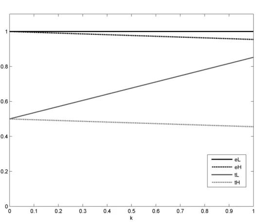
Our numerical results for the commitment case show that, for all sets of parameters used, the equilibrium is separating (xL = 1), and, as in the model exposed in Section
2.2, effort of the efficient type is always the first best (or, eL = e∗), as expected. Also,
as we increase the presence of short-term investors, both the effort and transfers made to the inefficient type increase, while the transfer made to the efficient type decreases. One possible explanation for this effect is that an increase in the proportion of short-term investors in our model means that manager is more concerned about those investors, and so the direct profit gain from deviating would have a smaller effect on her welfare.
Additionally, not only the effort and transfer for the inefficient firm increases, but it also converges to the first best askapproaches zero. Particularly, in the extreme case wherek
equals zero, there would only be short-term market investors, and the manager would care only about the expected value of the firm. Thus, there would be no direct gains for the manager to deviate other than the difference in the market value. Anticipating this, the regulator will offer contracts where the firm’s profit is zero, for either type, and the first-best would be feasible.
Corollary 3 Under commitment, the presence of the market may induce first best contracts.
Figure 1.1: Commitment case - numerical results (x-axis:k; y-axis:tL, tH, eL, eH for
ψ(e) = 12e2. Value of parameters:
1.3.2 Non-commitment case
In the non-commitment case, the parties cannot commit to a long-term contract. Instead, the relationship between the firm and the regulator is run by a series of short-term con-tracts, and the regulator might use information acquired from this relationship to expro-priate the firm. In other words, whenever the firm reveals its type, the (non-committed) regulator will review its initial contract and leave the firm with no future rent. This is the basis of the dynamic regulation model presented in Laffont and Tirole (1988), which is a special case of our model, when there are only long-term investors holding the firm’s shares (k= 1).
However, as explained in the beginning of this section, our model has a third partic-ipant to this relationship: the market. Since the firm’s manager is concerned with both short-term investors (who hold a fraction(1−k) of the firm’s shares) and long-term in-vestors, there is a conflict between the information the firm wants to reveal to the market and to the regulator. Ideally, the efficient firm would want to show to the market that it is operationally efficient (since the market trades basd on the firm’s expected value), while not revealing its type fully to the regulator (since it could be expropriated later on). The main purpose is to analyze how the presence of the market affects the relationship between the regulator and the regulated firm in both cases.
For the second period,WF I(ν)andWAI(ν)are the optimal expected one-period
wel-fare under full information and under incomplete information, respectively, for priorv.
For the two-type case we are investigating, we assume there are two contracts being of-fered by the regulator, (tL, CL) and (tH, CH). Thus, the regulator maximizes the following
expected welfare:
WN C = S−(1 +λ)νxL(tL+CL) +U(θL, θL)
−(1 +λ)ν(1−xL) (tH+CH) +U(θL, θH)
−(1 +λ)(1−ν)xH(tL+CL) +U(θH, θL)
−(1 +λ)(1−ν)(1−xH) (tH +CH) +U(θH, θH)
subject to
U(θL)≥0 (1.14)
U(θH)≥0 (1.15)
U(θL) +δΦ(eH(νL))≥ U(θL, θH) +δΦ(eH(νH)) (1.16)
U(θH)≥ U(θH, θL), (1.17)
whereΦ(eH(ν2))is the informational rent left for the efficient firm at the second period to
induce revelation.
One perverse effect generated by the lack of commitment from the regulator is clear from the intertemporal incentive compatibility for typeθL(equation (16)).Since, by
reveal-ing itself, the efficient firm will be expropriated at the second period (eH(νL)is decreasing
toward zero), there are more incentives for the efficient firm to choose the inefficient con-tract. It is also important to note that the rent for the inefficient type at the second period will always be zero, even if the contracts are separating and it pretends to be efficient. This happens because, without commitment, the firm can leave the relationship after the first period, in a take-the-money-and-run strategy.
The possibility of this kind of action by the inneficient firm is the cause of greater part of the complexity of the problem, and induces some types of equilibrium where both ICs are binding, when regularly only the incentive compatibility for typeθLis binding. This
happens because, to generate incentives for the efficient firm to exert effort, compensating the second period expropriation, the principal has to increase transfers made to the effi-cient firm, making the effieffi-cient contract more attractive for the innefieffi-cient firm, who can take the transfers and leave the relationship before having to exert first-best efforts at the second period.
1.4
Example and comparative statics
To analyze the behavior of the model described above, we do some comparative statics in the special case where the disutility of effort has a quadratic form:ψ(e) = 12[max(0, e)]2.12
We will use this special case to study numerically the effect of the presence of the market in our model. All numerical simulations where run with the software Matlab R2012a, as detailed on Appendix III.
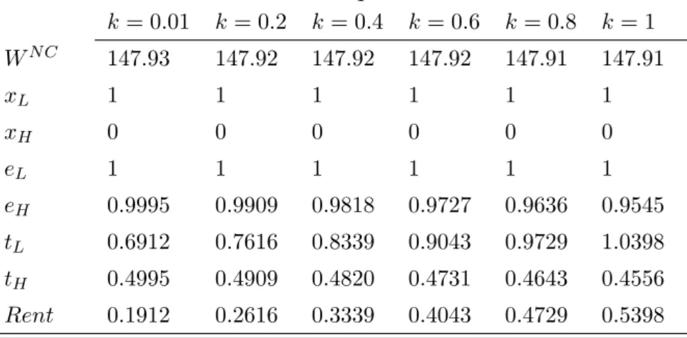
To proceed with our analysis, we chose a set of parameters to define a basis non-commitment case and analyzed the equilibrium behavior for different levels of market participation (i.e., askvaries from 0 to 1). Table 1.1 shows the numerical results.
Table 1.1: Results for benchmark equilibrium - selected values of k
k= 0.01 k= 0.2 k= 0.4 k= 0.6 k= 0.8 k= 1
WN C 147.93 147.92 147.92 147.92 147.91 147.91
xL 1 1 1 1 1 1
xH 0 0 0 0 0 0
eL 1 1 1 1 1 1
eH 0.9995 0.9909 0.9818 0.9727 0.9636 0.9545
tL 0.6912 0.7616 0.8339 0.9043 0.9729 1.0398
tH 0.4995 0.4909 0.4820 0.4731 0.4643 0.4556
Rent 0.1912 0.2616 0.3339 0.4043 0.4729 0.5398
Value of parameters:S= 100, θL= 1.5, θH = 2, ν = 0.5, λ= 0.1, δ= 0.5
In Table 1.1, it is possible to see that the presence of the market leads to more powerful incentives, inducing more effort from the inefficient firm. Moreover, the rent of the efficient firm decreases and welfare increases as the share of short-term market investors increases (kdecreases). For this set of parameters, the best equilibrium is always a separating one,
regardless of the amount of market investors in the firm.
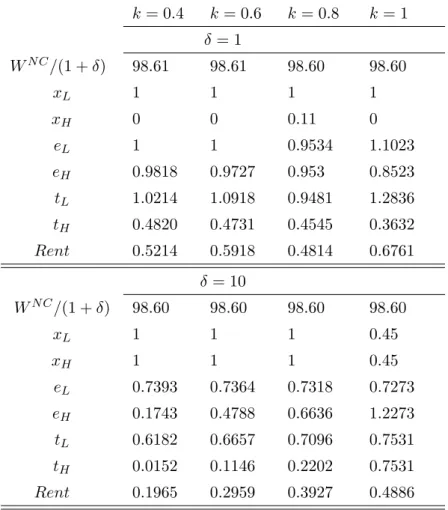
From this benchmark equilibrium, we vary some of the parameters to understand their effects on the equilibrium. As a first exercise, we evaluate our model when we vary the
12There is a similar numerical exercise in Laffont and Tirole (1988), so our results could, to some extent, be
Table 1.2: Comparative statics for intertemporal discount rate
k= 0.4 k= 0.6 k= 0.8 k= 1
δ= 1
WN C/(1 +δ) 98.61 98.61 98.60 98.60
xL 1 1 1 1
xH 0 0 0.11 0
eL 1 1 0.9534 1.1023
eH 0.9818 0.9727 0.953 0.8523
tL 1.0214 1.0918 0.9481 1.2836
tH 0.4820 0.4731 0.4545 0.3632
Rent 0.5214 0.5918 0.4814 0.6761
δ= 10
WN C/(1 +δ) 98.60 98.60 98.60 98.60
xL 1 1 1 0.45
xH 1 1 1 0.45
eL 0.7393 0.7364 0.7318 0.7273
eH 0.1743 0.4788 0.6636 1.2273
tL 0.6182 0.6657 0.7096 0.7531
tH 0.0152 0.1146 0.2202 0.7531
Rent 0.1965 0.2959 0.3927 0.4886
Value of parameters:S= 100, θL= 1.5, θH = 2, ν = 0.5, λ= 0.1
intertemporal discount rateδ.As a general result, for small, positive δ13 the best
equilib-rium is still a separating equilibequilib-rium, but asδincreases, we find that the equilibrium starts to show some degree of pooling or a semiseparation(xL < 1). However, when the
par-ticipation of the market increases, the separating equilibrium continues to dominate, even for larger discount factors(δ= 10, shown in Table 1.2). Table 1.2 shows some results for
different values of discount factors and proportions of long-term investors (k).
Based on these results, the presence of the market induces more separation - for a fixed value ofδ, separating equilibrium dominates askdecreases. Also, welfare increases and
the informational rent of the efficient type decreases when the proportion of shares in the market increases. The effort of the inefficient type also increases in this case, showing again
that the presence of the market leads to more powerful contracts.
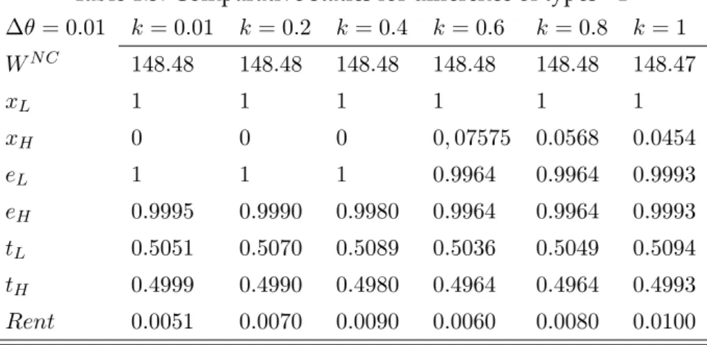
Also, we analyze the effect of varying the difference between the technological pa-rameters for the types,∆θ,in the equilibrium. As a general rule, the equilibrium tends more towards a pooling as∆θdecreases. However, we see some interesting results as we
vary the amount of market participation: for a given∆θ, the increased participation of
short-term market investors leads to more separation. Putting this differently, separating equilibrium was dominant fork <0.5in all cases analyzed. This means that the presence
of the market might induce separation, even when∆θis too small (we analyzed the case for∆θ = 0.01) - which can viewed as a positive effect of the market. However, as∆θ
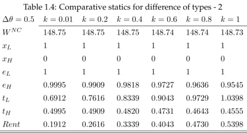
in-creases, we see that the presence of the market becomes less important, since separation is always optimal for∆θlarge enough. Tables 1.3 and 1.4 show those results.
Table 1.3: Comparative statics for difference of types - 1
∆θ= 0.01 k= 0.01 k= 0.2 k= 0.4 k= 0.6 k= 0.8 k= 1
WN C 148.48 148.48 148.48 148.48 148.48 148.47
xL 1 1 1 1 1 1
xH 0 0 0 0,07575 0.0568 0.0454
eL 1 1 1 0.9964 0.9964 0.9993
eH 0.9995 0.9990 0.9980 0.9964 0.9964 0.9993
tL 0.5051 0.5070 0.5089 0.5036 0.5049 0.5094
tH 0.4999 0.4990 0.4980 0.4964 0.4964 0.4993
Rent 0.0051 0.0070 0.0090 0.0060 0.0080 0.0100
Value of parameters:S= 100, θL= 1, θH = 1.01, ν = 0.5, λ= 0.1, δ= 0.5
We can summarize our results in the following propositions:
Proposition 4 In a separating equilibrium, the presence of the market increases welfare, reduces informational rent and leads to more powerful incentives.
Proposition 5 Whenever there is a separating equilibrium for a givenk∗
, there will be a separating equilibrium for allk≤k∗
.
Table 1.4: Comparative statics for difference of types - 2
∆θ= 0.5 k= 0.01 k= 0.2 k= 0.4 k= 0.6 k= 0.8 k= 1
WN C 148.75 148.75 148.75 148.74 148.74 148.73
xL 1 1 1 1 1 1
xH 0 0 0 0 0 0
eL 1 1 1 1 1 1
eH 0.9995 0.9909 0.9818 0.9727 0.9636 0.9545
tL 0.6912 0.7616 0.8339 0.9043 0.9729 1.0398
tH 0.4995 0.4909 0.4820 0.4731 0.4643 0.4555
Rent 0.1912 0.2616 0.3339 0.4043 0.4730 0.5398
Value of parameters:S = 100, θL= 1, θH = 1.5, ν = 0.5, λ= 0.1, δ= 10
to the firm. In this sense, differently from Faure-Grimaud (2001), we view the presence of the market as complementary to regulation, as it helps the regulator to achieve a more efficient outcome, but without being its substitute.
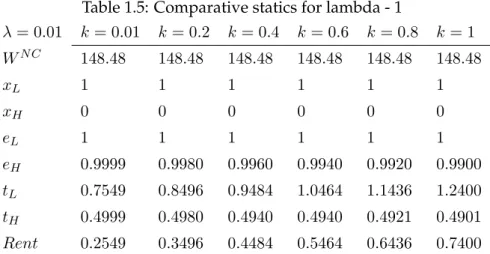
Lastly, by changing the values of the prior probabilityνand of the cost of public fundsλ
we have separating equilibria for all cases, for all values ofk.Thus, the results for changes in those parameters are as expected from the theory: asν increases, the amount of
infor-mational rent left to the efficient firm to reveal itself decreases, since the regulator has a stronger prior belief that the firm’s type is efficient; as we vary the cost of public funds
λ, both expected rent and welfare decrease whenλdecreases, and the effort level for the
inefficient type is also reduced. Clearly, as public funds become more expensive, it is more costly for the regulator to make transfers, and thus the level of efforts is lower.
Regarding the effect of the market for varying the prior beliefν or the cost of public funds (λ), informational rent decreases and welfare increases askapproaches zero - which
corroborates our previous results regarding the effect of the presence of market, namely that the presence of the market seems to have a positive effect on welfare. Appendix III shows some simulation results for different values ofνandλ.
1.5
Conclusion
the relationship between the regulator and the regulated firm. For this purpose, we used a signaling model, where the level of information disclosure of the firm was endogenous, and the firm could choose whether or not to reveal itself. Our basic premise was that the firm wants to appear efficient to the market, and inefficient to the regulator.
Appendix I
The commitment case for our model (section 1.3.1):Consider
U(θj) =kUj + (1−k)E[U(θ)|C=Cj]
where
Uj =tj −ψ(θj −Cj),
forj=L, H. We then have
UL = kUL+ (1−k)νLUL+ (1−νL)U(θH, θL)
UH = kUH+ (1−k)
νHU(θL, θH) + (1−νH)UH
.
We also know that the deviation payoff of both types (i.e.U(θ,θb),whereθbis the announce-ment made by typeθ) in terms of the truthful announcement and the rent can be written
as: when typeθLannouncesθH, we have
U(θL, θH) = k[tH −ψ(eH−∆θ)] + (1−k)E[U(·)|C=CH]
= k[tH −ψ(eH−∆θ)]−k[tH−ψ(eH)]
+k[tH −ψ(eH)] + (1−k)E[U(·)|C=CH]
| {z }
=U(θH)
U(θL, θH) = U(θH) +kΦ(eH).
Similarly, when typeθH announcesθL, we have
U(θH, θL) = k[tL−ψ(θH−cL)] + (1−k)E[U(·)|C =CL]
= k[tL−ψ(θH−cL)]−k[tL−ψ(θL−CL)]
+k[tL−ψ(θL−cL)] + (1−k)E[U(·)|C =CL]
| {z }
=U(θL)
U(θH, θL) = U(θL)−kΦ(eL+ ∆θ).
Thus, we can write ICLand ICH,respectively, as
UL ≥ UH +kΦ(eH)
UH ≥ UL−kΦ(eL+ ∆θ).
Also, it is trivial to show that constraints ICLand IRH together (equations (1.12) and (1.11))
constraints ICLand ICH together, we have
kΦ(eH) ≤ ICL
UL− UH ≤
ICH
kΦ(eL+ ∆θ),
which implies thatCL≤CH. Substituting the expression forULintoUH, we have
0≥k[Φ(eH)−Φ(eL+ ∆θ)],
which is true, since we already showed thatCL≤CH.Particularly, ICH is slack whenever
CL < CH - and, in this case, xH = 0. Notice also that ICL is binding, otherwise the
regulator would be leaving too much rent to the effcient firm.
Appendix II
In this Appendix, we make some calculations similar to those done in Laffont and Tirole (1988). We calculate the expressions for equilibria type I, II and III for our model. Differ-ently from Laffont and Tirole (1988), our model has a third agent, the short-term investors in the market, as described in Section 1.3.
For these calculations, we restrict ourselves to the set of direct and truth-telling con-tracts. Given the menu of contracts offered by the regulator, denote the deviation payoff of firm with typeθwhich “announces”θˆbyU(θ,θˆ). Hence,
U(θi, θj) =kU(θi, θj) + (1−k)Eθ[U(θ)|C=Cj],
whereU(θi, θj) = tj−ψ(θi−Cj), fori, j∈ {L, H}. Let us also denote the firm’s
informa-tional rent of typeθi by
Ui=U(θi) =U(θi, θi), i∈ {L, H}.
Equilibrium Type I:For this equilibrium, the inefficient type playsCH with probability 1
(remember that only the ICLconstraint is binding). Thus, we have
xH = Pr [C=CL|θ=θH] = 0⇒vL= Pr(θ=θL|C=CL) = 1.
This means that, whenever the market observesCL being played in this equilibrium, it
knows with certainty that this is the efficient type. We thus have that
Also, when the market observes a signalCH, we have that
Eθ[U(θ)|C =CH] =νHU(θL, θH) + (1−νH)U(θH).
From the binding incentive compatibility constraint (equation (1.16)), we have that
U(θL) =
k+ (1−k)νHΦ(eH) +δ[Φ(e(νH))−Φ(e(νL))] (1.18)
and
tL=ψ(eL) +U(θL). (1.19)
From Assumption 1 we have thatU(θH) = 0, thus
tH =ψ(eH) (1.20)
andU(θH) = (1−k)νHU(θL, θH), or
U(θH) = (1−k)νHΦ(eH). (1.21)
We are now ready to calculate the expected welfare for a type I equilibrium:
WI =S−(1 +λ)ν1xL(tL+CL) +ν1(1−xL) (tH +CH) + (1−ν1) (tH +CH) +ν1xLU(θL) +ν1(1−xL)U(θL, θH) + (1−ν1)U(θH)
+δν1xLWF I(1) +ν1(1−xL) + (1−ν1)WAI(νH)
Substituting equations (1.18), (1.19), (1.20) and (1.21) and rearranging we have
WI =S−(1 +λ)ν1xL[ψ(eL) +CL]−(1 +λ)ν1(1−xL) [ψ(eH −∆θ) +CH]
−(1 +λ)(1−ν1) [ψ(eH) +CH]
+ν1(1−xL) [k−(1 +λ)]−λν1xLk Φ(eH) +(1−k)νHν1(1−xL) + (1−ν1)−λν1xL
Φ(eH)
+δν1xLWF I(1) +
ν1(1−xL) + (1−ν1)
WAI(νH)
−λν1xLδ[Φ(e(νH))−Φ(e(νL))].
This is the welfare function for a type I equilibrium.
Equilibrium Type II:In a type II equilibrium, it is the efficient type that chooses his own contract (CL) with probability 1. In this case we have
Here we have only the incentive compatibility constraint for the inefficient type (equation (17)) binding and, when the signal observed iscH,the market knows with certainty that it
is the innefficient type playing:
Eθ[U(θ)|CH] =U(θH) =U(θH).
When the signalCLis observed, we have
Eθ[U(θ)|C=CL] =νLU(θL) + (1−νL)U(θH, θL).
From the individual rationality constraint for the inefficient type binding we know that
U(θH) =U(θH) = 0 (1.22)
and
tH =ψ(eH). (1.23)
Also, from the incentive compatibility of the inefficient type also binding, we have
U(θH, θL) = 0
which implies that
U(θL) =kΦ(eL+ ∆θ). (1.24)
Finally, we know that
U(θL) =k+ (1−k)νLU(θL) + (1−k)(1−νL)U(θH, θL),
and we find
U(θL) =
k+ (1−k)(1−νL)
[k+ (1−k)(1 +νH −νL)]Φ(eL+ ∆θ)
and
tL=ψ(eL) +
k+ (1−k)(1−νL)
[k+ (1−k)(1 +νH −νL)]Φ(eL+ ∆θ). (1.25)
We now can express the welfare function for a type II equilibrium
WII =S−(1 +λ)ν1(tL+CL) + (1−ν1)xH(tL+CL)
−(1 +λ)(1−ν1)(1−xH) (tH +CH)
+ν1U(θL) + (1−ν1)xHU(θH, θL) + (1−ν1)(1−xH)U(θH)
and, after substituting equations (1.22), (1.23), (1.24) and (1.25),we find
WII =S−(1 +λ)ν1[ψ(eL) +CL]−(1 +λ)(1−ν1)xH[ψ(eL+ ∆θ) +CL]
−(1 +λ)(1−ν1)(1−xH) [ψ(eH) +CH] +(1 +λ)(1−ν1)xH+ν1kΦ(eL+ ∆θ)
−(1 +λ)ν1+ (1−ν1)xH
k+ (1−k)(1−νL)
[k+ (1−k)(1 +νH−νL)]Φ(eL+ ∆θ) +δν1+ (1−ν1)xH WAI(νL)
+(1−ν1)(1−xH)
WF I(0) .
This is the expression for the welfare in a type II equilibrium.
Equilibrium type III: In a type III equilibrium, the incentive compatibility for both types are binding, so the market cannot identify the player for either signal. Thus
Eθ[U(θ)|C=CL] = νLU(θL) + (1−νL)U(θH, θL)
Eθ[U(θ)|C=CH] = νHU(θL, θH) + (1−νH)U(θH),
where the posteriors are
νH = ν
1(1−x
L) (1−ν1)(1−x
H) +ν1(1−xL)
νL = ν
1x
L
xH(1−ν1) +ν1xL
.
From Assumption 1 and optimality, we know thatU(θH) = 0,which implies that
U(θL) = [k+ (1−k)νL]U(θL) + (1−k)(1−νL)U(θH, θL)
and
U(θH) = (1−k)νHΦ(eH). (1.26)
From the incentive compatibility of the effcient type binding, and from equation the ex-pression forU(θL, θH)in appendix I, we have
U(θL) =U(θH) +kΦ(eH) +δΦ(e νH)−Φ(e νL) (1.27)
which implies, by substituting equations (1.26) and (1.27):
[k+ (1−k)νL]U(θL) + (1−k)(1−νL)U(θH, θL)
Also, from incentive compatibility of the ineffcient type binding, and from the expression forU(θH, θL), we have
U(θH) =U(θH, θL) =U(θL)−kΦ(eL+ ∆θ).
Then, using equations (1.26) and (1.27), and knowing thatU(θL, θH) = Φ(eH),we find
[k+ (1−k)νL]U(θL) + (1−k)(1−νL)U(θH, θL) = (1−k)νHΦ(eH) +kΦ(eL+ ∆θ).
We can now solve the following system:
[k+ (1−k)νL]U(θL) + (1−k)(1−νL)U(θH, θL)
= k+ (1−k)νHΦ(eH) +δΦ(e νH)−Φ(e νL)
[k+ (1−k)νL]U(θL) + (1−k)(1−νL)U(θH, θL)
= (1−k)νHΦ(eH) +kΦ(eL+ ∆θ).
This will happen if, and only if
δΦ(e νH)−Φ(e νL)=k[Φ(eL+ ∆θ)−Φ(eH)].
To solve fortL,we use the first equation in the system above and find
tL = [k+ (1−k)νL]ψ(eL) + (1−k)(1−νL)ψ(eL+ ∆θ) (1.28) +(1−k)νH +kΦ(eH) +δΦ(e νH)−Φ(e νL). (1.29)
Finally, we substitutetLintoU(θL) =tL−ψ(eL)andU(θH, θL) =tL−ψ(eL+ ∆θ),
rear-range, and find
U(θL) = [(1−k)(1−νL)]Φ(eL+ ∆θ) +(1−k)νH +kΦ(eH) +δΦ(e νH)−Φ(e νL)
(1.30) and
U(θH, θL) =(1−k)νH +kΦ(eH)−[(1−k)νL+k]Φ(eL+∆θ)+δΦ(e νH)−Φ(e νL).
objective function for a type III equilibrium. The regulator will solve
WIII = S−(1 +λ)ν1xL[ψ(eL) +cL]−(1 +λ)(1−ν1)xH[ψ(eL+ ∆θ) +cL]
−(1 +λ)ν1(1−xL) [ψ(eH−∆θ) +cH]
−(1 +λ)(1−ν1)(1−xH) [ψ(eH) +cH]
−λν1xLkΦ(eL+ ∆θ)
+ν1(1−xL) [k−(1 +λ)] Φ(eH)
+ (1−k) (1 +λ)(1−ν1)xHΦ(eL+ ∆θ)
+(1−k)νH1−(1 +λ)(1−ν1)xH +ν1xL Φ(eH)
−(1−k)(1−νL)(1 +λ)(1−ν1)xH+ν1xLΦ(eL+ ∆θ)
+δν1xL+ (1−ν1)xHWAI(νL) +ν1(1−xL) + (1−ν1)(1−xH)WAI(νH)
s.t. k[Φ(eL+ ∆θ)−Φ(eH)] =δΦ(e νH)−Φ(e νL)
Appendix III
As mentioned in Section 1.3.2, all numerical simulations were implemented with the use of the software Matlab R2011b. In this appendix we outline the procedure used to find the equilibrium of the dynamic problem and the results for different sets of parameters.
For each case, including the commitment (δ = 0), the problem was solved for all three
types of equilibrium, as defined in the Appendix II. For each type of equilibrium and randomization strategies, it is possible to find the optimal contract for the regulator - so the welfare function can be rewritten in terms of the exogenous variables(S, θL, θH, λ, ν and
δ)and randomization profiles. Those welfare functions were then numerically optimized
forxLandxH using Matlab’s in-built optimizing functionfminconwith several uniformly
Table 1.5: Comparative statics for lambda - 1
λ= 0.01 k= 0.01 k= 0.2 k= 0.4 k= 0.6 k= 0.8 k= 1
WN C 148.48 148.48 148.48 148.48 148.48 148.48
xL 1 1 1 1 1 1
xH 0 0 0 0 0 0
eL 1 1 1 1 1 1
eH 0.9999 0.9980 0.9960 0.9940 0.9920 0.9900
tL 0.7549 0.8496 0.9484 1.0464 1.1436 1.2400
tH 0.4999 0.4980 0.4940 0.4940 0.4921 0.4901
Rent 0.2549 0.3496 0.4484 0.5464 0.6436 0.7400
Value of parameters:S= 100, θL= 1, θH = 2, ν = 0.5, λ= 0.01, δ= 0.5
Table 1.6: Comparative statics for lambda - 2
λ= 1 k= 0.01 k= 0.2 k= 0.4 k= 0.6 k= 0.8 k= 1
WN C 146.87 146.83 146.79 146.77 146.75 146.75
xL 1 1 1 1 1 1
xH 0 0 0 0 0 0
eL 1 1 1 1 1 1
eH 0.995 0.9 0.8 0.7 0.6 0.5
tL 0.7549 0.83 0.87 0.87 0.83 0.75
tH 0.4950 0.405 0.32 0.245 0.18 0.125
Rent 0.2549 0.33 0.37 0.37 0.33 0.25
Table 1.7: Comparative statics forν1- 1
v= 0.1 k= 0.01 k= 0.2 k= 0.4 k= 0.6 k= 0.8 k= 1
WN C 147.68 147.68 147.68 147.68 147.68 147.68
xL 1 1 1 1 1 1
xH 0 0 0 0 0 0
eL 1 1 1 1 1 1
eH 0.9998 0.9979 0.9959 0.9939 0.9919 0.9898
tL 0.7549 0.8495 0.9484 1.0463 1.1435 1.2398
tH 0.4999 0.4979 0.4959 0.4939 0.4919 0.4899
Rent 0.2549 0.3495 0.4483 0.5463 0.6435 0.7398
Value of parameters:S = 100, θL= 1, θH = 2, ν = 0.1, λ= 0.1, δ= 0.5
Table 1.8: Comparative statics forν1- 2
v= 0.7 k= 0.01 k= 0.2 k= 0.4 k= 0.6 k= 0.8 k= 1
WN C 146.87 146.83 146.79 146.77 146.75 146.75
xL 1 1 1 1 1 1
xH 0 0 0 0 0 0
eL 1 1 1 1 1 1
eH 0.9978 0.9575 0.9151 0.8727 0.8303 0.7878
tL 0.7549 0.8415 0.9160 0.9736 1.0142 1.0378
tH 0.4978 0.4584 0.4187 0.3808 0.3447 0.3103
Rent 0.2549 0.3415 0.4160 0.4736 0.5142 0.5378
dation, 2004.
[2] Bond, Philip, Itay Goldstein and Edward S. Prescott, "Market-based Corrective Ac-tions",The Review of Financial Studies,23 (2), 781-820, 2009.
[3] Camacho, Fernando T. and Flavio Menezes, "Price Regulation and the Cost of Capi-tal",Working Paper, University of Queensland, 2010.
[4] Di Tella, Rafael and Fabio Kanczuc, "Stock-price Based Regulation", Department of Economics Working Paper 300, University of Brasilia, 2003.
[5] Faure-Grimaud, Antoine, "Using Stock Price Information to Regulate Firms",The Re-view of Economic Studies, 69 (10), 169-190, 2002.
[6] Kyle, Albert S., "Continuous Auctions and Insider Trading",Econometrica,53, 1315-35,
1985.
[7] Laffont, Jean-Jacques and Jean Tirole,A Theory of Incentives in Procurement and Regula-tion,Cambridge and London: MIT Press, 1993.
[8] Laffont, Jean-Jacques and Jean Tirole, "The Dynamics of Incentive Contracts", Econo-metrica, 56, 1153-75, 1988.
[9] Laffont, Jean-Jacques and Jean Tirole, "Using Cost Observation to Regulate Firms", The Journal of Political Economy, 94 (3), 614-41, 1986.
[11] Miller, Merton and Kevin Rock, "Dividend policy under asymmetric information",
Chapter 2
A Microdata Approach to Household
Electricity Demand in Brazil
Lavinia Hollanda, Victor Pina Dias and Joisa Dutra Saraiva
Over the recent years, many players in the Brazilian electricity sector have demon-strated rising concerns related to security of supply. Instead of the usual capacity expan-sion solution, a different approach to the energy shortage issue would be to adopt demand side management (DSM) mechanisms. These mechanisms could lead to a more rational electricity consumption in Brazil. Our study focus on pricing-related issues as a way to shed some light on how consumers respond to price changes. This is an important starting point to the implementation of DSM mechanism. The purpose of the study is to estimate price elasticities of demand using microdata, by investigating the behavior of the house-hold consumer in the different regions of the country, with the aim at understanding the drivers for household electricity consumption. The results observed in the context of the energy efficiency discussion may inform alternative regulatory policies that could induce electricity consumers to reduce their consumption in response to price changes, eventually contributing to broader energy efficiency goals.
JEL Classification:D12, L94.
2.1
Introduction
The goal of assuring security of supply and reasonable prices for all the stakeholders in the electricity industry pressures both policy makers and regulators. In this context, the adoption of demand response (DR) mechanisms could create significant welfare gains.
There is compelling evidence that consumers change their behavior pattern once ex-posed to time-varying prices. Hence dynamic pricing mechanisms could result in im-provement of efficiency in relation to the most commonly observed flat rates – which tend to result in overconsumption at peak times and underconsumption during off-peak peri-ods.
The response observed in terms of reduced consumption as a result of the implemen-tation of price and quantity rationing mechanisms can be further enhanced with the in-troduction of smart grid1 (SG) technologies. Additionally, to fully benefit from DR, con-sumers must be endowed with advanced metering infrastructure (AMI). The current dis-cussion on the adoption of SG technologies in Brazil takes this potential into account.
In this context, considering that the required investments in SG technologies are high, it is of paramount importance to evaluate the potential of demand response that can be achieved. A government’s decision to stimulate adoption of the required infrastructure depends on the assessment of the net benefits that can be achieved. The high costs involved must be compared with the expected benefits in order to induce the investments at a pace that is consistent with consumers’ payment capacity, and also their disposition towards the new infrastructure that has to be put in place. Thus it is very important to understand to what extent consumers are willing and/or are able to decrease demand in response to higher prices. This question has already motivated many efforts to estimate demand price elasticity, and the answers to it can help in shaping AMI investment decisions.
The purpose of this study is to estimate price elasticity of electricity demand for res-idential consumers in Brazil using microdata from the Brazilian Consumer Expenditure Survey for the years 2002-2003. To our knowledge, this is the first work that has been done to estimate electricity demand price elasticity in Brazil from data disaggregated at the household level.
1The term “Smart grid” generally refers to technologies involving computer-based remote control and
Estimating price elasticity of electricity demand, however, can pose a lot of challenges, particularly if residential consumers face flat tariffs – as is the case in Brazil. The data set used is this paper does not allow us to observe a single household at two different times; but we do have access to data on similar households in different periods. We use three different specifications in our estimates: (i) a pseudo-panel approach; (ii) a first difference approach; and (iii) a two-stage approach.
This paper is organized as follows: in section 2.2, we frame our work in the context of the demand response debate. We discuss the relevance of DR programs in electricity mar-kets, and the importance of understanding consumers’ responses to price changes when participating in such initiatives. Section 2.3 offers a brief review of the empirical literature on estimation of price elasticity of demand in the electricity sector, mainly focusing on the residential segment. The data set and the pseudo-panel specifications with estimation re-sults are described in section 2.4, while section 2.5 contains estimation rere-sults for the first difference estimator. In section 2.6 we report the results for the two-stage, derived-demand specification. Finally, Section 2.7 gives our conclusions.
2.2
The relevance of demand response in electricity markets
Over recent years, many players in the Brazilian electricity sector – and particularly the government and regulators – have shown increasing concern on the security of supply. Historically, the approach to overcome this problem has been to expand installed capacity. However, increasing environmental concerns, the high levels of investment required to build new power plants, and even the difficulty of finding new sources of clean, renewable and economically viable sources of energy add complexity to the subject.
A different – and far more contemporary and appealing – approach to ensuring secu-rity of supply would be to implement demand response and energy efficiency measures to rationalize energy consumption in Brazil. Globally, such environmental and supply con-cerns, coupled with the need to make the electricity sector more competitive and reliable, have strengthened the arguments in favor of energy conservation measures.
topics such as the integration of distributed generation into the grid, and implementation of price mechanisms to induce energy conservation and reduce the future impact on the environment.
In many European countries and in the US, utilities and regulators are already imple-menting energy policies targeting energy efficiency. These include: (i) advocating for new appliance and building standards to induce energy savings; (ii) investing in smart grid technologies and financing and/or subsidizing consumers’ investments in advanced me-tering infrastructure (AMI); (iii) encouraging distributed generation, especially when us-ing renewable sources of energy; (iv) creatus-ing mechanisms to decouple utilities’ revenues from the volume of kilowatt-hours (kWh) sold to consumers, to stimulate utilities to ad-here to such initiatives, and so forth. Also, distinct demand side management mechanisms have been successfully adopted in several countries, particularly in the US.
In Brazil, government efforts2 toward a more effective energy efficient policy are still very timid; and mechanisms to induce consumer response through prices are mostly non-existent in the residential sector, despite the explicit commitment to security of supply.
All the above-mentioned initiatives are important for promoting energy conservation. However, to enhance the effectiveness of such measures, and to reach allocative efficiency, it is key to implement rate mechanisms that better reflect the marginal cost of providing electricity to consumers at any given time. An efficient rate design should be the starting point of any energy rationalization policy put in place by government authorities and reg-ulators. So it is important to evaluate the extent to which consumers are able to change their behavior in response to time-varying prices.
The majority of consumers in Brazil are charged flat rates for the electricity they con-sume. A tariff structure that charges different prices depending on the period of consump-tion is only available to large (industrial) consumers. More recently, the Brazilian electricity regulator (Aneel) has proposed a new tariff structure that allows low voltage consumers (small businesses and residential consumers) to opt in for time varying rates within the day. This new rate design is to come in effect after 2014.3
Basic economic theory posits that efficient prices should reflect marginal costs. In the
2These initiatives include the “Programa Nacional de Conservação de Energia Elétrica” (Procel) and the
requirement that distribution companies invest 1% of their net operational revenues in R&D and energy effi-ciency programs.
3For more details on the new approved tariff structure, to be applied from 2014 on, please see “Resolução
electricity sector, this would imply that for a given stock of capital and appliances in the economy, allocative efficiency could be improved by replacing current flat retail prices with rates that better reflect the underlying marginal cost of producing an additional kilowatt-hour under those circumstances and at that time - and that this should result in a more efficient distribution of resources4.
Adoption of dynamic pricing mechanisms of course requires an evaluation of the ex-pected benefits net of the exex-pected costs of implementation. In the high voltage segment (i.e. industrial consumers), it is well accepted that the deployment of time-varying rates induces a more rational use of electricity. Industrial consumers show considerable price-elasticity of demand5and many European countries as well as North American states have adopted time-varying prices for this segment for quite some time.
The cost-benefit ratio has not been so clearly established for low-voltage clients (e.g. small businesses and residential consumers), particularly due to the high costs usually as-sociated with the deployment of the metering infrastructure necessary to reap the benefits of a “smarter” rate design6. On the other hand, technological improvements have reduced the costs associated with AMI, and prices for metering and communication technologies have been falling in recent years, indicating the possibility of a larger potential client base being suitable to participate in demand response programs. Also, since AMI can further enhance the potential customer response to dynamic pricing (and vice-versa),– this inter-relation has to be investigated in any analysis of the cost-benefit of installing AMI.
One factor possibly explaining resistance to change in flat electricity rates for residen-tial consumers is the potenresiden-tially high political cost associated with the implementation of time-varying rates. Regulators and government authorities are concerned with the re-action of consumers (essentially, voters) to volatility in electricity prices. In this situation, rather than being allowed to vary, retail prices remain flat all year round, even during peri-ods of drought, when it is often necessary to dispatch high-cost power plants to guarantee supply. Consumers end up paying this cost in the future, since the aggregate increases in costs are passed through to them in subsequent tariff reviews. They are just not given the opportunity to react when costs are high.
4See King, King and Rosenzweig, 2007.
5Industrial customers might show different figures for price-elasticity due to strong differences in their
production processes. Nevertheless, some of the studies analyzed in Bohi and Zimmerman (1984) show price elasticities higher than unity (in absolute value) for industrial consumers in the US.
6Nevertheless, to obtain an adequate level of customer response, it is not required to have every customer
Time-differentiated rates are already in place in some other important sectors in Brazil such as telecoms, internet and cable TV, where consumers can choose different tariff de-signs according to their profile. The experience in some of these sectors indicates the possi-bility of consumers having the option to subscribe to time-differentiated rate regimes after being presented with the costs and benefits of opting-in to them.
Finally, implementing DR and energy efficiency measures will require the support of the many stakeholders involved in the electricity sector. One of the most important group of stakeholders is the distribution companies. In the current regulatory framework in Brazil they do not have effective incentives to promote energy efficiency. The costs they incur to acquire the energy they need are mostly passed through to consumers. Hence they have no incentive to reduce the costs associated with buying energy.
Also, under the current pricing mechanisms, any initiatives that aim to reduce kilowatt-hours sold will reduce companies’ revenues. With rates in Brazil, as in many other coun-tries, set on a simple per-unit basis, it is quite difficult to get distribution companies to voluntarily support policies aimed at reducing electricity consumption. To overcome this resistance, there is a need for debate on new regulations that would mitigate or eliminate the link between volume and revenue.
All these points indicate that proposing and implementing a new rate design that al-lows customers to respond to varying prices will not be simple. On the contrary, it will require a thorough analysis of consumer behavior, deployment of appropriate metering and communication infrastructure, and an investigation of the underlying costs and bene-fits.
The starting point of any careful analysis is investigation of consumers’ behavior. The effectiveness and feasibility of any benefits depend on the real willingness of consumers to respond to price changes by modifying their demand for electricity. Since different types of consumers may respond in a different way to price changes, it is essential to understand the behavior of each category of consumer – industrial, commercial, residential. Almost all of the numerous studies so far made on this question have concluded that consumers do respond to price changes7.
It is also necessary to evaluate to what extent demand response is efficient. In other words, a demand response program should be implemented only if there are net benefits. This reasoning needs to be established for each distinct group of consumers.