Echinococcus multilocularis
Infection in Foxes
Fraser I. Lewis1, Belen Otero-Abad1, Daniel Hegglin2, Peter Deplazes2, Paul R. Torgerson1*1Section of Veterinary Epidemiology, University of Zu¨rich, Zu¨rich, Switzerland,2Institute of Parasitology, University of Zu¨rich, Zu¨rich, Switzerland
Abstract
Characterizing the force of infection (FOI) is an essential part of planning cost effective control strategies for zoonotic diseases.Echinococcus multilocularisis the causative agent of alveolar echinococcosis in humans, a serious disease with a high fatality rate and an increasing global spread. Red foxes are high prevalence hosts of E. multilocularis. Through a mathematical modelling approach, using field data collected from in and around the city of Zurich, Switzerland, we find compelling evidence that the FOI is periodic with highly variable amplitude, and, while this amplitude is similar across habitat types, the mean FOI differs markedly between urban and periurban habitats suggesting a considerable risk differential. The FOI, during an annual cycle, ranges from (0.1,0.8) insults (95% CI) in urban habitat in the summer to (9.4, 9.7) (95% CI) in periurban (rural) habitat in winter. Such large temporal and spatial variations in FOI suggest that control strategies are optimal when tailored to local FOI dynamics.
Citation:Lewis FI, Otero-Abad B, Hegglin D, Deplazes P, Torgerson PR (2014) Dynamics of the Force of Infection: Insights fromEchinococcus multilocularis Infection in Foxes. PLoS Negl Trop Dis 8(3): e2731. doi:10.1371/journal.pntd.0002731
Editor:Giovanna Raso, Swiss Tropical and Public Health Institute, Switzerland
ReceivedOctober 22, 2013;AcceptedJanuary 23, 2014;PublishedMarch 20, 2014
Copyright:ß2014 Lewis et al. This is an open-access article distributed under the terms of the Creative Commons Attribution License, which permits unrestricted use, distribution, and reproduction in any medium, provided the original author and source are credited.
Funding:This work was supported by the Swiss National Science Fund, grant number CR3313 132482. The funders had no role in study design, data collection and analysis, decision to publish, or preparation of the manuscript.
Competing Interests:The authors have declared that no competing interests exist. * E-mail: [email protected]
Introduction
The force of infection (FOI) is a crucial epidemiological parameter and characterizing its dynamics is an essential part of planning cost effective control strategies for infectious diseases [1]. Mechanistically, disease intervention strategies are typically targeted at decreasing the per capita infection rate. If successful, this will then cause a decrease in observed prevalence. As such, quantification of the FOI provides a key measure of efficacy when assessing or comparing interventions [2]. The FOI can be extremely difficult to estimate directly, i.e. observationally, in wildlife populations. Even in human populations this is not without considerable challenges, and requires accurate longitudinal monitoring of the target population in order to capture all new infections which arise [3]. An alternative approach is to estimate the FOI indirectly, through access to prevalence data, in conjunction with either an explicit mathematical model describing the disease transmission processes, or else some assumed disease risk function [4,5].
Foxes are typical definitive hosts for the parasite Echinococcus multilocularis, with different rodent species being the primary intermediate host in which the alveolar hydatid cysts grow. In humans, which are aberrant hosts, this parasite causes the important emerging zoonosis alveolar echinococcosis (AE). This is a serious disease with a high fatality rate in the absence of appropriate treatment [6]. In Europe there have been increasing numbers of AE cases reported in the Baltics [7], Poland [8], Austria [9] and in Switzerland [10]: the latter associated with an increase in fox populations. The disease is also emergent in central Asia with a huge increase in the numbers of human cases in Kyrgyzstan recorded in recent years [11]. This disease also has a
considerable impact on human health in Western China, particularly on the Tibetan plateau [12]. Alveolar echinococcosis is also an emerging public health concern in North America due, at least in part, to the increasing urbanization of wild canids [13]. Red foxes (Vulpes vulpes) are high prevalence hosts ofE. multilocularis
[14], where zoonotic transmission may occur through environ-mental contamination [15] or through contaminated food [16]. In addition, dogs are susceptible definitive hosts [17] and may be very important for transmission to humans where prevalences in dogs are high, such as in China [18] or central Asia [19]. In Europe, dogs are low pravalence hosts [20], but nevertheless may pose a high risk of introducing the parasite in non endemic countries such as the UK if appropriate treatment is not given when dogs enter the country [21].
In Switzerland it has been shown that there are considerable differences in the spatial and seasonal distribution of the prevalence of E. multilocularis in definitive hosts [14,15] and intermediate hosts [23]. These studies indicated that 129 of 857
Arvicola terrestriswere infected of which 12 harboured protocolices. Ten of these animals had between 61 and 452,000 protoscolices. Seasonal patterns of infection in intermediate hosts were seen with highest prevalences seen in over-wintered animals. Thus seasonal anthelmintic treatment of foxes, with a focus on the autumn and winter months, is likely to be a more efficient strategy in reducing the parasite biomass [23]. Likewise although fox densities are highest in urban settings, they consume fewer rodents and have a greater reliance on anthropomorphic food supplies compared to rural foxes [24], which is likely to significantly affect transmission dynamics on a spatial scale. Consequently, the intensity of intervention strategies could also be tailored to exploit these spatial differences. Such differences in prevalences clearly indicate that relative differences in the FOI exist between rural and urban areas, and between winter and summer seasons.
We develop a statistically robust quantitative characterization of the FOI for E.multilocularis in foxes to address three specific research questions: i) firstly, is the FOI constant or dynamic (with age of the host), and what is its value accounting for complexities such as statistical uncertainty; ii) secondly, how much does FOI vary quantitatively with habitat type, in particular between more or less urbanized regions; iii) and thirdly how much does the FOI of infection vary quantitatively on a temporal basis between winter and summer seasons.
Methods
The key methodological aspect of this study is to identify an epidemiologically useful disease transmission model for E.multi-locularis in foxes. A model whose structure can be objectively justified, and whose parameter estimates provide tangible insight into the key infection processes. Three sources of information are available to support model development: i) prevalence data from a previously presented observational study [24]; ii) approximate estimates as to likely survival times ofE. multilocularisin foxes from experimental work [17]; and iii) existing transmission modelling frameworks for Echinococcus granulosus transmission in sheep and dogs [25]. Using [25] as a starting point, we identify a process model whose structure is an optimal fit to the prevalence data from [24], whilst making use of the parameter estimates from [17] as expert knowledge. Following [25] we utilize ordinary differential equations (ODEs) to describe the transmission dynamics, and to take advantage of prior knowledge from [17] we adopt a Bayesian paradigm [26] for all model fitting and statistical inference.
Study data
The data to which we fit our transmission models is an extension of that previously described in [14] and [24], and
includes only samples taken prior to the anthelmintic baiting intervention described in [27]. Samples were collected from in or around the city of Zurich in Switzerland. Three key variables were utilized: i) presence (absence) ofE.multilocularisinfection based on necropsy (details given in [14,24]); ii) the age of each fox, and following previous studies, and as described in [14], cubs were assumed to be born on 1st April and age determination of foxes sampled after 1st July was done via examination of teeth (details given in [14]). Along with the date of death (which is known as these animals were culled by hunters) and the weight at death, each animal’s approximate age in years and days was estimated. The final variable utilized was habitat type, where this comprised three zones reflecting differing degrees of urbanization: urban; border; and periurban. The characteristics of these are described in detail in [27]. The urban zone comprises of mostly residential dwellings with relatively few green spaces, the periurban zone is rural comprising of forests, fields, pastures, and meadows. The border zone separates urban from rural, and was defined as extending 250 meters from the edge of the urban area and into 250 meters of the periurban surroundings. The border zone includes largely residential areas, public spaces, allotments and pastures. The data used in the study is in the Supporting Information Data S1. Out of then~458foxes aged three years or less in the study data, 160 were sampled in the periurban zone, 167 in the border zone and 131 in the urban zone. The overall observed prevalence across all 458 animals was 42.1%, within the periurban, border and urban zones this was 65.6%, 38.9% and 17.6% respectively. The median age across these 458 animals was 0.80 years. In the periurban, border and urban zones the median respective ages were 0.87, 0.77 and 0.59 years.
Disease transmission model
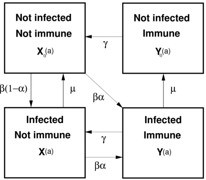
The most general form of hypothesized transmission model we consider forE. multilocularisis given in Figure 1. The structure of this model is based on initial work by [25] which has provided a basis for many subsequent disease modelling studies involving inE. granulosus and E. multilocularis, (e.g. [5,28]). Figure 1 depicts an intuitively reasonable representation of the possible disease states and flows between them based on current known biology of
E.multilocularisin foxes. The model dynamics here are over age of the host (foxes), as is typical when modelling E. multilocularis or
E.granulosus. We assume a fully susceptible population at birth, i.e. no vertical transmission and therefore X0(a)~1. This dynamic system can be described in a series of ordinary differential equations (ODEs).
State variables areX0(a),X(a), Y0(a)and Y(a), whereX0(a) represents the proportion of hosts which are not infected and not immune at agea,X(a)is the proportion of hosts which are infected and not immune at agea. VariablesY0(a)andY(a)are defined similarly but for cohorts –not infected and immune} and –infected and immune} respectively. The following system of ordinary differential equations defines the dynamics over age of this system:
dX0
da ~{bX0zmXzcY0,
dX
da~b(1{a)X0{(mzba)XzcY,
dY
da~baX0zbaX{(czm)Y, Author Summary
Human alveolar echinococcosis (AE) is caused by the fox tapeworm E. multilocularis and has a high fatality rate if untreated. The frequency of the tapeworm in foxes can be reduced through the regular distribution of anthelmintic baits and thus decrease the risk of zoonotic transmission. Here, we estimate the force of infection to foxes using a mathematical model and data from necropsied foxes. The results suggest that the frequency of anthelmintic baiting of foxes can be optimised to local variations in transmis-sion that depend upon season and type of fox habitat.
dY0
da ~mY{cY0
with initial conditions:X0(0)~1,X(0)~0,Y0(0)~0andY(0)~0. Parameterbdenotes infection pressure (force of infection - FOI), measured in insults (exposures) per year; ais the probability of immunity on exposure;cis the duration of host immunity;mis the parasite death rate. Note that to simplify the notation we have suppressed any explicit dependency of the parameters on age, e.g.
b(a)where FOI is dependent upon age, but such dependencies are considered during the model selection process making this potentially an inhomogeneous ODE system.
Model fitting and statistical analyses
The observed data comprise of randomly sampled binary observations each denoting whether a fox was infected (not infected). This gives a sampling model comprising of Bernoulli trials where the likelihood function for n observations is
Pni~1p(ai)Ii(1{p(ai))1{Ii, where ai is the age of theith fox in
the data,Ii is an indicator variable whereIi~1if theith fox is
infected and Ii~0 otherwise, and p(ai)~X(ai)zY(ai) is the
prevalence in foxes of age ai. The ODE transmission model
providesp(a)which will generally be some unknown function of the epidemiological parameters of interest, p(a)~f(a,b,c,m,a) where (Figure 1):ais the probability of immunity on exposure;b
the force of infection (measured in insults per unit time);cthe rate of loss of immunity; and m the parasite death rate. It is not necessary to know functionf explicitly, all that is required is that for any given values of a,b,c,m, along with appropriate initial conditions for state variablesX0,X,Y0,Y, an estimate forp(a)for any suitable value ofacan be computed. This is readily possible using standard numerical techniques for solving ODEs (e.g. [29]). The likelihood function (| parameter priors as we are using Bayesian inference) can therefore be evaluated, and thus the key unknown epidemiological parameters of interest such asbcan be estimated from the study data —conditional on the chosen form of ODE model.
Figure 1. Transmission model forE.multilocularisin foxes. State variables are:X0(a), X(a), Y0(a)andY(a), whereX0(a)represents the
proportion of hosts (foxes) which are not infected and not immune at agea, the other state variables are similarly defined. Parameterbdenotes the infection pressure (force of infection), measured in insults (exposures) per year;ais the probability of immunity on exposure;cis the rate of loss of host immunity;mis the parasite death rate.
Gaussian distributed prior distributions for parametersbandc
were used, where these were each implemented within a log link function. For the probability parametera, a logit link function was used, again with a Gaussian prior distribution. Highly diffuse priors were used for all parameters exceptm, where these each had a mean of zero and standard deviation ofpffiffiffiffiffiffiffiffiffiffi1000. In effect, this introduces no prior biological knowledge into the estimation of these parameters. Form, a Gaussian prior (again on a log link) was used and chosen via expert opinion based on data presented in [17]. The latter study comprised of longitudinal observation of five foxes experimentally infected with E. multilocularis. The parasite burden in 80% (three of five) animals was very low at 90 days, suggesting an 80th percentile for the death rate of approximately ƒ4per year, in addition we consider that parasites in 50% of infected animals may survive to around 120 days (death rateƒ3 per year), with 2.5% possibly surviving beyond 150 days (death rateƒ2:4per year). A Gaussian distribution on a log link with a mean of 1.2 and standard deviation of0:2, gives quantiles form(on real scale) of approximately 2.24 (2.5%), 3.32 (50.0%) and 3.93 (80%) per year, which we choose as an informative prior form. In addition we also examine a wider, but still highly informative prior, with a mean of 1.3 and standard deviation of 0.3 which has corresponding quantiles of 2.04 (2.5%), 3.67 (50.0%) and 4.72 (80%) per year. Sensitivity to prior assumptions is a crucial aspect of Bayesian inference, so we also present modelling results which use the same highly diffuse (uninformative) prior formas forband
c.
Bayesian model selection — used to identify an optimal ODE transmission model — was performed using the marginal likelihood goodness of fit metric. This is equivalent to comparing Bayes factors between two models when each has an equal a priori probability of being the preferred model. The marginal likelihood is generally more difficult to compute than other commonly used metrics, such as the Bayesian Information Criterion (BIC) or Deviance Information Criterion (DIC), but is the standard and preferred theoretical choice in Bayesian inference [26,30]. This metric allows Bayesian model selection to be interpreted as simply an extension of maximum likelihood model selection, where evidence (i.e. statistical support) for any given model is that obtained by multiplying the best fit likelihood by the ‘‘Occam factor’’, so-named as this metric has been shown to be conceptually consistent with Occam’s Razor (as explained in [30]). The marginal likelihood was computed using Laplace approximations, a standard numerical technique in statistical inference [31,32]. These were also used to estimate posterior distributions for the epidemiological parameters. All numerics were implemented in R [33] using a number of well tested internal functions borrowed from the R abn library [34]. See Supporting Information Text S1 for technical details. An approximate guide for the size of differences in marginal likelihoods which may be considered notable is given in Table 2.1 page 27 in [26]. Using the terminology from [26], a difference of0{2is suggested as weak support for the model with higher marginal likelihood, 2{6 is support,6{10is strong evidence and greater than 10 very strong evidence.
Results
We first present a brief exploration of the observed prevalence data by age. This is prudent as it may suggest refinements in the parametrization of the process models under consideration. Next we compare the goodness of fit of a range of models with different biological assumptions, for example whether the observed data support the presence of immunity, and if so, whether this is lifelong
or transient. We then quantify the key epidemiological parameters in our chosen model, in particular the FOI,b(a). Heterogeneity is then introduced into this model by allowing the force of infection to differ across one or more of the three different habitat types, where further model selection is used to identify a preferred heterogeneous model. Our results conclude with a comparison of FOI estimates across the different habitat zones.
Exploratory analyses by age
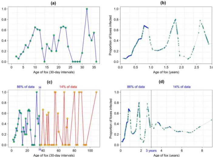
Exploratory analyses of the observed prevalence data is illustrated in Figure 2. Choosing a smoothing parameter of f = 0.072 in (lowess() in R) gives smoothed data which appear relatively consistent with the observed data in Figure 2 (a), and provides a more refined visualization of the data rather than in 30-day blocks. Figure 2 (a) and 2 (b) suggest that it may be appropriate to consider the inclusion of periodicity into one or more of the epidemiological parameters in our transmission model.This suggests that for our model to adequately capture the gross dynamic features of disease transmission we should consider both age independent FOI,b(a)~b0, and also FOI parametrized as a function of age, b(a)~g(a), with g(a) as some polynomial or periodic function. It is clear from Figure 2 (c) that there appears very little identifiable dynamic structure after 36 months, which is perhaps unsurprising given this only comprises some 14% on observations, and thus very sparse sampling at these older ages.This is consistent with life expectancy estimates for foxes which suggest that only a small proportion of foxes survive beyond 2–3 years years in the wild [35]. As foxes aged less than three years present the vast majority of zoonotic risk, combined with foxes of older ages being sampled very sparsely in the data, subsequent analyses focus on foxes less than three years of age. For completeness some modelling results are also presented consider-ing all ages. Figure 2 (d) shows the smoother applied to data of all ages.
Determining a parsimonious transmission model A range of transmission models of increasing complexity were fitted to the observed data (Table 1) with separate results shown for the two informative priors form. See Supporting Information Text S2 for results using an uninformative prior form, and Supporting Information Text S3 for the equivalent of Table 1 but for the models fitted to data from foxes of all ages. Estimates of the posterior modes for all the parameters in models presented in Table 1 can be found in Supporting Information Text S4.
Evaluation of immunity
We commenced with a model comprising no immunity (Model 1-C), i.e. only state variablesX0and X, and constant FOI. This was followed by similar models but where the FOI was parametrized as a linear (1-L), quadratic (1-Q) and periodic (1-P) function of age, with the latter using a sinusoidal forcing term as is commonly used for diseases with periodic transmission rates (e.g. measles [36]). The particular form of sinusoidal function used was
logfb(a)g~b0zb1sin 2p a{ exp(as)
1zexp(as)
. A log link
func-tion ensures that all estimates ofb(a)are positive, and also avoids the potentially complex task of having to specifying a proper (i.e. integrates to unity) joint parameter prior forb0,b1andaswhich
would otherwise be required to ensure that the posterior distribution forb(a) was positive. This parametric form of b(a) has a period of one year, with (on a log scale) b0 denoting the lifetime average (or baseline) FOI,b1 the amplitude beyond the lifetime average. The term exp(as)=(1zexp(as)) is to allow, if
Figure 2. Exploratory analyses.Panel (a) shows observed prevalence across age groups of 30-days blocks up to age 36 months (where 1 month = 30 days). Panel (b) shows smoothed prevalence using a locally weighted regression smoother (lowess() in R) applied to the 0/1 observation for all individuals aged less than 3 years. Panel (c) shows observed prevalence across age groups of 30-days blocks for all ages (maximum 108 months where again one month = 30 days). Panel (d) shows the smoother applied to data of all ages.
doi:10.1371/journal.pntd.0002731.g002
Table 1.Model goodness of fits.
Model Description Prior form Log marginal likelihood
1-C no immunity(a~0)Constant FOI:logb(a)~b0 N(1:2,0:2)N(1:3,0:3) 2305.3 (DML~28:2)
2304.3 (DML~26:2) 1-L no immunity(a~0)Linear FOI:logb(a)~b0zb1a N(1:2,0:2)N(1:3,0:3) 2309.3 (DML~36:2) 2308.9 (DML~35:4) 1-Q no immunity(a~0)Quadratic FOI:logb(a)~b0zb1azb2a2 N(1:2,0:2)N(1:3,0:3) 2308.1 (DML~33:8)
2308.3 (DML~34:2)
1-P
no immunity(a~0)Periodic FOI:logfb(a)g~b0zb1sin 2p a{ exp(as) 1zexp(as)
N(1:2,0:2)N(1:3,0:3) 2291.3 (DML~0:2) 2291.2 (DML~0:0) 2
lifelong immunity(c~0)periodic FOI:logfb(a)g~b0zb1sin 2p a{ exp(as) 1zexp(as)
N(1:2,0:2)N(1:3,0:3) 2294.3 (DML~6:2) 2294.6 (DML~6:8) 3
transient immunity(c=0)periodic FOI:logfb(a)g~b0zb1sin 2p a{ exp(as) 1zexp(as)
N(1:2,0:2)N(1:3,0:3)
2294.2 (DML~6:0) 2296.0 (DML~9:6)
All parameters other thanmhave diffuse priors as given in the text. TheDMLdenotes twice the difference between the best log marginal likelihood and each of the other models.
necessary, a time shift compared with the standard sinusoidal function. A logit link function is used here as we are only interested in time shifts in the interval [0,1]. Parametersb0,b1 andaseach
have diffuse Gaussian priors with means of zero and standard deviations ofpffiffiffiffiffiffiffiffiffiffi1000.
From Table 1 is it clear that periodic infection pressure is strongly supported over the other forms. Retaining periodic infection pressure, we next consider models with a more complex cohort structure comprising of all four state variables fX0,X,Y,Y0g, allowing for the presence of lifelong immunity (Model 2), and transient immunity (Model 3 and the ‘‘full’’ model in Figure 1). It is again apparent from Table 1 that the observed data are less supportive of these two more complex models, and hence there is little evidence in the data for the presence of immunity.
Based purely on the goodness of fit results in Table 1 our preferred model is Model 1-P. The next more complex best fitting model was Model 2. These two models cross a rather large biological divide — no immunity verses lifelong immunity. To provide additional empirical justification for choosing Model 1-P over Model 2 we briefly examine the magnitude of the parameters in the latter model using the posterior modes (which are estimated as part of the marginal likelihood computation). In Model 2, using the prior for mwith mean of 1.2, we have a logit foraof 25.3
giving an approximate probability of becoming immune per exposure of 0.005. Posterior mode estimates for the FOI in this model, b(a), gives an (approximate) average lifetime number of exposures, exp(b0), of &2 per year. Based on the observed
prevalence data, then suppose that 86% of animals have a lifetime of at most three years and the remaining 14% live for a full nine years. Then, in a population of 100 animals these parameters give a total of 768 exposures for all animals over their entire lifetime. For a~0:005 this then gives, on average, at most only four animals becoming immune during the entire lifetime of the population. This is a very fine scale population change, and it is therefore of little surprise that, statistically, the empirical data are not supportive of the presence of immunity.
Quantification of force of infection
Having arrived at a preferred transmission model we now use this to provide the first of our main results: quantification of the FOI, i.e. b(a). Of most interest here are the baseline and amplitude parametersb0andb1, specifically we wish to estimate the joint marginal posterior distribution for these two parameters and then examine the range of values for the FOI which arise when (b0,b1) are within their joint 95% posterior confidence interval (to account for sampling uncertainty). It would be possible to consider a joint density comprising of all three parameters in
b(a); b0,b1,as. It is, however, difficult to visualize such a density
(with four dimensions - three parameters plus the density estimate), and as epidemiological interest is focused on(b0,b1)we therefore marginalize out as and m giving a joint posterior density for
(b0,b1). Note that this distribution, therefore, also incorporates the statistical uncertainty inasandm(i.e. the latter are not simply fixed
at constant values).
Before computing the joint marginal density for(b0,b1)we first summarizeb0,b1,mandasthrough their marginal posterior 95%
confidence intervals (Supporting Information Text S5 provides full marginal posterior densities). Using the informative prior for m
with mean = 1.2 and sd = 0.2 gives (on the real scale)
b0~(1:32,2:79), b1~(2:27,4:55), as~(0:35,0:48) and m~(2:38,4:82), with approximate medians of b0~1:92,
b1~3:14, as~0:42; and m~3:36. The corresponding estimates
when using the informative prior for m with mean = 1.3 and
sd = 0.3 are b0~(1:34,3:34), b1~(2:29,4:55), as~(0:35,0:49)
and m~(2:30,6:14), with approximate medians of b0~2:087,
b1~3:17, as~0:42; and m~3:74. Using the diffuse prior for m
gives b0~(1:16,4:19), b1~(2:33,4:51), as~(0:38,0:54) and m~(1:69,8:25), with approximate medians of b0~2:24,
b1~3:20,as~0:50; andm~3:98.
A contour plot of the joint marginal posterior density for (b0,b1), Figure 3 panel a, clearly shows strong dependency betweenb0andb1— when one is lower the other is higher and vice-versa. This demonstrates why it is more intuitively reasonably to consider these parameters jointly. To visualize the statistical uncertainly in our estimate of FOI over age we choose two points pt1,95%~(b0,b1) and pt2,95%~(b0,b1), which lie on the contour defining the 95% region for this two-dimensional density. We then solve the ODE model for these sets of parameter estimates (the other two parameters are set to their modal values). These two ‘‘extreme’’ sets of parameters provide an approximate 95% confidence interval for the mean force of infection over age (Figure 3 panel b), and similarly the mean prevalence (Figure 3 panel c). We estimate the (mean) minimum FOI during an annual population cycle as 0.27 to 1.27 insults (with 95% confidence), and rising to a maximum of between 6.87 and 7.05 insults (with 95% confidence).
Comparison between urban and rural habitats
The summary statistics suggest that there may be a difference between the prevalence ofE.multilocularisin populations of foxes within the different habitat types. To provide a measure of statistical rigour to these observations we fit Model 1-P to these data, where now heterogeneity is introduced intob(a)to allow the force of infection to vary across each of the different zones. If the inclusion of such heterogeneity improves the model goodness of fit then that provides formal statistical evidence of a different in FOI between habitats.
We consider two versions of Model 1-P, Model 1-P0and Model 1-P01. The first allows the baseline force of infection,b0, to vary with zone and assumes the amplitudeb1is homogeneous across all zones. The second model allows bothb0 and b1 to vary within each habitat zone. For simplicity, the period shiftasand parasite
death rate m are assumed homogeneous over all three zones. Model 1-P0 has a goodness of fit of 2285.4, with Model 1-P01
having2292.6. This is strong evidence that: i) there is a difference
in baseline force of infection between different habitat zones; ii) there is no evidence of any difference in periodic amplitude between the different habitats. We use, therefore, Model 1-P0to quantify differences in FOI across habitat.
Following a similar approach as for our analyses of Model 1-P, we derive approximate confidence intervals for the force of infection using the joint marginal posterior densities forb0andb1, where this time we have three, two dimensional distributions, (bU0,b1),(bB0,b1),(bP0,b1)forUurban,Bborder andPperiurban. First we summarizebU0,bB0,bP0,b1,mandasthrough their marginal
posterior 95% confidence intervals (Supporting Information Text S6 provides full marginals posterior densities). Using the informa-tive prior form with mean = 1.2 and sd = 0.2 gives (on the real scale) bU0~(0:45,1:27), bB0~(1:20,2:94), bP0~(2:42,6:18),
b1~(1:48,3:2),as~(0:29,0:47)andm~(2:29,4:50), with
approx-imate medians of bU0~0:79, bB0~1:87, bP0~3:79, b1~2:13, as~0:38andm~3:14. It is clear that the marginal densities in the
urban and periurban habitats do not overlap at the 5% significance level. Supporting Information Text S7 provides a comparison of the modal estimates of prevalence over age in each of the three habitat types.
Finally we consider the statistical uncertainty in our FOI estimates over age within each habitat type. Figure 4 panel a is similar to Figure 3 panel a and shows the joint marginal posterior densities for(bU0,b1),(b0B,b1),(bP0,b1). As for the one-dimensional marginal estimates ofb0in each habitat, it is very clear that the FOI baseline is statistically different between the urban and periurban zones i.e. the 95% contours do not overlap. The FOI in the border zone is indistinguishable from that in either the periurban or rural zones. We repeat the same approach to estimate approximate 95% confidence intervals for the FOI within each habitat as for the homogeneous habitat model (Model 1-P), this is shown in Figure 4 panel b. These uncertainty limits are clearly rather more approximate here than for those in Model 1-P — as can be seen by the fact that the urban and periurban trajectories overlap slightly, while they are clearly very distinct at the 95% contours in Figure 4 panel a. The limits for the border habitat also cross each other. This behavior is not entirely unexpected in that we are collapsing a six dimensional posterior probability distribution (comprising of all the parameters in Model 1-P0) into effectively only two dimensions. This gives joint statistical estimates which are far more manageable, but as we see here, does makes the resulting confidence limit estimates rather approximate. We estimate with approximate 95% confidence that
the (mean) minimum FOI during an annual cycle in the urban habitat is 0.1 to 0.8 insults, rising to a maximum of between 1.6 and 2.0 insults. For the periurban habitat we have minimum and maximum force of infections of 0.7 to 3.9 insults and 9.35 to 9.7 insults respectively. Despite these minor statistical discrepancies in relation to the differing comparisons of confidence limits, the overall result is very clear: there is a large difference in FOI during annual cycles in the urban and periurban habitats.
Discussion
The FOI is a key parameter in models estimating the effectiveness and cost effectiveness of infectious disease prevention [37]. Using a simple —and empirically justified — mathematical model we have estimated the force ofE. multilocularisinfection in a fox population in Switzerland, and shown how much it quantitatively varies with season and geography, i.e. through time and across space.
There have been a number of trials aimed at reducing the prevalence of infection in foxes by distributing baits containing the anthelmintic praziquantel. Several studies, in Switzerland and in Germany, with baiting intervals of 12 times per year, resulted in a substantive decline in the numbers of foxes infected (reviewed in Figure 3. Transmission Model 1-P.Panel (a): joint marginal posterior density for(b0,b1)on log scale. The red contour is the 95% limit and the two
points marked are those used to produce approx. 95% confidence intervals in panels b and c. Panel (b): dynamics of force of infection by age, 95% CI is for the mean force of infection at agea. Panel (c): Smoothed observed prevalence and prevalence predicted by Model 1-P, 95% CI are for the mean prevalence at agea. All results use the informative prior formwith mean = 1.2 and sd = 0.2.
[22,38,39]). These studies typically resulted in a decrease in prevalence from 35% and 67% to between 1% and 6%. Provided most foxes are treated, this would be expected as the baiting interval is similar to the prepatent period ofE. multilocularisin foxes and hence it should prevent transmission. Other baiting campaigns have used lower frequencies and have had variable results. For example in Germany a baiting frequency of 5 times per year resulted in a decrease in the prevalence in foxes of 32% (95% CIs 16–52) to 4% (95% CIs 2–7). Other studies with less frequent baiting intervals have not shown such a clear reduction. Our estimates and modelling methodology for computing the
pre-intervention baseline FOI provides a rigorous framework which can be used to optimize baiting intervals, in order to trade off the need to reduce infection in foxes, and thus the potential for zoonotic transmission, and the cost of implementing such intervention programmes. Based on Swiss data we estimate that there is a high infection pressure in the winter months for non urban foxes of close to 10 infections per year (i.e. greater than 1 per month), baiting at monthly intervals would therefore be required. This conclusion is in accordance with the results of an epidemiological study on the intermediate hosts which showed most rodents become infected during the winter [23]. However, in Figure 4. Heterogeneous habitat transmission Model 1-P0.Panel (a): joint marginal posterior densities for(bU
0,b1),(bB0,b1),(bP0,b1)on log
scale. The red contour is the 95% limit and the two points marked are those used to produce approx. 95% confidence intervals in panel b. Panel (b): dynamics of force of infection by age, approx 95% CI is for the mean force of infection at agea(see main text for explanation of why these lines cross). All results use the informative prior formwith mean = 1.2 and sd = 0.2.
doi:10.1371/journal.pntd.0002731.g004
the summer when the FOI is lowered to between 0.7 to 3.9 insults per year, then decreasing the baiting frequency to once every three months would be more appropriate. In addition, baiting frequen-cy, at least in theory, could be further reduced in urban habitats where the FOI is between 0.1–0.8 and 1.6–2.0 insults per year. However in practice, this would be a challenge in Zu¨rich as the spatial separation of such zones is as little as 500 meters. A decreased cost of baiting foxes increases the cost benefit as a similar reduction in the numbers of human AE cases would be expected to be achieved as earlier suggested [15] based on epidemiological data [23,24]. Theoretical models [40,41], have also suggested seasonal transmission of E. multilocularis in Japan. However, our model is also challenged with field data, where as the conclusions of previous models are based on simulations. In addition, our model does not depend upon parameters from the intermediate host and therefore should be applicable for FOI calcualtions in any area where suitable prevalence data from foxes is available.
Our estimates of FOI are dependent on the estimate of the life expectancy of the infection in the definitive host. Experimental infections of foxes indicate that parasites can survive in foxes beyond 90 days [17], although most parasites are lost earlier. This model is based on the presence or absence of parasites, with even a single parasite being found in a fox defining the fox as infected. Therefore an estimated life expectancy of 120 days was used in the model as being a reasonable period extrapolating from the data of [17]. By which half of foxes might be estimated to be free of parasites. If the life expectancy is less then the FOI will be higher than reported here. The corollary is also true. A longer life expectancy would result in a lower FOI. It is possible that low worm burdens in foxes could persist for some considerable time as all foxes in the experimental study by Kapel and others [17] remained infected at 90 days, albeit with low burdens. However, if this were the case, decreasing baiting frequency in the summer months and in urban areas, as suggested would still be effective in lowering the parasite biomass, as the numbers of infections per year would be lower than calculated here. However, as infection is highly overdispersed only a few infected foxes will be responsible for most of the transmission. Using a non zero threshold worm burden for foxes that are relevant to transmission could give important information with regard to the FOI in heavily infected foxes. An alternative approach, in a future study, using abundance data may help clarify this issue. An obvious related key question is quantifying the transmission probability from environmental contamination, e.g. via the distribution of fox faeces, to human infection.
To finish, a brief comment on the basic reproduction ratio (R0), arguably the most important epidemiological parameter in any
disease system, although it is not without its critics [42]. Robust estimation of R0 is often difficult, especially with parasites with complex life cycles. Roberts [43] described how R0 could be estimated if prevalence data from foxes and small mammal intermediate hosts were available together, along with a number of assumptions regarding various transmission parameters. However, when it is difficult to estimateR0, estimates of FOI become highly relevant [37]. We have shown that with a relatively simple transmission model empirically justified from study data, an estimate of the FOI can be made, and how this can be practically applied for optimizing the interval of baiting to lower the prevalence ofE. multilocularisin foxes.
Supporting Information
Data S1 File containing original data. (XLS)
Text S1 Estimating the marginal likelihood. (PDF)
Text S2 Results using an uniformative prior form. (PDF)
Text S3 Modeling results for foxes of all ages. (PDF)
Text S4 Estimates of the posterior modes for all the parameters in models presented in Table 1.
(PDF)
Text S5 Full marginal posterior densities for model 1-P for the parametersb0,b1,asandmusing the informative
priormwith mean = 1.2 and s.d. = 0.2. (PDF)
Text S6 Full marginal Posterior densities for model 1{P0 for the parameters b0, b1, as and m using the
informative priormwith mean = 1.2 and s.d. = 0.2. (PDF)
Text S7 Model prevalence estimates by habitat using model 1-P0.
(PDF)
Author Contributions
Conceived and designed the experiments: FIL BOA PRT. Performed the experiments: FIL BOA DH PD PRT. Analyzed the data: FIL BOA PRT. Contributed reagents/materials/analysis tools: FIL BOA DH PD PRT. Wrote the paper: FIL BOA DH PD PRT. Collection of data: DH PD.
References
1. Anderson R, May R (1992) Infectious Diseases of Humans: Dynamics and Control. New York, USA: Oxford Science Publications, Oxford University Press.
2. Mueller I, Schoepin S, Smith TA, Benton KL, Bretscher MT, et al. (2012) Force of infection is key to understanding the epidemiology of Plasmodium falciparum Malaria in Papua New Guinean children. Proceedings of the National Academy of Sciences of the United States of America 109: 10030–10035.
3. Sutton AJ, Gay NJ, Edmunds WJ, Hope VD, Gill ON, et al. (2006) Modelling the force of infection for Hepatitis B and Hepatitis C in injecting drug users in England and Wales. BMC Infectious Diseases 6: 93.
4. Gupta S, Snow RW, Donnelly C, Newbold C (1999) Acquired immunity and postnatal clinical protection in childhood cerebral Malaria. Proceedings of the Royal Society B-biological Sciences 266: 33–38.
5. Budke CM, Jiamin Q, Craig PS, Torgerson PR (2005) Modeling the transmission of Echinococ-cus granulosus and Echinococcus multilocularis in dogs for a high endemic region of the Tibetan plateau. International Journal For Parasitology 35: 163–170.
6. Torgerson PR, Schweiger A, Deplazes P, Pohar M, Reichen J, et al. (2008) Alveolar echinococcosis: From a deadly disease to a well-controlled infection. Relative survival and economic analysis in Switzerland over the last 35 years. Journal of Hepatology 49: 72–77.
7. Bruzinskaite R, Marcinkute A, Strupas K, Sokolovas V, Deplazes P, et al. (2007) Alveolar echinococcosis, Lithuania. Emerging Infectious Diseases 13: 1618–1619. 8. Nahorski WL, Knap JP, Pawlowski ZS, Krawczyk M, Polanski J, et al. (2013) Human alveolar echinococcosis in Poland: 1990–2011. PLoS Neglected Tropical Diseases 7: e1986.
9. Schneider R, Aspo¨ck H, Auer H (2013) Unexpected increase of alveolar echincoccosis, Austria, 2011. Emerging Infectious Diseases 19: 475–477. 10. Schweiger A, Ammann RW, Candinas D, Clavien PA, Eckert J, et al. (2007)
Human alveolar echinococcosis after fox population increase, switzerland. Emerging Infectious Diseases 13: 878–882.
12. Budke CM, Qiu JM, Zinsstag J, Wang QA, Torgerson PR (2004) Use of disability adjusted life years in the estimation of the disease burden of Echinococcosis for a high endemic region of the Tibetan plateau. American Journal of Tropical Medicine and Hygiene 71: 56–64.
13. Catalano S, Lejeune M, Liccioli S, Verocai GG, Gesy KM, et al. (2012) Echinococcus multilocularis in urban Coyotes, Alberta, Canada. Emerging infectious diseases 18: 1625–8.
14. Hofer S, Gloor S, Muller U, Mathis A, Hegglin D, et al. (2000) High prevalence of Echinococcus multilocularis in urban red foxes (Vulpes vulpes) and voles (Arvicola terrestris) in the city of Zu¨rich, Switzerland. Parasitology 120: 135– 142.
15. Deplazes P, Hegglin D, Gloor S, Romig T (2004) Wilderness in the city: the urbanization of Echinococcus multilocularis. Trends in Parasitology 20: 77–84. 16. Kern P, Ammon A, Kron M, Sinn G, Sander S, et al. (2004) Risk factors for alveolar echinococcosis in humans. Emerging Infectious Diseases 10: 2088– 2093.
17. Kapel CMO, Torgerson PR, Thompson RCA, Deplazes P (2006) Reproductive potential of Echinococcus multilocularis in experimentally infected foxes, dogs, raccoon dogs and cats. International Journal For Parasitology 36: 79–86. 18. Budke CM, Campos-Ponce M, Qian W, Torgerson PR (2005) A canine
purgation study and risk factor analysis for echinococcosis in a high endemic region of the Tibetan plateau. Vet Parasitol 127: 43–49.
19. Ziadinov I, Mathis A, Trachsel D, Rysmukhambetova A, Abdyjaparov TA, et al. (2008) Canine echinococcosis in kyrgyzstan: Using prevalence data adjusted for measurement error to develop transmission dynamics models. International Journal For Parasitology 38: 1179–1190.
20. Dyachenko V, Pantchev N, Gawlowska S, Vrhovec MG, Bauer C (2008) Echinococcus multilocularis infections in domestic dogs and cats from Germany and other European countries. Vet Parasitol 157: 244–253.
21. Torgerson PR, Craig PS (2009) Risk assessment of importation of dogs infected with Echinococcus multilocularis into the UK. Veterinary Record 165: 366–368. 22. Hegglin D, Deplazes P (2013) Control of Echinococcus multilocularis: Strategies, feasibility and cost-benefit analyses. International journal for parasitology 43: 327–37.
23. Burlet P, Deplazes P, Hegglin D (2011) Age, season and spatio-temporal factors affecting the prevalence of Echinococcus multilocularis and Taenia taeniae-formis in Arvicola terrestris. Parasites & Vectors 4: 6.
24. Hegglin D, Bontadina F, Contesse P, Gloor S, Deplazes P (2007) Plasticity of predation behaviour as a putative driving force for parasite life-cycle dynamics: the case of urban foxes and Echinococcus multilocularis tapeworm. Functional Ecology 21: 552–560.
25. Roberts MG, Lawson JR, Gemmell MA (1986) Population-dynamics in echinococcosis and cysticercosis - mathematical-model of the life-cycle of Echinococcus-granulosus. Parasitology 92: 621–641.
26. Congdon P (2001) Bayesian Statistical Modelling. Wiley (Chichester, England).
27. Hegglin D, Ward PI, Deplazes P (2003) Anthelmintic baiting of foxes against urban contamination with Echinococcus multilocularis. Emerging Infectious Diseases 9: 1266–1272.
28. Torgerson PR, Shaikenov BS, Rysmukhambetova AT, Ussenbayev AE, Abdybekova AM, et al. (2003) Modelling the transmission dynamics of Echinococcus granulosus in dogs in rural Kazakhstan. Parasitology 126: 417– 424.
29. Galassi M, Davies J, Theiler J, Gough B, Jungman G, et al. (2006) GNU Scientific Library Reference Manual - Revised Second Edition (v1.8). Network Theory Ltd.
30. Mackay DJC (1992) Bayesian interpolation. Neural Computation 4: 415–447. 31. Tierney L, Kadane JB (1986) Accurate approximations for posterior moments
and marginal densities. Journal of the American Statistical Association 81: 82– 86.
32. Smith AFM (1991) Bayesian computational methods. Philosophical Transac-tions of the Royal Society of London Series A-mathematical Physical and Engineering Sciences 337: 369–386.
33. R Development Core Team (2006) R: A Language and Environment for Statistical Computing. R Foundation for Statistical Computing, Vienna, Austria. URL http://www.R-project.org. ISBN 3-900051-07-0.
34. Lewis FI, McCormick BJJ (2012) Revealing the complexity of health determinants in resource-poor settings. American Journal of Epidemiology 176: 1051–1059.
35. Storm GL, Andrews RD, Phillps RL, Bishop RA, Siniff DB, et al. (1976) Morphology, reproduction, dispersal and mortality of midwestern red fox populations. Wildlife Monogr 49: 3–82.
36. Bolker BM, Grenfell BT (1993) Chaos and biological complexity in measles dynamics. Proceedings of the Royal Society B-biological Sciences 251: 75–81. 37. Hens N, Aerts M, Faes C, Shkedy Z, Lejeune O, et al. (2010) Seventy-five years
of estimating the force of infection from current status data. Epidemiology and Infection 138: 802–812.
38. Hegglin D, Deplazes P (2008) Control strategy for Echinococcus multilocularis. Emerging Infectious Diseases 14: 1626–1628.
39. Koenig A, Romig T, Janko C, Hildenbrand R, Holzhofer E, et al. (2008) Integrated-baiting concept against Echinococcus multilocularis in foxes is successful in southern Bavaria, Germany. European Journal of Wildlife Research
54: 439–447.
40. Ishikawa H, Ohga Y, Doi R (2003) A model for the transmission of Echinococcus multilocularis in Hokkaido, Japan. Parasitol Res 91: 444–451. 41. Nishina T, Ishikawa H (2008) A stochastic model of Echinococcus multilocularis
transmission in Hokkaido, Japan, focusing on the infection process. Parasitol Res 102: 465–479.
42. Li J, Blakeley D, Smith RJ (2011) The failure of R0. Computational and Mathematical Methods in Medicine 2011: 527610–527610.
43. Roberts MG, Aubert MFA (1995) A model for the control of Echinococcus-multilocularis in France. Veterinary Parasitology 56: 67–74.