ACPD
5, 509–555, 2005Chemistry-climate model SOCOL
T. Egorova et al.
Title Page
Abstract Introduction
Conclusions References
Tables Figures
◭ ◮
◭ ◮
Back Close
Full Screen / Esc
Print Version Interactive Discussion
EGU
Atmos. Chem. Phys. Discuss., 5, 509–555, 2005 www.atmos-chem-phys.org/acpd/5/509/
SRef-ID: 1680-7375/acpd/2005-5-509 European Geosciences Union
Atmospheric Chemistry and Physics Discussions
Chemistry-climate model SOCOL: a
validation of the present-day climatology
T. Egorova1,2, E. Rozanov1,2, V. Zubov3, E. Manzini4, W. Schmutz2, and T. Peter1
1
Institute for Atmospheric and Climate Science ETH, Zurich, Switzerland 2
Physical-Meteorological Observatory/World Radiation Center, Davos, Switzerland 3
Main Geophysical Observatory, St.-Petersburg, Russia 4
National Institute for Geophysics and Volcanology, Bologna, Italy
Received: 15 December 2004 – Accepted: 26 January 2005 – Published: 1 February 2005 Correspondence to: T. Egorova ([email protected])
ACPD
5, 509–555, 2005Chemistry-climate model SOCOL
T. Egorova et al.
Title Page
Abstract Introduction
Conclusions References
Tables Figures
◭ ◮
◭ ◮
Back Close
Full Screen / Esc
Print Version Interactive Discussion
EGU Abstract
In this paper we document “SOCOL”, a new chemistry-climate model, which has been ported for regular PCs and shows good wall-clock performance. An extensive valida-tion of the model results against present-day climate obtained from observavalida-tions and assimilation data sets shows that the model describes the climatological state of the
5
atmosphere for the late 1990s with reasonable accuracy. The model has a significant temperature bias only in the upper stratosphere and near the tropopause in the trop-ics and high latitudes. The latter is the result of the rather low vertical resolution of the model near the tropopause. The former can be attributed to a crude representa-tion of the radiarepresenta-tion heating in the middle atmosphere. A comparison of the simulated
10
and observed link between the tropical stratospheric structure and the strength of the polar vortex shows that in general, both observations and simulations reveal a higher temperature and ozone mixing ratio in the lower tropical stratosphere for the case with stronger Polar night jet (PNJ) as predicted by theoretical studies.
1. Introduction
15
Forecasting future ozone and climate changes are among the most pressing and chal-lenging problems in contemporary environmental science. The Earth’s climate is de-termined by a variety of physical and chemical processes within a complex system reacting to various external forcings, as well as by short-term and long-term internal variability (IPCC, 2001). Therefore, projections of the atmospheric state can be made
20
only by means of sophisticated modeling tools, which are able to represent all known atmospheric physical and chemical processes and their interactions. During the pre-vious decade the development of such tools was substantially advanced reflecting the need for reliable climate and ozone layer forecasting on the one hand and the tremen-dous growth of computational capabilities on the other hand. Part of these advances
25
ACPD
5, 509–555, 2005Chemistry-climate model SOCOL
T. Egorova et al.
Title Page
Abstract Introduction
Conclusions References
Tables Figures
◭ ◮
◭ ◮
Back Close
Full Screen / Esc
Print Version Interactive Discussion
EGU
Chemistry-Climate Models (CCMs) (see Austin et al. (2003), and references therein). Each of these models comprises a General Circulation Model (GCM) of the atmosphere plus a representation of the atmospheric gas phase and heterogeneous chemistry in an interactive way and is able to simulate most of the physical and chemical processes in 3-dimensional space and their evolution in time. However, when applied to the
sim-5
ulation of future climate changes and ozone recovery in the 21th century these models may produce rather different results. For example, the GISS CCM (Shindel et al., 1998) predicted a delay of ozone recovery over the Arctic due to the influence of greenhouse gases (GHG), while the DLR CCM (Schnadt et al., 2002) predicted acceleration and the CCSR/NIES CCM (Nagashima et al., 2002) did not show any changes in ozone
10
recovery under changing climate conditions. This controversy undermines the credibil-ity of models and their reliabilcredibil-ity in producing climate forecasts useful for society and policymakers.
To increase model credibility more attention needs to be paid to extensive model validation. First, the climatology simulated by ensemble runs (using a single model)
15
should be compared with available data sets to make sure that the model has no sub-stantial biases caused by erroneous representations of important processes. Second, the simulated time evolution of the atmospheric state in response to all known forcing mechanisms should be validated against observed trends to examine the model’s abil-ity of simulating atmospheric responses. Third, the model should be evaluated with
20
respect to the reproduction of the internal variability of the atmosphere. This process-oriented model validation has been discussed by Eyring et al. (2004), who assembled many useful processes in tabular form for consideration by the modeling community. Each of these three steps in model validation is not straightforward and has their own caveats, mostly because our knowledge of atmospheric climatology and processes is
25
incomplete. In this paper we only discuss model validation with regard to the first and third points.
ACPD
5, 509–555, 2005Chemistry-climate model SOCOL
T. Egorova et al.
Title Page
Abstract Introduction
Conclusions References
Tables Figures
◭ ◮
◭ ◮
Back Close
Full Screen / Esc
Print Version Interactive Discussion
EGU
knowledge about potential variability in global atmospheric parameters before this pe-riod. On the other hand, there is evidence from historical studies (e.g. Br ¨onnimann et al., 2004) that atmospheric variability could have been much larger in the past than in the present day atmosphere. Therefore, the present day climatology obtained mainly from satellite observations should be considered as only one particular realization of a
5
general sequence. Deviations of a simulated climatology from the particular observed climatology, or even from a particular reality (namely the one assumed by planet Earth), should be interpreted with caution. The statistical significance of deviations must be estimated to determine where the deviations between model and reality are signifi-cant, i.e. where the discrepancies are not compatible with the null hypothesis that the
10
deviation could be explained in terms of a system anomaly. The particular locations, time periods, physical quantities or relationships, where significant deviations occur, might be called “hotspots”. In practical terms a determination of “hotspots” may be rather difficult simply because we often do not know the statistical properties of the real atmosphere for certain conditions. For the validation of a model climatology one
15
usually applies assimilated data products (e.g. Butchart and Austin, 1998; Pawson et al., 2000). These data sets are the results of simulations with a comprehensive model running in assimilation mode, e.g. a numerical weather prediction model with a variety of available observations integrated into the model to enable better represen-tation of the mean state of the atmosphere and its variability. The various assimilation
20
schemes and applied models differ substantially and provide alternative atmospheric states, which can be considered as different realizations of the contemporary climate. This variability together with interannual variability of the observed and simulated me-teorological fields provides a basis to estimate the statistical significance of the model errors and define model “hotspots”, i.e. regions in space and time where the model
25
deficiency is the most pronounced and statistically significant.
ACPD
5, 509–555, 2005Chemistry-climate model SOCOL
T. Egorova et al.
Title Page
Abstract Introduction
Conclusions References
Tables Figures
◭ ◮
◭ ◮
Back Close
Full Screen / Esc
Print Version Interactive Discussion
EGU
climatology. Model abilities to reproduce atmospheric processes can be directly com-pared with observations (Eyring et al., 2004). The first attempt of process-oriented validation of CCMs has been performed by Austin et al. (2003). In 2003 a work-shop on process-oriented validation of coupled chemistry-climate models was orga-nized in Garmisch-Partenkirchen/Grainau, Germany, where a list of processes,
diag-5
nostics, and data sets of key importance for model validation was compiled. Presently (2004/2005) the list is open for discussion at URL:http://www.pa.op.dlr.de/workshops/ ccm2003/. Here we present an example of process-oriented validation that we believe can be used to validate CCMs in general, namely the comparison of the simulated and observed response of stratospheric ozone and temperature to the strength of the
10
northern polar vortex during boreal winter. It is well known (e.g. Baldwin, 2000) that during the winter season, a strong polar vortex coincides with the positive phase of the Arctic Oscillation (AO).
In this paper we present the description and validation of the present day climatology of the new CCM SOCOL (modeling tool for studies of SOlar Climate Ozone Links) that
15
has been developed at PMOD/WRC, Davos in collaboration with ETH Z ¨urich and MPI Hamburg. The meteorological fields generated by the model are compared with the data obtained from different assimilation products and model “hotspots” are defined. For the validation of chemical species we resort again to the standard approach (i.e. the comparison of the simulated and observed climatologies without statistical significance
20
analysis), because only one reference data set (URAP: Upper Atmosphere Research Satellite Reference Atmosphere Project) is available at the moment.
The layout of this paper is as follows: In Sect. 2 we describe the CCM SOCOL and the design of the runs performed with it, in Sect. 3 we describe data that we use for model validation, and in Sect. 4 we present the results of the model validation.
25
ACPD
5, 509–555, 2005Chemistry-climate model SOCOL
T. Egorova et al.
Title Page
Abstract Introduction
Conclusions References
Tables Figures
◭ ◮
◭ ◮
Back Close
Full Screen / Esc
Print Version Interactive Discussion
EGU
during boreal winter. The last section presents our conclusions.
2. Description of the chemistry-climate model SOCOL
The chemistry-climate model SOCOL has been developed as a combination of a mod-ified version of the MA-ECHAM4 GCM (Middle Atmosphere version of the “European Center/Hamburg Model 4” General Circulation Model) (Manzini et al., 1997; Charron
5
and Manzini, 2002) and a modified version of the UIUC (University of Illinois at Urbana-Champaign) atmospheric chemistry-transport model MEZON described in detail by Rozanov et al. (1999, 2001) and Egorova et al. (2001, 2003).
2.1. GCM module
The MA-ECHAM4 model is the middle atmosphere version of ECHAM4 (Roeckner et
10
al., 1996a, b), which has been developed at the Max Planck Institute for Meteorology in Hamburg. It is a spectral model with T30 horizontal truncation resulting in a grid spacing of about 3.75◦; in the vertical direction the model has 39 levels in a hybrid sigma-pressure coordinate system spanning the model atmosphere from the surface to 0.01 hPa; a semi-implicit time stepping scheme with weak filter is used with a time
15
step of 15 min for dynamical processes and physical process parameterizations; full radiative transfer calculations are performed every 2 h, but heating and cooling rates are calculated every 15 min. The radiation scheme is based on the ECMWF radiation code (Fouquart and Bonnel, 1980; Morcrette, 1991). The orographic gravity wave pa-rameterization is based on the formulation of McFarlane (1987). The papa-rameterization
20
of momentum flux deposition due to a continuous spectrum of vertically propagating gravity waves follows Hines (1997a, b), and the implementation of the Doppler spread parameterization is according to Manzini et al. (1997). A more detailed description of MA-ECHAM4 can be found in Manzini and McFarlane (1998) and references therein. With respect to the standard MA-ECHAM4, the gravity wave source spectrum of the
ACPD
5, 509–555, 2005Chemistry-climate model SOCOL
T. Egorova et al.
Title Page
Abstract Introduction
Conclusions References
Tables Figures
◭ ◮
◭ ◮
Back Close
Full Screen / Esc
Print Version Interactive Discussion
EGU
Doppler spread parameterization has been modified. Namely, the current model ver-sion uses a spatially and temporally constant gravity wave parameter for the specifica-tion of the source spectrum, as in case UNI2 of Charron and Manzini (2002). Therefore, an isotropic spectrum with a gravity wave wind speed of 1 m/s and an effective wave number K*=2π(126 km)−1is launched from the lower troposphere, at about 600 hPa.
5
2.2. CTM module
The chemical-transport part MEZON (Model for the Evaluation of oZONe trends) sim-ulates 41 chemical species (O3, O(
1
D), O(3P), N, NO, NO2, NO3, N2O5, HNO3, HNO4,
N2O, H, OH, HO2, H2O2, H2O, H2, Cl, ClO, HCl, HOCl, ClNO3, Cl2, Cl2O2, CF2Cl2, CFCl3, Br, BrO, BrNO3, HOBr, HBr, BrCl, CBrF3, CO, CH4, CH3, CH3O2, CH3OOH,
10
CH3O,CH2O, and CHO) from the oxygen, hydrogen, nitrogen, carbon, chlorine and
bromine groups, which are determined by 118 gas-phase reactions, 33 photolysis reactions and 16 heterogeneous reactions on/in sulfate aerosol (binary and ternary solutions) and polar stratospheric cloud (PSC) particles (Carslaw et al., 1995). The diagnostic thermodynamic scheme for the calculation of the condensed phase content
15
of PSCs also makes use of the vapor pressure of nitric acid trihydrate (NAT) follow-ing Hanson and Mauersberger (1988). The PSC scheme uses pre-described cloud particle number densities and assumes the cloud particles to be in thermodynamic equilibrium with their gaseous environment. It allows the description of the conden-sation and evaporation of the PSC without detailed microphysical calculations.
Sedi-20
mentation of NAT and ice (type I and II) PSC particles is described according to the approach proposed by Butchart and Austin (1996). The chemical solver is based on the implicit iterative Newton-Raphson scheme. The basic routine of the solver has been accelerated to improve its computational performance. A special acceleration technique for solving a sparse system of linear algebraic equations was developed
25
regu-ACPD
5, 509–555, 2005Chemistry-climate model SOCOL
T. Egorova et al.
Title Page
Abstract Introduction
Conclusions References
Tables Figures
◭ ◮
◭ ◮
Back Close
Full Screen / Esc
Print Version Interactive Discussion
EGU
larly used in numerical analysis to solve a system of linear equations); (2) the Jacobian matrix is rearranged according to the number of nonzero elements in the row: this re-arranging allows minimization of the number of the nonzero calculations during the LU decomposition/back-substitution process; and (3) the sequence of rows of the Jaco-bian matrix depends only on the photochemical reaction table used in the model and is
5
the same for all grid cells of the model domain (Sherman and Hindmarsh, 1980; Jacob-son and Turco, 1994). The reaction coefficients are taken from DeMore et al. (1997) and Sander et al. (2000). The photolysis rates are calculated at every step using a look-up-table approach (Rozanov et al., 1999). The transport of all considered species is calculated using the hybrid numerical advection scheme of Zubov et al. (1999). The
10
transport scheme is a combination of the Prather scheme (Prather, 1986), which is used in the vertical direction, and a semi-Lagrangian (SL) scheme, which is used for horizontal advection on a sphere (Williamson and Rasch, 1989). The use of the Prather scheme ensures good representation of concentration gradients in the vertical direc-tion. The SL scheme for the horizontal transport allows a significantly larger time step
15
even near the poles where the sizes of the grid cells are smaller. Furthermore, use of the Prather scheme for transport in only one dimension (instead of three) reduces the number of moments that define the distribution of species in each model grid box from 10 to 3. Thus, the combination of the SL scheme with the Prather scheme yields a sig-nificant gain in economy in the transport calculations compared with using the Prather
20
scheme alone, while attaining accuracy higher than that of the SL scheme alone. A de-tailed description of the design and performance of the hybrid transport scheme based on simple analytical tests is given by Zubov et al. (1999). MEZON has been extensively validated against observations in off-line mode, driven by UKMO meteorological fields (Rozanov et al, 1999; Egorova et al., 2003) and in on-line mode as a part of UIUC
25
ACPD
5, 509–555, 2005Chemistry-climate model SOCOL
T. Egorova et al.
Title Page
Abstract Introduction
Conclusions References
Tables Figures
◭ ◮
◭ ◮
Back Close
Full Screen / Esc
Print Version Interactive Discussion
EGU
2.3. GCM-CTM interface
For the coupling with MA-ECHAM4, MEZON has been improved to take into account the latest revisions of the chemical reaction constants. Several photolytic and gas-phase reactions that are potentially important for mesospheric chemistry have been added to the model. The new scheme for photolysis rate calculations spans the
spec-5
tral region 120–750 nm divided into 73 spectral intervals and now specifically includes the Lyman-α line and the Schumann–Runge continuum. We have tested its
perfor-mance using a 1-D chemistry-climate model (Rozanov et al., 2002b). The GCM and CTM modules of SOCOL are fully coupled via the three-dimensional fields of wind, temperature, ozone and water vapor. The GCM provides the horizontal and vertical
10
winds, temperature and tropospheric humidity for the CTM, which returns 3-D fields of the ozone and stratospheric water vapor mixing ratios back to the GCM in order to calculate radiation fluxes and heating rates.
2.4. Community model
To make SOCOL available for a wide scientific community we ported the entire CCM
15
on desktop personal computers (PCs). A 10-year long simulation takes about 40 days of wall-clock time on a PC with a processor running at 2.5 GHz, which allows the per-formance of multiyear integrations. The simultaneous use of several PCs allows the performance of ensemble calculations with ease. Reasonable model performance and availability of personal desktop computers makes SOCOL available for application by
20
scientific groups around the world without access to large super-computer facilities, opening wide perspectives for model exploitation and improvement. The technical in-formation is given at the end of the paper.
As a first step toward the validation of SOCOL we have carried out a 40-year long control run for present day conditions (for our steady-state experiment, the 40-year
25
ACPD
5, 509–555, 2005Chemistry-climate model SOCOL
T. Egorova et al.
Title Page
Abstract Introduction
Conclusions References
Tables Figures
◭ ◮
◭ ◮
Back Close
Full Screen / Esc
Print Version Interactive Discussion
EGU
from AMIP II monthly mean distributions, which are averages from 1979 to 1996 (Gleck-ler, 1996). The lower boundary conditions for the source gases have been prescribed following Rozanov et al. (1999) and are representative for conditions of 1995. The mixing ratio of CO2is set to 356 ppmv everywhere. The initial distributions of the mete-orological quantities and gas mixing ratios have been adopted from MA-ECHAM4 and
5
from an 8-year long Stratospheric CTM run (Rozanov et al., 1999). As a source for the chemical species we use prescribed mixing ratios of the source gases in the plan-etary boundary layer, prescribed NOx sources from airplanes, anthropogenic activity
and lightning, similar to Rozanov et al. (1999). Later on in this paper we will analyze the 40-year mean of the simulated quantities (model climatology) and their standard
10
deviations, which reflect the interannual variability of the model.
3. Description of the data used for validation
To validate the large-scale atmospheric behavior of the SOCOL model and to specify the significance of the model errors we use data sets for the middle atmosphere which are the results of the efforts of different meteorological institutions around the world:
15
the European Center for Medium Range Weather Forecast (ECMWF), United Kingdom Meteorological Office (UKMO), National Center of Environmental Predictions (NCEP) and Climate Prediction Center (CPC) reanalysis projects. All data sets have been downloaded from the SPARC Data Center (http://www.sparc.sunysb.edu). Detailed descriptions of data sets used have been presented in the SPARC inter-comparison
20
project of the middle atmosphere (SPARC, 2002). Some characteristic parameters of applied data sets are summarized in Table 1. According to the SPARC compari-son report (SPARC, 2002) UKMO, CPC and NCEP are warm biased in the tropical tropopause area by 2–3 K, while ERA-15 and UKMO are warm biased in the upper stratosphere up to 5 K. To estimate the significance of the deviation of the simulated
25
ACPD
5, 509–555, 2005Chemistry-climate model SOCOL
T. Egorova et al.
Title Page
Abstract Introduction
Conclusions References
Tables Figures
◭ ◮
◭ ◮
Back Close
Full Screen / Esc
Print Version Interactive Discussion
EGU
observational data in a row for the validation (only 28 years of these include data are above 10 hPa). From this extended data set we have calculated a monthly mean clima-tology of the zonal wind and temperature as the mean of this 64-year long ensemble as well as the standard deviation of these quantities, which includes the interannual vari-ability as well as varivari-ability due to differences between data sets. To validate the model
5
winds in the mesosphere we used Upper Atmosphere Research Satellite (UARS) Ref-erence Atmosphere Project (URAP) (http://code916.gsfc.nasa.gov) zonal mean zonal wind, which is a combination of UKMO winds in the stratosphere and the High Resolu-tion Doppler Imager (HRDI) winds in the mesosphere (Swinbank and Ortland, 2003).
Total ozone data have been taken from Nimbus 7, Meteor 3, ADEOS, Earth Probe
10
TIROS Operational Vertical Sounder (TOVS), and Global Ozone Monitoring Experi-ment measureExperi-ments and averaged over 10 years (1993–2002). For the comparison of ozone (O3), water vapor (H2O), and methane (CH4) in the stratosphere we used
the URAP data set (http://code916.gsfc.nasa.gov) that provides a comprehensive de-scription of the reference stratosphere from the data recorded by several instruments
15
onboard of UARS.
4. Results
4.1. Annual mean zonal mean zonal wind and temperature
4.1.1. Temperature and wind fields
Monthly means of zonally averaged zonal winds for January and July are presented
20
in Fig. 1 in comparison with the 8-year means of the same quantities acquired from the URAP data sets. The model reproduces all main climatological features of the observed zonal wind distribution qualitatively, and with a few exceptions even quantita-tively. The separation of the stratospheric and tropospheric westerly jets is well simu-lated by SOCOL. The tropospheric subtropical jets, their shape and location are in good
ACPD
5, 509–555, 2005Chemistry-climate model SOCOL
T. Egorova et al.
Title Page
Abstract Introduction
Conclusions References
Tables Figures
◭ ◮
◭ ◮
Back Close
Full Screen / Esc
Print Version Interactive Discussion
EGU
agreement as is the polar night jet (PNJ) core, in the middle and upper stratosphere. However, for January in the Northern Hemisphere the intensity of the tropospheric sub-tropical jet is overestimated by about 10 ms−1. The PNJ’s intensity is underestimated by the same amount, and its maximum is located at higher altitudes than in the URAP data. SOCOL captures the observed equatorward tilt of the stratospheric westerly
5
core. The most noticeable disagreement occurs in the lower mesosphere, where the simulated easterly winds do not penetrate to the high-latitude area over the summer hemisphere.
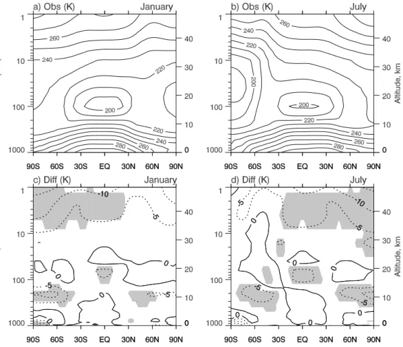
Figure 2 presents a comparison of latitude-pressure cross-sections of simulated and UKMO zonal mean temperatures for January and July. The evaluation of the
tem-10
perature distribution reveals that in the lower stratosphere the general agreement of the location and magnitude of the simulated extremes is rather good. SOCOL repro-duces the main observed features of zonal mean temperature distribution well: warm troposphere, cold tropical tropopause without apparent bias, cold winter middle strato-sphere, warm summer stratopause, and the polar temperature minimum associated
15
with the formation of the polar vortices.
4.1.2. Model/observation difference fields
A simple visual comparison of temperature and zonal wind fields has often been used to validate CCMs (e.g. Takigawa et al., 1999; Hein et al., 2001). From this kind of comparison one can only conclude how well a model reproduces the main observed
20
features of the zonal mean temperature and zonal mean zonal wind structures in gen-eral. However, differences between simulated and observed fields do exist and it is very helpful to use a more quantitative analysis of model deviations from observations as it has been presented by Rozanov et al. (2001) and Jonsson et al. (2002). Due to noticeable discrepancies among the available reanalysis data (e.g. SPARC, 2002) it
25
ACPD
5, 509–555, 2005Chemistry-climate model SOCOL
T. Egorova et al.
Title Page
Abstract Introduction
Conclusions References
Tables Figures
◭ ◮
◭ ◮
Back Close
Full Screen / Esc
Print Version Interactive Discussion
EGU
temperature (see Fig. 4a, b) and the standard deviation of these quantities described in Sect. 3. From the results of the 40-year long SOCOL integration we have also calcu-lated the climatology of the zonal wind (see Fig. 1a, b) and temperature (see Fig. 2a, b) and their standard deviations. Using these data sets we have calculated the difference between simulated and observed climatology and estimated the statistical significance
5
of these deviations using the Student t-test.
Figure 3c, d and 4c, d show ensemble mean monthly mean deviations of the model from the observational data in January and July for zonal means of zonal wind and tem-perature accordingly. The gray spots mark the area where the model deviations from the observational data are statistically significant at the 95% confidence level. In the
10
zonal wind field these spots appear in the region of the extra tropical jets implying that SOCOL has a tendency to reproduce stronger (up to 5–10 m/s) jets in the troposphere. In July the model produces weaker (up to 10 m/s) easterlies in the upper stratosphere. Also significant deviations of simulated zonal mean zonal wind of up to 25 m/s can be seen over 30◦S–60◦S in July, suggesting that the meridional gradient of temperature
15
in the model is too weak. All other deviations appear not to be statistically signifi-cant. In the temperature field (Fig. 4c, d) the model substantially deviates from the observational data near the tropopause and in the upper stratosphere of the summer hemisphere in high and middle latitudes. At the tropical tropopause and winter high lat-itude tropopause the discrepancies between simulated and observed data reach about
20
−6 K and in the summer hemisphere tropopause the deviation is up to −10 K. There are also statistically significant deviations in the upper stratosphere over the summer hemisphere high latitudes of up to 10 K. All deviations are negative, showing that the model is cold biased relative to the data.
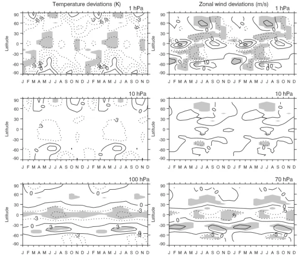
Figure 5 shows the seasonal variation of the simulated temperature (left panel) and
25
ACPD
5, 509–555, 2005Chemistry-climate model SOCOL
T. Egorova et al.
Title Page
Abstract Introduction
Conclusions References
Tables Figures
◭ ◮
◭ ◮
Back Close
Full Screen / Esc
Print Version Interactive Discussion
EGU
wind at 10 hPa deviates in the middle latitudes of the Southern Hemisphere (SH) dur-ing summer, however, the deviations do not exceed 5 m s−1. At 1 hPa a statistically significant cold bias of about 9 K has been found in January and February over south-ern high latitudes, in May, June and November at the equator, and of about 6 K over the high latitudes in the Northern Hemisphere (NH) in June and July. The positive
de-5
viations over the high latitudes in both hemispheres are not significant. At 100 hPa the model has a cold bias at the equator of up to 6 K and warm bias of up to 3 K in the extra tropical area during the boreal summer. The zonal wind deviation at 70 hPa is about ±5 ms−1in the tropical and southern middle latitudes.
4.1.3. Summary
10
From the zonal mean and seasonal variation analysis of zonal wind and temperature we conclude that during warm seasons our model does not have enough heating at high latitudes and at the equator. This might be connected to the problem in radia-tion code of MA-ECHAM4, which describes the absorpradia-tion of solar UV radiaradia-tion by ozone and oxygen with a rather simplified scheme. We will return to this problem
15
in Sect. 5. The temperature differences are most pronounced near the tropopause. These model deficiencies can be explained by the rough vertical model resolution in the upper troposphere-lower stratosphere (E. Roeckner, presentation on COSMOS workshop, Hamburg, May, 2003).
4.2. Chemical aspects of the validation
20
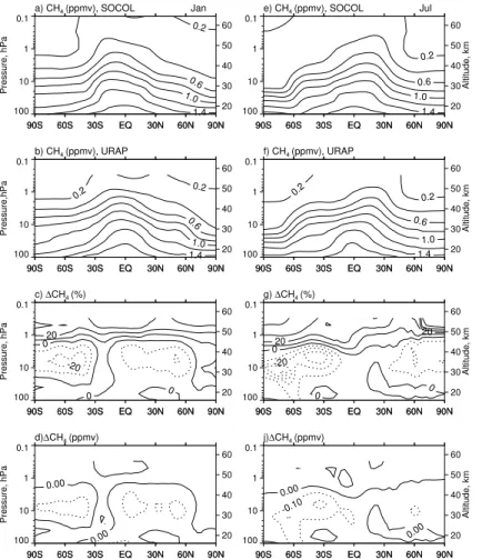
4.2.1. Methane
Altitude dependence.Methane is the most abundant hydrocarbon in the atmosphere and useful as a tracer of atmospheric circulation because of its long photochemical lifetime. Hence, the methane distribution is determined mainly by features of the circu-lation. Figure 6 shows the meridional cross section of the CH4mixing ratio climatology
ACPD
5, 509–555, 2005Chemistry-climate model SOCOL
T. Egorova et al.
Title Page
Abstract Introduction
Conclusions References
Tables Figures
◭ ◮
◭ ◮
Back Close
Full Screen / Esc
Print Version Interactive Discussion
EGU
simulated by SOCOL and observed by UARS together with their difference. The over-all zonal mean distribution (CH4 decreases with height and latitude) is similar to the
observed one and the agreement is within∼10–20% in the stratosphere. As a result of the transport by Brewer-Dobson circulation the tropical maxima of CH4 concentration is shifted to the North during boreal summer and to the South during boreal winter.
5
The subtropical transport barrier is also well simulated. The model reproduces down-ward motion over the poles but slightly too intensively and, therefore, at 10 hPa a 20% (∼0.1 ppmv) underestimation of the average CH4mixing ratio occurs.
Seasonal cycle. Latitude-time variations in the observed and simulated zonal av-erage mixing ratio of CH4 at 25 hPa are shown in Fig. 7. The model reproduces the
10
seasonal variation, which is similar to the HALOE data with a relative minimum over the high latitudes during December-February for the NH and September-November for the SH, while in the tropical area there is no apparent seasonal cycle. At 25 hPa the diff er-ence between simulated and observed data in the tropics and northern high latitudes is about 5% and in the southern high latitudes the difference reaches about 15%
be-15
cause of a half month shift of the minimum methane mixing ratio due to an unidentified reason.
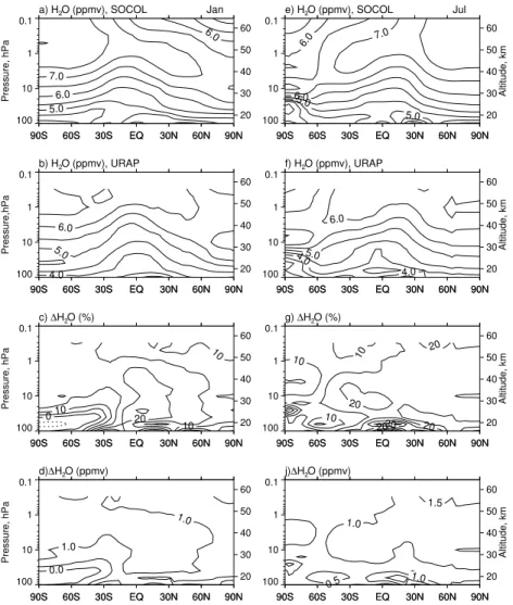
4.2.2. Water vapor
Altitude dependence. Water vapor is an important tracer in the upper troposphere and lower stratosphere. In both regions H2O is a source of HOx radicals, which are
20
involved in photosmog reactions producing ozone in the upper troposphere and in catalytic ozone destruction cycles in the stratosphere. Figure 8 presents meridional cross-sections of water vapor mixing ratios. The zonal-mean distribution of H2O is well
reproduced by SOCOL. However, the model overestimates mixing ratio of H2O com-pared to URAP data in the stratosphere by 0.5–1.0 ppmv (or 10–20%), which is within
25
up-ACPD
5, 509–555, 2005Chemistry-climate model SOCOL
T. Egorova et al.
Title Page
Abstract Introduction
Conclusions References
Tables Figures
◭ ◮
◭ ◮
Back Close
Full Screen / Esc
Print Version Interactive Discussion
EGU
ward branch of the Brewer-Dobson circulation, which determines vertical transport and on the H2O mixing ratio at the entry level. Figure 6 shows a small underestimation of CH4mixing ratios in the middle stratosphere, which implies that the vertical transport in
our model is just slightly underestimated, therefore the overestimation of stratospheric H2O is more likely connected to the overestimated H2O mixing ratio at the entry level
5
of the model.
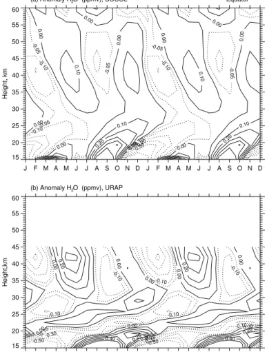
Seasonal cycle.The seasonal variation of simulated H2O mixing ratios at 10 hPa is
compared with URAP data in Fig. 9. The model and URAP data do not show a suffi -ciently strong annual cycle in the tropical middle stratosphere. Over the high latitudes both model and observations reveal elevated H2O mixing ratios during wintertime,
as-10
sociated with aged air with low CH4descending into the polar vortices.
Figure 10 presents a comparison of the simulated and URAP-derived data set of the altitude-time anomaly in the H2O mixing ratio (deviation from annual mean) over the
equator. The model reproduces the vertical propagation of the dry (negative) and wet (positive) anomalies induced by the water vapor changes in the lower stratosphere, i.e.
15
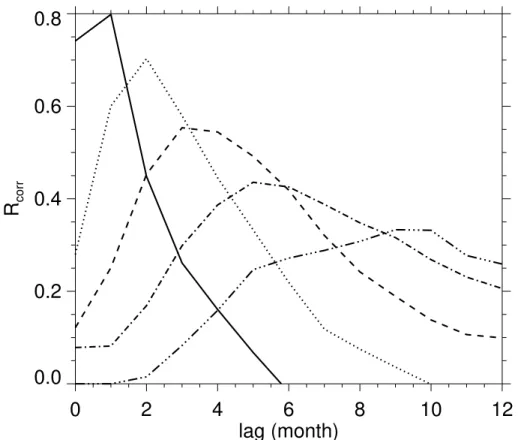
water vapor “tape recorder” described by Mote et al. (1998). However, the model up-ward transport is up to twice as fast as observed. In order to quantitatively estimate the intensity of the upward water vapor transport we have calculated lagged correlations between deseasonalized H2O mixing ratio anomalies at 16 km altitude and at diff
er-ent altitudes in the equatorial stratosphere. The correlation coefficients are plotted in
20
Fig. 11 for the 19.4, 22.7, 25.9, 29.1 and 32.3 km levels. The time when the maximum correlation is reached and the distance between levels allow the estimation of the verti-cal velocities in the equatorial lower stratosphere. For the plotted data the mean vertiverti-cal velocity between 16 and 32.3 km is equal to∼0.6 mm/s, which exceeds the value ob-tained from the observed H2O distribution by about 50–90%. The vertical velocity is
25
ACPD
5, 509–555, 2005Chemistry-climate model SOCOL
T. Egorova et al.
Title Page
Abstract Introduction
Conclusions References
Tables Figures
◭ ◮
◭ ◮
Back Close
Full Screen / Esc
Print Version Interactive Discussion
EGU
In the upper stratosphere the model quantitatively matches the observed semi-annual oscillation with positive anomalies during the boreal summer (Fig. 10).
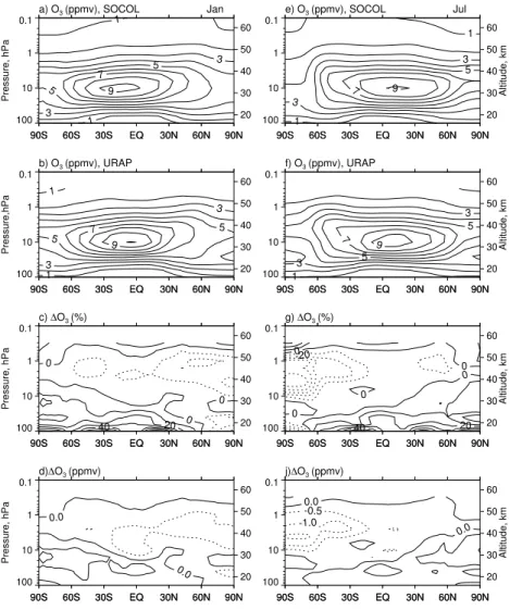
4.2.3. Ozone
Altitude dependence. Figure 12 presents meridional cross sections of zonal mean monthly mean O3mixing ratios, simulated by SOCOL and observed by UARS together
5
with their difference. The distribution of the simulated ozone is in good agreement with the observations throughout the stratosphere where the model errors remain basically within±10%. The simulated maximum of the zonal mean (∼9 ppmv) appears at the equator, at around 10 hPa, which is consistent with the observations. The so-called “banana” shape of the ozone distribution is also well captured by the model with high
10
ozone regions extending to the upper polar stratosphere. The model substantially un-derestimates ozone over the southern high latitudes in the upper stratosphere during the austral winter season. The cause of the ozone underestimation could be related to (or identical to) the causes as for the underestimation of methane and the overestima-tion of water vapor in the same region: this could stem from a too strong isolaoverestima-tion of
15
the southern polar vortex and a too strong downward transport in the simulation. The fact that methane is longer-lived than ozone in these regions could be the reason for the methane discrepancy appearing only at lower altitudes.
Seasonal cycle. The comparison of the seasonal variation of the simulated to-tal ozone column (TOC) with the observations is presented in Fig. 13. There are
20
no gaps during polar nights in the observations because the observed total ozone fields are the composite of the available satellite data for 1993–2002, which include the infrared-based TOVS data. SOCOL reproduces a seasonal maximum in the NH and a maximum and minimum in the SH with reasonable accuracy. The overall agreement between the model and the observation data composite is within±5% in the tropics,
25
ACPD
5, 509–555, 2005Chemistry-climate model SOCOL
T. Egorova et al.
Title Page
Abstract Introduction
Conclusions References
Tables Figures
◭ ◮
◭ ◮
Back Close
Full Screen / Esc
Print Version Interactive Discussion
EGU
satellite observations. The position and magnitude of the ozone ‘hole’ is very well re-produced by SOCOL, implying that the amount of PSCs during the spring season and chemical ozone destruction are reasonably well captured by the chemical routine of the model. The position of the total ozone maximum in the Australian sector is also well captured by SOCOL, however the magnitude of the maximum is slightly
underes-5
timated (by about 8 DU or∼2%). Some CCMs (see Austin et al., 2003, their Fig. 2) substantially overestimate the magnitude of the total ozone maxima over the middle latitudes in the Australian sector. This could imply that the relevant wave forcing and subsequently meridional transport in these models are too strong, but SOCOL seems not to suffer from this problem.
10
We have compared the pattern correlation and absolute deviation (not shown) of total ozone simulated by SOCOL and simulated by CCMs that participated in the model intercomparison presented by (Austin et al., 2003). The comparison shows that among the other models SOCOL has the smallest absolute deviation from the observations in the SH, which is∼2% and very high pattern correlation (more than 0.95) over both
15
hemispheres. Over the Northern Hemisphere SOCOL underestimates the total ozone maximum in March by about 75 DU, but nevertheless has one of the smallest absolute deviations (∼5%) of total ozone over NH from the observational data among the models compared by Austin et al. (2003).
4.3. Sensitivity of ozone and temperature to the strength of the Arctic winter vortex
20
The aim of this particular exercise is to validate the ability of SOCOL to simulate the imprint of the Arctic Oscillation (AO) in stratospheric ozone and temperature during the boreal winter. It is well known that the positive phase of the AO is characterized by a deeper vortex and a more intensive Polar Night Jet (e.g. Thompson and Wallace, 1998). Therefore, it is theoretically expected (e.g. Kodera and Kuroda, 2002) that the
25
ACPD
5, 509–555, 2005Chemistry-climate model SOCOL
T. Egorova et al.
Title Page
Abstract Introduction
Conclusions References
Tables Figures
◭ ◮
◭ ◮
Back Close
Full Screen / Esc
Print Version Interactive Discussion
EGU
compare them.
To analyze this process a 25-year long simulation of the present day atmosphere with the CCM SOCOL has been used. We divided the simulated data into two groups according to the intensity of the polar vortex during the boreal winter season defined by the anomaly of North Pole geopotential height at 100 hPa and contrasted the difference
5
between these two groups against observational data processed in an identical way. The observations we used are NMC data (for 1978–1998) and SAGE I/II ozone density (for 1979–2001) compiled by W. Randel et al. (http://www.acd.ucar.edu/∼randel).
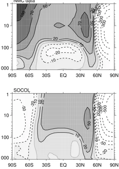
Figures 15–18 illustrate the differences between the two groups mentioned above, in zonal mean geopotential height, zonal wind, temperature and ozone mixing ratio
aver-10
aged over the boreal winter season (December-January-February). Figure 15 shows that the simulated and observed differences in geopotential heights are broadly similar in the NH and tropical stratosphere. The deepening of the polar vortex and formation of the ridges over mid-latitudes is clearly visible for the positive AO phase in both data sets. The zonal wind difference in the composite (Fig. 16) consists of an
accelera-15
tion of the PNJ by 10–15 m s−1 in the simulated and observed data. The changes of zonal wind in the rest of the atmosphere are rather small. Figure 17 demonstrates the pattern of the temperature response. The simulated and observed temperature re-sponses over the NH are similar and consist of a pronounced dipole-like structure with cooling (warming) in the middle-lower (upper) stratosphere. In the tropics, the model
20
matches the warming in the lower stratosphere, although the magnitude of the simu-lated warming is about 2 times smaller. The model is unable to capture warming in the upper tropical stratosphere. The simulated dipole-like temperature changes are at a higher altitude than the observed temperature changes. The ozone response is shown in Fig. 18. The simulated and observed changes are in qualitative agreement only in
25
ACPD
5, 509–555, 2005Chemistry-climate model SOCOL
T. Egorova et al.
Title Page
Abstract Introduction
Conclusions References
Tables Figures
◭ ◮
◭ ◮
Back Close
Full Screen / Esc
Print Version Interactive Discussion
EGU
transport and is consistent with temperature and zonal wind changes. However, it is not so clearly visible in the observational data analysis.
5. Conclusions
In this paper we presented a description of a new modeling tool, the CCM SOCOL, together with the validation of the simulated present-day climatology against a variety
5
of observational data. We also present an example of processes-oriented validation. While the model performance is quite satisfactory based on an overall inspection of simulated fields and on a proper statistical analysis, we have identified a number of weaknesses in the model that need to be addressed for the future improvement of the model. In particular, the analysis of the simulated zonal wind and temperature
10
deviations shows that for an improvement it will be necessary to pay special attention to the tropopause region in the tropics and at high latitudes as well as to the description of the processes in the upper stratosphere and mesosphere, where significant cold biases have been found in the model during boreal summer.
The model’s too cold upper stratosphere is most likely related to the radiation code
15
of MA-ECHAM4 (see Sect. 4), which does not take into account the absorption of the solar irradiance for the wavelengths shorter than 250 nm. To illustrate the importance of this spectral region we have applied a 1-D radiative convective model (RCM) de-scribed by Rozanov et al. (2002b) and calculated the temperature profiles with and without absorption of the solar irradiance in the spectral region 120–250 nm.
Temper-20
ature differences due to absorption of the solar irradiance in the 120–250 nm spectral interval have been calculated with the 1-D RCM for three cases: (1) a tropical atmo-sphere model, with Solar Zenith Angle (SZA)=45◦, duration of the day (DoD)=12 h; (2) a middle latitude summer atmosphere model, with SZA=60◦, DoD=14.4 h; (3) a subarc-tic summer atmosphere model, with SZA=70◦, DoD=24 h. The results are depicted in
25
ACPD
5, 509–555, 2005Chemistry-climate model SOCOL
T. Egorova et al.
Title Page
Abstract Introduction
Conclusions References
Tables Figures
◭ ◮
◭ ◮
Back Close
Full Screen / Esc
Print Version Interactive Discussion
EGU
the heat would substantially improve temperature and zonal wind distributions in the summer extra-tropical upper stratosphere and mesosphere also in the 3-D model.
The simulated descent of the air is too strong in the polar stratosphere, leading to a significant underestimation of CH4 and O3 mixing ratios in this area. The tropopause
region is cold biased by 5–10 K, which might be related to an insufficient vertical
res-5
olution. An analysis of the water vapor zonal mean and seasonal distributions reveals an overestimation of stratospheric H2O, which is probably related to the transport of
H2O from the troposphere.
As a process-oriented part of the validation we analyzed how SOCOL reproduces the imprint of the AO onto the temperature and ozone fields. During the boreal winter
10
(DJF) a signature of the positive AO phase or strong northern polar vortex is clearly visible in the observed and simulated data. Therefore the applied approach can be used for the validation of CCMs. SOCOL reasonably well reproduces AO-like patterns of the inter-annual variability, which consist of a deepening of the polar vortex and an acceleration of the PNJ during positive AO phases. The model also captures the
con-15
comitant deceleration of the meridional circulation, the subsequent warming, and the ozone increase in the lower tropical stratosphere. The model also matches the pro-nounced dipole-like temperature response over the northern high-latitudes. However, the simulated warming in the tropical lower stratosphere is underestimated by a fac-tor of 2. In the upper stratosphere the model almost completely fails to reproduce the
20
observed warming. The observed ozone response in the tropical lower stratosphere is confined mostly to the lowermost stratosphere while the simulated ozone response extends to the middle stratosphere. Moreover, the ozone response over the northern high-latitudes disagrees with observed ozone changes. Additional observation and simulation data should be analyzed in order to elucidate the causes of the noticeable
25
ACPD
5, 509–555, 2005Chemistry-climate model SOCOL
T. Egorova et al.
Title Page
Abstract Introduction
Conclusions References
Tables Figures
◭ ◮
◭ ◮
Back Close
Full Screen / Esc
Print Version Interactive Discussion
EGU
performance. Thus, many research groups can use it for studies of chemistry-climate problems even without access to large super-computer facilities.
Software availability
Name of the software: Modeling tool for studies Solar Climate Ozone links (SOCOL)
5
Developer and contact address: PMOD/WRC and IAC ETH, Zurich, Dorfstrasse, 33, CH-7260, Davos Dorf, Switzerland
Telephone and fax: tel.+41 081 4175138, fax. +41 081 4175100
10
E-mail: [email protected]
Hardware required: Intel Pentium based PC, 512 MB memory at least
Software required: LINUX, Fujitsu/Lahey FORTRAN
15
Availability and cost: signed Max Planck Institute for Meteorology Software License Agreement (http://www.mpimet.mpg.de/en/extra/models/distribution/ mpi-m sla 200403.pdf), appropriate citation required, collaboration preferable, free of charge.
20
Acknowledgements. This paper is based upon work supported by the by the Swiss Federal Institute of Technology, Z ¨urich and PMOD/WRC, Davos, Switzerland. The work of V. Zubov was supported by INTAS (grant INTAS-01-0432) and RFFI (grant 02-05-65399). We thank the SPARC, URAP and TOMS Data Centers for providing the data and C. Hoyle and P. Forney for editing the manuscript.
ACPD
5, 509–555, 2005Chemistry-climate model SOCOL
T. Egorova et al.
Title Page
Abstract Introduction
Conclusions References
Tables Figures
◭ ◮
◭ ◮
Back Close
Full Screen / Esc
Print Version Interactive Discussion
EGU References
Austin, J., Shindell, D., Beagley, S. R., et al.: Uncertainties and assessments of chemistry-climate models of the stratosphere, Atmos. Chem. Phys., 3, 1–27, 2003,
SRef-ID: 1680-7324/acp/2003-3-1.
Baldwin, M.: The Arctic Oscillation and its role in stratosphere-troposphere coupling, SPARC
5
newsletter no
14, 10–14, 2000.
Br ¨onnimann, S., Luterbacher, J., Staehelin, J., and Svendby, T.: An extreme anomaly in stratospheric ozone over Europe in 1940–1942, Geophys. Res. Lett., 31, L08101, doi:10.1029/2004GL019611, 2004.
Butchart, N. and Austin, J.: On the relationship between the quasi-biennial oscillation, total
10
chlorine and the severity of the Antarctic ozone hole, Q. J. R. Meteorol. Soc., 122, 183–217, 1996.
Butchart, N. and Austin, J.: Middle Atmosphere Climatologies from the Troposphere-Stratosphere Configuration of the UKMO’s Unified Model, J. Atmos. Sci., 35, 2782–2809, 1998.
15
Carslaw, K. S., Luo, B. P., and Peter, Th.: An analytic expression for the composition of aqueous HNO3-H2SO4stratospheric aerosols including gas phase removal of HNO3, Geophys. Res. Lett., 22, 1877–1880, 1995.
Charron, M. and Manzini, E.: Gravity waves from fronts: Parameterization and middle atmo-sphere response in a general circulation model, J. Atmos. Sci., 59, 923–941, 2002.
20
DeMore, W. B., Sander, S. P., Golden, D. M., Hampson, R. F., Kurylo, M. J., Howard, C. J., Ravishankara, A. R., Kolb, C. E., and Molina, M. J.: Chemical Kinetics and Photochemical Data for Use in Stratospheric Modeling, Evaluation 12, JPL Publication, 97-4, 1997.
Egorova, T. A., Rozanov, E. V., Schlesinger, M. E., Andronova, N. G., Malyshev, S. L., Zubov, V. A., and Karol, I. L.: Assessment of the effect of the Montreal Protocol on atmospheric ozone,
25
Geophys. Res. Lett., 28, 2389–2392, 2001.
Egorova, T. A., Rozanov, E. V., Zubov, V. A., and Karol, I. L.: Model for Investigating Ozone Trends (MEZON), Izvestiya, Atmospheric and Oceanic Physics, 39, 277–292, 2003.
Egorova, T., Rozanov, E., Manzini, E., Haberreiter, M., Schmutz, W., Zubov, V., and Peter, T.: Chemical and dynamical response to the 11-year variability of the solar
ir-30
ACPD
5, 509–555, 2005Chemistry-climate model SOCOL
T. Egorova et al.
Title Page
Abstract Introduction
Conclusions References
Tables Figures
◭ ◮
◭ ◮
Back Close
Full Screen / Esc
Print Version Interactive Discussion
EGU
Eyring, V., Harris, N., Rex, M., et al.: Comprehensive Summary on the Workshop on “Process-Oriented Validation of Coupled Chemistry-Climate Models”, SPARC, Newsletter, 23, 5–11, 2004.
Fouquart, Y. and Bonnel, B.: Computations of solar heating of the Earth’s atmosphere: A new parameterization, Beitr. Phys. Atmos., 53, 35–62, 1980.
5
Gleckler, P. E.: AMIP Newsletter: AMIP-II guidelines, Lawrence Livermore Natl. Lab, Livermore, Calif., 1996.
Hanson, D. and Maursberger, K.: Laboratory studies of the nitric acid trihydrate: Implications for the south polar stratosphere, Geophys. Res. Lett., 15, 855–858, 1988.
Harries, J. E., Tuck, A. F., Gordley, L. L., et al.: Validation of measurements of water vapor from
10
the halogen occultation experiment (HALOE), J. Geophys. Res., 101 (D6), 10 205–10 216, 1996.
Hein, R., Dameris, M., Schnadt, C., and Coauthors: Results of an interactively coupled atmo-spheric chemistry – general circulation model: Comparison with observations, Ann. Geo-phys., 19, 435–457, 2001,
15
SRef-ID: 1432-0576/ag/2001-19-435.
Hines, C. O.: Doppler spread parameterization of gravity wave momentum deposition in the middle atmosphere, 1, Basic formulation, J. Atmos. Solar Terr. Phys., 59, 371–386, 1997a. Hines, C. O.: Doppler spread parameterization of gravity wave momentum deposition in the
middle atmosphere, 2, Broad and quasi monochromatic spectra and implementation, J.
At-20
mos. Solar Terr. Phys., 59, 387–400, 1997b.
Intergovernmental Panel of Climate Change: Climate Change 2001: The Scientific Basis, Cam-bridge Univ. Press, New York, 881, 2001.
Jacobson, M. Z. and Turco, R. P.: SMVGEAR: A sparse-matrix, vectorized code for atmospheric models, Atmos. Environ., 28, 273–284, 1994.
25
Jonsson, A., de Grandpre, J., and McConnell, J. C.: A comparison of mesospheric tempera-tures from the Canadian Middle Atmospheric Model and HALOE observations: Zonal mean and signature of the solar diurnal tide, Geophys. Res. Lett., 29, doi:10.1029/2001GL014476, 2002.
Kodera, K. and Kuroda, Y.: Dynamical response to the solar cycle, J. Geophys. Res., 107 (D24),
30
4749, doi:10.1029/2002JD002224, 2002.
ACPD
5, 509–555, 2005Chemistry-climate model SOCOL
T. Egorova et al.
Title Page
Abstract Introduction
Conclusions References
Tables Figures
◭ ◮
◭ ◮
Back Close
Full Screen / Esc
Print Version Interactive Discussion
EGU
31 523–31 539, 1998.
Manzini, E., McFarlane, N. A., and McLandress, C.: Impact of the Doppler Spread Parameteri-zation on the simulation of the middle atmosphere circulation using the MA/ECHAM4 general circulation model, J. Geophys. Res., 102, 25 751–25 762, 1997.
McFarlane, N. A.: The effect of orographically exited gravity wave drag on the general circulation
5
of the lower stratosphere and troposphere, J. Atmos. Sci., 44, 1775–1800, 1987.
Morcrette, J. J.: Radiation and cloud radiative properties in the European Center for Medium-Range Weather Forecasts forecasting system, J. Geophys. Res., 96, 9121–9132, 1991. Mote, P. W., Dunkerton, T. J., McIntyre, M. E., Ray, E. A., Haynes, P. H., and Russell, J.
M.: Vertical velocity, vertical diffusion, and dilution by midlatitude air in the tropical lower
10
stratosphere, J. Geophys. Res., 103, 8651–8666, 1998.
Nagashima, T., Takahashi, M., Takigawa, M., and Akiyoshi, H.: Future development of the ozone layer calculated by a general circulation model with fully interactive chemistry, Geo-phys. Res. Lett., 29, doi:10.1029/2001GL014026, 2002.
Pawson, S., Kodera, K., Hamilton, K., et al.: The GCM-reality intercomparison project for
15
SPARC (GRIPS): Scientific issues and initial results, Bull. Amer. Meteor. Soc., 81, 781–796, 2000.
Prather, M. J.: Numerical Advection by Conservation of Second-Order Moments, J. Geophys. Res., 91, 6671–6681, 1986.
Roeckner, E., Arpe, K., Bengtsson, L., Christoph, M., Claussen, M., D ¨umenil, L., Esch, M.,
20
Giorgetta, M., Schlese, U., and Schulzweida, U.: The atmospheric general circulation model ECHAM4: Model description and simulation of the present day climate, Tech. Rep. 218, Max Planck Ins. for Meteorol., Hamburg, Germany, 1996a.
Roeckner, E., Oberuber, J. M., Bacher, A., Christoph, M., and Kirchner, I.: ENSO variability and atmospheric response in a global coupled atmosphere-ocean GCM, Clim. Dynamics.,
25
12, 734–754, 1996b.
Rozanov, E. V., Schlesinger, M. E., Zubov, V. A., Yang, F., and Andronova, N. G.: The UIUC three-dimensional stratospheric chemical transport model: Description and evaluation of the simulated source gases and ozone, J. Geophys. Res., 104, 11 755–11 781, 1999.
Rozanov, E. V., Schlesinger, M. E., and Zubov, V. A.: The University of Illinois,
Urbana-30
ACPD
5, 509–555, 2005Chemistry-climate model SOCOL
T. Egorova et al.
Title Page
Abstract Introduction
Conclusions References
Tables Figures
◭ ◮
◭ ◮
Back Close
Full Screen / Esc
Print Version Interactive Discussion
EGU
Rozanov, E. V., Schlesinger, M. E., Andronova, N. G., Yang, F., Malyshev, S. L., Zubov, V. A., Egorova, T. A., and Li, B.: Climate/chemistry effects of the Pinatubo volcanic eruption simulated by the UIUC stratosphere/troposphere GCM with interactive photochemistry, J. Geophys. Res., 107 (D21), 4594, doi:10.1029/2001JD000974, 2002a.
Rozanov, E., Egorova, T., Fr ¨ohlich, C., Haberreiter, M., Peter, T., and Schmutz, W.: Estimation
5
of the ozone and temperature sensitivity to the variation of spectral solar flux, In: “From Solar Min to Max: Half a Solar Cycle with SOHO”, ESA SP-508, 181–184, 2002b.
Rozanov, E. V., Schlesinger, M. E., Egorova, T. A., et al.: Atmospheric Response to the Observed Increase of Solar UV Radiation from Solar Minimum to Solar Maximum Simulated by the UIUC Climate-Chemistry Model, J. Geophys. Res., 109, D01110,
10
doi:10.1029/2003JD003796, 2004.
Sander, S. P., Friedl, R. R., DeMore, W. B., Golden, D. M., Hampson, R. F., Kurylo, M. J., Huie, R. E., Moortgat, G. K., Ravishankara, A. R., Kolb, C. E., and Molina, M. J.: Chemical Kinetics and Photochemical Data for Use in Stratospheric Modeling: Supplement to Evaluation 12: Update of Key Reactions, Evaluation 13, JPL Publication, 2000.
15
Sherman, A. H. and Hindmarsh, A. C.: GEARS: A package for the solution of sparse stiff, ordinary differential equations, Lawrence Livermore Lab. Rep. UCID-30114, 1980.
Shindell, D. T., Rind, D., and Lonergan, P.: Increased polar stratospheric ozone losses and delayed eventual recovery owing to increasing greenhouse-gas concentrations, Nature, 392, 589–592, 1998.
20
Schnadt, C., Dameris, M., Ponater, M., Hein, R., Grewe, V., and Steil, B.: Interaction of atmo-spheric chemistry and climate and its impact on stratoatmo-spheric ozone, Clim. Dynamics., 18, 507–517, 2002.
SPARC: SPARC Intercomparison of Middle Atmosphere Climatologies, SPARC Rep. 3, 96, 2002.
25
Steil, B., Bruhl, C., Manzini, E., et al.: A new interactive chemistry-climate model: 1. Present-day climatology and interannual variability of the middle atmosphere using the model and 9 years of HALOE/UARS data, J. Geophys. Res., 108 (D9), 4290, doi:10.1029/2002JD002971, 2003.
Swinbank, R. and Ortland, D. A.: Compilation of wind data for the UARS Reference Atmosphere
30
Project, J. Geophys. Res., 108 (D19), 4615, doi:10.1029/2002JD003135, 2003.
ACPD
5, 509–555, 2005Chemistry-climate model SOCOL
T. Egorova et al.
Title Page
Abstract Introduction
Conclusions References
Tables Figures
◭ ◮
◭ ◮
Back Close
Full Screen / Esc
Print Version Interactive Discussion
EGU
atmospheric GCM with coupled stratospheric chemistry, J. Geophys. Res., 104, 14 003– 14 018, 1999.
Thompson, D. and Wallace, J.: The arctic oscillation signature in the wintertime geopotential height and temperature fields, Geophys. Res. Lett., 25, 1297–1300, 1998.
Zubov, V., Rozanov, E., and Schlesinger, M.: Hybrid scheme for tree-dimensional advective
5
transport, Mon. Wea. Rev., 127, 1335–1346, 1999.
ACPD
5, 509–555, 2005Chemistry-climate model SOCOL
T. Egorova et al.
Title Page
Abstract Introduction
Conclusions References
Tables Figures
◭ ◮
◭ ◮
Back Close
Full Screen / Esc
Print Version Interactive Discussion
EGU
Table 1.Climatological data sets used for model validation.
ACPD
5, 509–555, 2005Chemistry-climate model SOCOL
T. Egorova et al.
Title Page
Abstract Introduction
Conclusions References
Tables Figures
◭ ◮
◭ ◮
Back Close
Full Screen / Esc
Print Version Interactive Discussion
EGU
Fig. 1. Meridional cross-section of the zonal mean zonal wind (ms−1
ACPD
5, 509–555, 2005Chemistry-climate model SOCOL
T. Egorova et al.
Title Page
Abstract Introduction
Conclusions References
Tables Figures
◭ ◮
◭ ◮
Back Close
Full Screen / Esc
Print Version Interactive Discussion
EGU
Fig. 2.Same as Fig. 1 but for the zonal mean temperature (K). Observed values are from the
ACPD
5, 509–555, 2005Chemistry-climate model SOCOL
T. Egorova et al.
Title Page
Abstract Introduction
Conclusions References
Tables Figures
◭ ◮
◭ ◮
Back Close
Full Screen / Esc
Print Version Interactive Discussion
EGU
Fig. 3.Zonal mean zonal wind climatology of composite data(a, b)(contours via 10 ms−1) and
difference (contours via 5 ms−1
ACPD
5, 509–555, 2005Chemistry-climate model SOCOL
T. Egorova et al.
Title Page
Abstract Introduction
Conclusions References
Tables Figures
◭ ◮
◭ ◮
Back Close
Full Screen / Esc
Print Version Interactive Discussion
EGU
ACPD
5, 509–555, 2005Chemistry-climate model SOCOL
T. Egorova et al.
Title Page
Abstract Introduction
Conclusions References
Tables Figures
◭ ◮
◭ ◮
Back Close
Full Screen / Esc
Print Version Interactive Discussion
EGU
Fig. 5. Deviations of the simulated temperature and zonal wind seasonal variation from the
ACPD
5, 509–555, 2005Chemistry-climate model SOCOL
T. Egorova et al.
Title Page Abstract Introduction Conclusions References Tables Figures ◭ ◮ ◭ ◮ Back Close
Full Screen / Esc
Print Version Interactive Discussion
EGU
90S 60S 30S EQ 30N 60N 90N 100 10 1 0.1 Pressure, hPa 0.2 0.6 1.0 1.4 a) CH4 (ppmv), SOCOL Jan
90S 60S 30S EQ 30N 60N 90N 20 30 40 50 60
90S 60S 30S EQ 30N 60N 90N 100 10 1 0.1 Pressure,hPa 0.2 0.2 0.6 1.0 1.4 b) CH4 (ppmv), URAP
90S 60S 30S EQ 30N 60N 90N 20 30 40 50 60
90S 60S 30S EQ 30N 60N 90N 100 10 1 0.1 Pressure, hPa -20 0 0 0 20 c) ∆CH4 (%)
90S 60S 30S EQ 30N 60N 90N 20 30 40 50 60
90S 60S 30S EQ 30N 60N 90N 100 10 1 0.1 Pressure, hPa 0.00 0.00
d)∆CH4 (ppmv)
90S 60S 30S EQ 30N 60N 90N 20 30 40 50 60
90S 60S 30S EQ 30N 60N 90N 100 10 1 0.1 0.2 0.6 1.0 1.4 e) CH4 (ppmv), SOCOL Jul
90S 60S 30S EQ 30N 60N 90N 20 30 40 50 60 Altitude, km
90S 60S 30S EQ 30N 60N 90N 100 10 1 0.1 0.2 0.2 0.6 1.0 1.4 f) CH4 (ppmv), URAP
90S 60S 30S EQ 30N 60N 90N 20 30 40 50 60 Altitude, km
90S 60S 30S EQ 30N 60N 90N 100 10 1 0.1 -20 0 0 0 20 20 g) ∆CH4 (%)
90S 60S 30S EQ 30N 60N 90N 20 30 40 50 60 Altitude, km
90S 60S 30S EQ 30N 60N 90N 100
10 1 0.1
j)∆CH4 (ppmv)
-0.10
0.00
0.00
90S 60S 30S EQ 30N 60N 90N 20 30 40 50 60 Altitude, km
Fig. 6. Latitude-pressure cross-section of the CH4 (ppmv) for January (left panel) and July
ACPD
5, 509–555, 2005Chemistry-climate model SOCOL
T. Egorova et al.
Title Page
Abstract Introduction
Conclusions References
Tables Figures
◭ ◮
◭ ◮
Back Close
Full Screen / Esc
Print Version Interactive Discussion
EGU
Fig. 7. Seasonal variation of methane at 25 hPa: (a) simulated, (b) observed, and(c) their
ACPD
5, 509–555, 2005Chemistry-climate model SOCOL
T. Egorova et al.
Title Page Abstract Introduction Conclusions References Tables Figures ◭ ◮ ◭ ◮ Back Close
Full Screen / Esc
Print Version Interactive Discussion
EGU
90S 60S 30S EQ 30N 60N 90N 100 10 1 0.1 Pressure, hPa 5.0 6.0 6.0 7.0
a) H2 O (ppmv), SOCOL Jan
90S 60S 30S EQ 30N 60N 90N 20 30 40 50 60
90S 60S 30S EQ 30N 60N 90N 100 10 1 0.1 Pressure,hPa 4.0 5.0 6.0
b) H2 O (ppmv), URAP
90S 60S 30S EQ 30N 60N 90N 20 30 40 50 60
90S 60S 30S EQ 30N 60N 90N 100 10 1 0.1 Pressure, hPa 0 10 10 10 20 c) ∆H2 O (%)
90S 60S 30S EQ 30N 60N 90N 20 30 40 50 60
90S 60S 30S EQ 30N 60N 90N 100 10 1 0.1 Pressure, hPa 0.0 1.0 1.0
d)∆H2 O (ppmv)
90S 60S 30S EQ 30N 60N 90N 20 30 40 50 60
90S 60S 30S EQ 30N 60N 90N 100 10 1 0.1 5.0 5.0 6.0 6.0 7.0
e) H2 O (ppmv), SOCOL Jul
90S 60S 30S EQ 30N 60N 90N 20 30 40 50 60 Altitude, km
90S 60S 30S EQ 30N 60N 90N 100 10 1 0.1 4.0 4.0 5.0 6.0
f) H2 O (ppmv), URAP
90S 60S 30S EQ 30N 60N 90N 20 30 40 50 60 Altitude, km
90S 60S 30S EQ 30N 60N 90N 100 10 1 0.1 10 10 10 20 20 20 2030 g) ∆H2 O (%)
90S 60S 30S EQ 30N 60N 90N 20 30 40 50 60 Altitude, km
90S 60S 30S EQ 30N 60N 90N 100
10 1 0.1
j)∆H2 O (ppmv)
0.5 1.0
1.0
1.5
90S 60S 30S EQ 30N 60N 90N 20 30 40 50 60 Altitude, km
ACPD
5, 509–555, 2005Chemistry-climate model SOCOL
T. Egorova et al.
Title Page
Abstract Introduction
Conclusions References
Tables Figures
◭ ◮
◭ ◮
Back Close
Full Screen / Esc
Print Version Interactive Discussion
EGU
ACPD
5, 509–555, 2005Chemistry-climate model SOCOL
T. Egorova et al.
Title Page Abstract Introduction Conclusions References Tables Figures ◭ ◮ ◭ ◮ Back Close
Full Screen / Esc
Print Version Interactive Discussion
EGU
J F M A M J J A S O N D J F M A M J J A S O N D 15 20 25 30 35 40 45 50 55 60 Height, km
(a) Anomaly H2 O (ppmv), SOCOL Equator
-0.30-0.20 -0.10 -0.10 -0.10 -0.10 -0.05 -0.05 -0.05 -0.05 -0.05 -0.05 0.00 0.00 0.00 0.00 0.00 0.00 0.00 0.00 0.00 0.00 0.10 0.10 0.10 0.10 0.20 0.20
J F M A M J J A S O N D J F M A M J J A S O N D 15 20 25 30 35 40 45 50 55 60 Height,km
(b) Anomaly H2 O (ppmv), URAP
-0.50 -0.50 -0.30 -0.30 -0.10 -0.10 -0.10 -0.10 -0.10 -0.10 -0.10 -0.10 0.00 0.00 0.00 0.00 0.00 0.00 0.00 0.00 0.00 0.20 0.20 0.20 0.20 0.40 0.40
Fig. 10. Altitude-time evolution of water vapor mixing ratio anomaly over the equator, derived
ACPD
5, 509–555, 2005Chemistry-climate model SOCOL
T. Egorova et al.
Title Page
Abstract Introduction
Conclusions References
Tables Figures
◭ ◮
◭ ◮
Back Close
Full Screen / Esc
Print Version Interactive Discussion
EGU
0
2
4
6
8
10
12
lag (month)
0.0
0.2
0.4
0.6
0.8
R
corrFig. 11. Lagged correlation coefficients of deseasonalised H2O mixing ratio anomalies in the
ACPD
5, 509–555, 2005Chemistry-climate model SOCOL
T. Egorova et al.
Title Page Abstract Introduction Conclusions References Tables Figures ◭ ◮ ◭ ◮ Back Close
Full Screen / Esc
Print Version Interactive Discussion
EGU
90S 60S 30S EQ 30N 60N 90N 100 10 1 0.1 Pressure, hPa 1 1 3 3 5 5 7 9
a) O3 (ppmv), SOCOL Jan
90S 60S 30S EQ 30N 60N 90N 20 30 40 50 60
90S 60S 30S EQ 30N 60N 90N 100 10 1 0.1 Pressure,hPa 1 1 3 3 5 5 7 9 b) O3 (ppmv), URAP
90S 60S 30S EQ 30N 60N 90N 20 30 40 50 60
90S 60S 30S EQ 30N 60N 90N 100 10 1 0.1 Pressure, hPa 0 0 0 20 40
c) ∆O3 (%)
90S 60S 30S EQ 30N 60N 90N 20 30 40 50 60
90S 60S 30S EQ 30N 60N 90N 100 10 1 0.1 Pressure, hPa 0.0 0.0
d)∆O3 (ppmv)
90S 60S 30S EQ 30N 60N 90N 20 30 40 50 60
90S 60S 30S EQ 30N 60N 90N 100 10 1 0.1 1 1 3 3 5 7 9
e) O3 (ppmv), SOCOL Jul
90S 60S 30S EQ 30N 60N 90N 20 30 40 50 60 Altitude, km
90S 60S 30S EQ 30N 60N 90N 100 10 1 0.1 1 3 3 5 5 7 9
f) O3 (ppmv), URAP
90S 60S 30S EQ 30N 60N 90N 20 30 40 50 60 Altitude, km
90S 60S 30S EQ 30N 60N 90N 100 10 1 0.1 -20 0 0 0 0 0 20 40
g) ∆O3 (%)
90S 60S 30S EQ 30N 60N 90N 20 30 40 50 60 Altitude, km
90S 60S 30S EQ 30N 60N 90N 100
10 1 0.1
j)∆O3 (ppmv)
-1.0 -0.50.0
0.0
90S 60S 30S EQ 30N 60N 90N 20 30 40 50 60 Altitude, km
Fig. 12. Same as for Fig. 6 but for O3(contour lines in steps of 1 ppmv). The difference in(c)
ACPD
5, 509–555, 2005Chemistry-climate model SOCOL
T. Egorova et al.
Title Page
Abstract Introduction
Conclusions References
Tables Figures
◭ ◮
◭ ◮
Back Close
Full Screen / Esc
Print Version Interactive Discussion
EGU
Fig. 13.Seasonal variation of the total ozone:(a)simulated,(b)observed, and(c)their diff