Sparse Hypermatrix Cholesky:
Customization for High Performance
Jos´
e R. Herrero, Juan J. Navarro
∗Abstract
Efficient execution of numerical algorithms requires adapting the code to the underlying execution plat-form. In this paper we show the process of fine tun-ing our sparse Hypermatrix Cholesky factorization in order to exploit efficiently two important machine re-sources: processor and memory. Using the techniques we presented in previous papers we tune our code on a different platform. Then, we extend our work in two directions: first, we experiment with a variation of the ordering algorithm, and second, we reduce the data submatrix storage to be able to use larger sub-matrix sizes.
Keywords: Sparse Cholesky factorization, hyperma-trix structure, small mahyperma-trix library
1
Introduction
1.1
Hypermatrix
representation
of
a
sparse matrix
Sparse matrices are mostly composed of zeros but of-ten have small dense blocks which have traditionally been exploited in order to improve performance [1]. Our approach uses a data structure based on a hyper-matrix (HM) scheme [2, 3]. The hyper-matrix is partitioned recursively into blocks of different sizes. The HM
structure consists of N levels of submatrices, where
N is an arbitrary number. The top N-1 levels hold
pointer matrices which point to the next lower level submatrices. Only the last (bottom) level holds data matrices. Data matrices are stored as dense matri-ces and operated on as such. Null pointers in pointer matrices indicate that the corresponding submatrix does not have any non-zero elements and is therefore unnecessary. Figure 1 shows a sparse matrix and a
∗Computer Architecture Department,
Universi-tat Polit`ecnica de Catalunya, Barcelona, (Spain). Email:{josepr,juanjo}@ac.upc.edu. This work was sup-ported by the Ministerio de Educaci´on y Ciencia of Spain (TIN2004-07739-C02-01)
simple example of corresponding hypermatrix with 2 levels of pointers.
Figure 1: A sparse matrix and a corresponding hy-permatrix.
The main potential advantage of a HM structure over other sparse data structures, such as the Compressed Sparse Column format, is the ease of use of multilevel blocks to adapt the computation to the underlying memory hierarchy. However, the hypermatrix struc-ture has an important disadvantage which can intro-duce a large overhead: the storage of and computation on zeros within data submatrices. This problem can arise either when a fixed partitioning is used or when supernodes are amalgamated. A commercial pack-age known as PERMAS uses the hypermatrix struc-ture [4]. It can solve very large systems out-of-core and can work in parallel. In [5] the authors reported that a variable size blocking was introduced to save storage and to speed the parallel execution. The re-sults presented in this paper, however, correspond to a static partitioning of the matrix into blocks of fixed sizes.
1.2
Previous work
Our previous work on sparse Cholesky factorization of a symmetric positive definite matrix into a lower
triangular factorLusing the hypermatrix data
struc-ture was focused on the reduction of the overhead caused by the unnecessary operation on zeros which occurs when a hypermatrix is used. Approximately 90% of the sparse Cholesky factorization time comes from matrix multiplications. Thus, a large effort has been devoted to perform such operations efficiently.
IAENG International Journal of Applied Mathematics, 36:1, IJAM_36_1_2
______________________________________________________________________________________
We developed a set of routines which can operate very efficiently on small matrices [6]. In this way, we can reduce the data submatrix size, reducing unnecessary operation on zeros, while keeping good performance. Using rectangular data matrices we adapt the storage to the intrinsic structure of sparse matrices.
A study of other techniques aimed at reducing the operation on zeros can be found in [7]. and [8]. We
showed that the use of windows within data
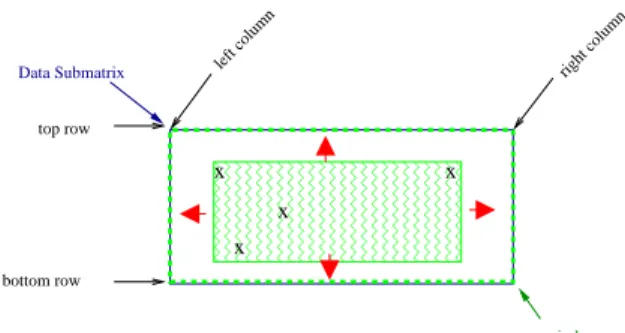
subma-trices and a 2D layout of data is necessary to improve performance. Figure 2 shows a dense window within a data submatrix.
left column
Data Submatrix
top row
bottom row
right column
✁
✁ ✂✁✂
✂✁✂
window ✄☎✄☎✄☎✄☎✄☎✄☎✄☎✄ ✄☎✄☎✄☎✄☎✄☎✄☎✄☎✄ ✄☎✄☎✄☎✄☎✄☎✄☎✄☎✄ ✄☎✄☎✄☎✄☎✄☎✄☎✄☎✄ ✄☎✄☎✄☎✄☎✄☎✄☎✄☎✄
✆☎✆☎✆☎✆☎✆☎✆☎✆☎✆ ✆☎✆☎✆☎✆☎✆☎✆☎✆☎✆ ✆☎✆☎✆☎✆☎✆☎✆☎✆☎✆ ✆☎✆☎✆☎✆☎✆☎✆☎✆☎✆ ✆☎✆☎✆☎✆☎✆☎✆☎✆☎✆
x x
x
Figure 2: A rectangular data submatrix and a window within it.
We have 4 codes specialized in the multiplication
of two matrices. The operation performed is C =
C −A×Bt. The appropriate routine is chosen at
execution time depending on the windows involved in the operation. Their efficiency is different. These
rou-tines (from more to less efficient) are named: FULL,
which uses the entire matrices; WIN 1DC, that uses
windows along the columns; WIN 1DR, which uses
windows along the rows; andWIN 2D, that uses
win-dows in both dimensions and is the slowest amongst all 4 codes.
In [9] we presentedIntra-Block Amalgamation: we
al-low for zeros outside of windows but within data sub-matrices, i.e. we extend the windows if that means that a faster routine can be used. Figure 3 shows how we can extend a window both row and/or column-wise. In case a window is expanded in both directions, the resulting window matches the whole data subma-trix. This action can reduce the number of times a slow matrix multiplication routine is used.
All our previous work was tested on a machine with a MIPS R10000 processor. In this paper we use a dif-ferent machine which has an Intel Itanium2 processor. A preliminary version of this work appeared in [10].
top row
bottom row
left column right column
Data Submatrix
✝✞✝
✝✞✝ ✟✞✟ ✟✞✟
window ✠✡✠✡✠✡✠✡✠✡✠✡✠✡✠✡✠✡✠✡✠✡✠✡✠✡✠✡✠✡✠✡✠✡✠✡✠✡✠✡✠✡✠✡✠✡✠✡✠
✠✡✠✡✠✡✠✡✠✡✠✡✠✡✠✡✠✡✠✡✠✡✠✡✠✡✠✡✠✡✠✡✠✡✠✡✠✡✠✡✠✡✠✡✠✡✠✡✠ ✠✡✠✡✠✡✠✡✠✡✠✡✠✡✠✡✠✡✠✡✠✡✠✡✠✡✠✡✠✡✠✡✠✡✠✡✠✡✠✡✠✡✠✡✠✡✠✡✠ ✠✡✠✡✠✡✠✡✠✡✠✡✠✡✠✡✠✡✠✡✠✡✠✡✠✡✠✡✠✡✠✡✠✡✠✡✠✡✠✡✠✡✠✡✠✡✠✡✠ ✠✡✠✡✠✡✠✡✠✡✠✡✠✡✠✡✠✡✠✡✠✡✠✡✠✡✠✡✠✡✠✡✠✡✠✡✠✡✠✡✠✡✠✡✠✡✠✡✠ ✠✡✠✡✠✡✠✡✠✡✠✡✠✡✠✡✠✡✠✡✠✡✠✡✠✡✠✡✠✡✠✡✠✡✠✡✠✡✠✡✠✡✠✡✠✡✠✡✠
☛✡☛✡☛✡☛✡☛✡☛✡☛✡☛✡☛✡☛✡☛✡☛✡☛✡☛✡☛✡☛✡☛✡☛✡☛✡☛✡☛✡☛✡☛✡☛ ☛✡☛✡☛✡☛✡☛✡☛✡☛✡☛✡☛✡☛✡☛✡☛✡☛✡☛✡☛✡☛✡☛✡☛✡☛✡☛✡☛✡☛✡☛✡☛ ☛✡☛✡☛✡☛✡☛✡☛✡☛✡☛✡☛✡☛✡☛✡☛✡☛✡☛✡☛✡☛✡☛✡☛✡☛✡☛✡☛✡☛✡☛✡☛ ☛✡☛✡☛✡☛✡☛✡☛✡☛✡☛✡☛✡☛✡☛✡☛✡☛✡☛✡☛✡☛✡☛✡☛✡☛✡☛✡☛✡☛✡☛✡☛ ☛✡☛✡☛✡☛✡☛✡☛✡☛✡☛✡☛✡☛✡☛✡☛✡☛✡☛✡☛✡☛✡☛✡☛✡☛✡☛✡☛✡☛✡☛✡☛ ☛✡☛✡☛✡☛✡☛✡☛✡☛✡☛✡☛✡☛✡☛✡☛✡☛✡☛✡☛✡☛✡☛✡☛✡☛✡☛✡☛✡☛✡☛✡☛
x x
x x
Figure 3: Data submatrix after applying both row and column-wise intra-block amalgamation.
1.3
Matrix characteristics
We have used several test matrices. All of them are sparse matrices corresponding to linear programming problems. QAP matrices come from Netlib [11] while others come from a variety of linear multicommodity network flow generators: A Patient Distribution Sys-tem (PDS) [12], with instances taken from [13]; RM-FGEN [14]; GRIDGEN [15]; TRIPARTITE [16]. Ta-ble 1 shows the characteristics of several matrices ob-tained from such linear programming problems. Ma-trices were ordered with METIS [17] and renumbered by an elimination tree postorder [18].
1.4
Contribution
In this paper we present an extension to our previ-ous work on the optimization of a sparse Hyperma-trix Cholesky factorization. We will first summarize the work we have done to adapt our code to a new platform with an Intel Itanium2 processor. Later, we study the effect of a different ordering of the sparse matrices which is more suitable for application on ma-trices arising from linear programming problems. Fi-nally, we present a way to reduce the data submatrix storage, which allows us to try larger matrix sizes. We will present the performance obtained using four different data submatrix sizes.
2
Porting efficiency to a new platform
In this section we summarize the port of our appli-cation from a machine based on a MIPS R10000 pro-cessor to a platform with an Intel Itanium2 propro-cessor. We address the optimization of the sparse Cholesky factorization based on a hypermatrix structure follow-ing several steps.
Table 1: Matrix characteristics: matrices ordered using METIS
Matrix Dimension NZs NZs in L Density of L MFlops to factor
GRIDGEN1 330430 3162757 130586943 0.002 278891
QAP8 912 14864 193228 0.463 63
QAP12 3192 77784 2091706 0.410 2228
QAP15 6330 192405 8755465 0.436 20454
RMFGEN1 28077 151557 6469394 0.016 6323
TRIPART1 4238 80846 1147857 0.127 511
TRIPART2 19781 400229 5917820 0.030 2926
TRIPART3 38881 973881 17806642 0.023 14058
TRIPART4 56869 2407504 76805463 0.047 187168
pds1 1561 12165 37339 0.030 1
pds10 18612 148038 3384640 0.019 2519
pds20 38726 319041 10739539 0.014 13128
pds30 57193 463732 18216426 0.011 26262
pds40 76771 629851 27672127 0.009 43807
pds50 95936 791087 36321636 0.007 61180
pds60 115312 956906 46377926 0.006 81447
pds70 133326 1100254 54795729 0.006 100023
pds80 149558 1216223 64148298 0.005 125002
pds90 164944 1320298 70140993 0.005 138765
at compilation time. We use the best compiler at hand to compile several variants of code. Then, we execute them, and select the one providing best performance. This allows us to create efficient routines which work on small matrices of fixed size. These matrices fit in the lowest level cache. In this way we obtain efficient inner kernels which can exploit efficiently the proces-sor resources. The use of small matrices allows for the reduction of the number of zeros stored within data submatrices.
We have used 4×32 as data submatrix dimensions
since these were the ones providing best performance on the R10000. Later in this paper we will present the results obtained with other matrix dimensions. As we mentioned in section 1.2 we use windows within data submatrices since they have proved effective in reducing both the storage of and operation on zero elements.
Afterwards, we experiment with different intra-block
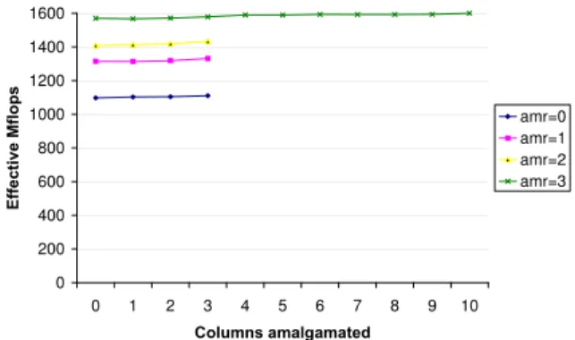
amalgamation values. As an example, figure 4
shows the performance obtained using several val-ues of intra-block amalgamation on the hyperma-trix Cholesky factorization of mahyperma-trix pds20 on an Itanium2. Each curve corresponds to one value of
amalgamation along the rows. The curve at the
top (amr=3) corresponds to the largest amalgama-tion threshold along the rows: three, for submatrices consisting of four rows. The one at the bottom corre-sponds to the case where this type of amalgamation is disabled (amr=0). We must note that we report Effective Mflops. They refer to the number of useful
floating point operations (#flops) performed per sec-ond. Although the time includes the operations per-formed on zeros, this metrics excludes nonproductive operations on zeros performed by the HM Cholesky algorithm when data submatrices contain such zeros. Thus,
Ef f ective M f lops=
#f lops(excluding operations on zeros)·10−6
T ime(including operations on zeros)
On the Itanium2 and using our matrix test suite, the worst performance is obtained when no amalgamation is done along the rows (amr=0). As we allow increas-ing values of the intra-block amalgamation along the rows the overall performance increases. The best per-formance for this matrix dimensions is obtained when amalgamation along the rows is three. This means
that, for data submatrices of size 4×32, we will use no
windows along the rows. This suggests that a larger number of rows could provide improved performance. We will analyze this issue in section 4. As we move right on the curves, we observe the performance ob-tained with increasing values of amalgamation thresh-old along the columns. The difference is often low, but the best results are obtained with values ranging from six to ten.
Figure 4: Sparse HM Cholesky on an Intel Itanium2:
Performance obtained with different values of
intra-block amalgamation on submatrices of size 4×32 on
matrix pds20.
can be different from its aptitudes when dealing with routines which do not use windows at all. And these capabilities can be different from those of the compiler found on another platform. As a consequence we get different optimal values for the intra-block amalgama-tion thresholds on each platform.
3
Sparse matrix reordering
A sparse matrix can be reordered to reduce the amount of fill-in produced during the factorization. Also it can be reordered aiming to improve paral-lelism. In all previous work presented so far we have been using METIS [20] as the reorder algorithm. This algorithm is considered a good algorithm when a par-allel Cholesky factorization has to be done. Also, when matrices are relatively large, graph partitioning algorithms such as METIS usually work much better than MMD, the traditional Minimum Degree order-ing algorithm [21]. METIS implements a Multilevel Nested Dissection algorithm. This sort of algorithms keep a global view of the graph and partition it recur-sively using the Nested Dissection approach [22] split-ting the graph in smaller disconnected graphs. When these subgraphs are considered small, a local ordering algorithm is used. METIS changes to the local order-ing strategy when the number of nodes is less than 200. It uses the MMD algorithm for the local phase.
Although our current implementation is sequential, we have tried to improve the sparse hypermatrix Cholesky for the matrix orders produced by METIS. In this way, the improvements we get are potentially
useful when we go parallel. However, we have also ex-perimented with other classical algorithms. On small matrices in our matrix test suite, when the Multiple Minimum Degree (MMD) [23] algorithm was used the hypermatrix Cholesky factorization took considerably less time. However, as we use larger matrices (RM-FGEN1, pds50, pds60, . . . ) the time taken to factor the resulting matrices became several orders of mag-nitude larger than that of METIS. We have also tried older methods [24] such as the Reverse Cuthill-McKee (RCM) and the Refined Quotient Tree (RQT). RCM tries to keep values in a band as close as possible to the diagonal. RQT tries to obtain a tree partitioning of a graph. These methods produce matrices with denser blocks. However the amount of fill-in is so large that the factorization time gets very large even for medium sized matrices.
3.1
Ordering for Linear Programming
problems
Working with matrices which arise in linear program-ming problems we may use sparse matrix ordering al-gorithms specially targeted for these problems. The METIS sparse matrix ordering package offers some options which the user can specify to change the de-fault ordering parameters. Following the suggestions found in its manual we have experimented with val-ues which can potentially provide improved orderings for sparse matrices coming from linear programming problems. There are eight possible parameters. We skip the details of these parameters for brevity. How-ever, for the sake of completeness, we include the val-ues we have used: 1, 3, 1, 1, 0, 3, 60, and 5.
default configuration. To evaluate the potential for the new ordering parameters we have measured the number of iterations necessary to amortize the cost of the improved matrix reordering. Figure 5 presents the number of iterations after which the specific or-dering starts to be advantageous. We can see that in many cases the benefits are almost immediate. Conse-quently, in the rest of this work we will present results using the modified ordering process specific for matri-ces arising in linear programming problems.
Figure 5: Number of iterations necessary to amortize
cost of improved ordering.
4
Data submatrix size
In section 2 we showed that on an Intel Itanium2
and using data submatrices of size 4 ×32 the
op-timal threshold for amalgamation in the rows was three. This suggests that using data submatrices with a larger number of rows should be tried. However, the larger the blocks, the more likely it is that they con-tain zeros. As we have commented in the introduction and have discussed in previous papers, the presence of zero values within data submatrices causes some drawbacks. Obviously, the computation on such null elements is completely unproductive. However, we al-low them as long as operating on extra elements alal-lows us to do such operations faster. On the other hand, a different aspect is the increase in memory space re-quirements with respect to any storage scheme which keeps only the nonzero values. Next, we present the way in which we can avoid some of this additional storage.
4.1
Data submatrix storage
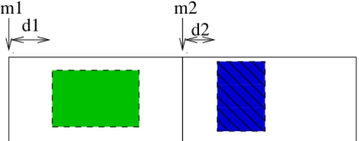
As we mentioned in section 1.2, we use windows to reduce the effect of zeros in the computations. How-ever, we still keep the zeros outside of the window. Figure 6 shows two data submatrices stored contigu-ously. Even when each submatrix has a window we store the whole data submatrix as a dense matrix.
d1
m1
✁ ✁ ✁ ✁ ✁ ✁ ✁ ✁ ✁ ✁ ✁ ✁
m2
d2
Figure 6: Data submatrices before compression.
However, we could avoid storing zeros outside of the window, i.e. just keep the window as a reduced dense matrix. This approach would reduce storage but has a drawback: by the time we need to perform the op-erations we need to either uncompress the data sub-matrix or reckon the adequate indices for a given op-eration. This could have a performance penalty for the numerical factorization. To avoid such overhead we store data submatrices as shown in figure 7.
d1
m1
✂ ✂ ✂ ✂ ✂ ✂ ✂ ✂ ✂ ✂ ✂ ✂
✄ ✄ ✄ ✄ ✄ ✄ ✄ ✄ ✄ ✄ ✄ ✄
m2
d2
Figure 7: Data submatrices after compression.
We do not store zeros in the columns to the left and
right of the window. However, we do keep zeros
above and/or underneath such window. We do this for two reasons: first, to be able to use our routines in the SML which have all leading dimensions fixed at compilation time (we use Fortran, which implies column-wise storage of data submatrices); second, to avoid extra calculations of the row indices. In order to avoid any extra calculations of column indices, we keep pointers to an address which would be the initial address of the data submatrix if we were keeping zero columns on the left part of the data submatrix. Thus, if the distance from the initial address of a submatrix
and its window isdx we keep a pointer to the initial
address of the window with dx subtracted from it.
to the left or right of a window, regardless of having them stored or not.
Figure 8 presents the savings in memory space ob-tained by this method compared to storing the whole
data submatrices of size 4×32. We can observe that
the reduction in memory space is substantial for all matrices.
Figure 8: HM structure: reduction in space after
sub-matrix compression.
4.2
Larger data submatrices:
perfor-mance
The reduction in memory space allows us to experi-ment with larger matrix sizes (except on the largest
matrix in our test suite: GRIDGEN1). Figure 9
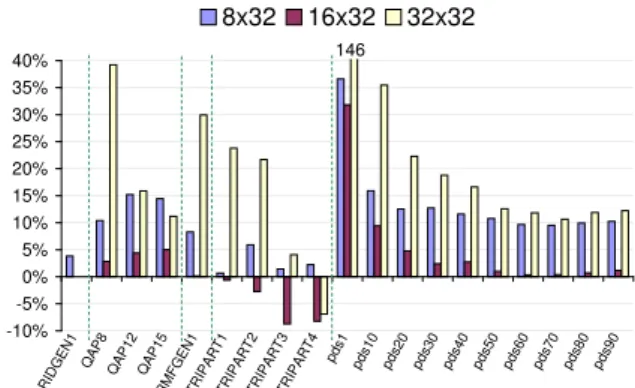
presents the variation in execution time on an Intel Itanium2 processor when the number of rows per data submatrix was increased to 8, 16 and 32. In almost all cases the execution time increased. Only matrices of the TRIPARTITE family benefited from the use of larger submatrices.
Figure 9: Sparse HM Cholesky: variation in execution
time for each submatrix size relative to size 4×32.
We must note that the performance obtained with
matrices of size 8×32 is worse that that obtained
with submatrices of size 16×32. The reason for
this is the relative performance of the routines which work on each matrix size. The one with larger im-pact on the overall performance of the sparse hyper-matrix Cholesky factorization is the one with fixed matrix dimensions and loop trip counts. The cor-responding routine for each matrix size obtains the peak performance shown in table 2. We can observe that the efficiency of the routine working on matrices with four rows is similar to the one which works on matrices with eight rows. However, the overhead, in terms of additional zeros, is much larger for the latter. This explains their relative performance. However, the improved performance of the matrix multiplica-tion routine when matrices have 16 rows can pay off. Similarly to the comparison between codes with eight rows and four, using matrices with 32 rows produces a performance drop with respect to the usage of data submatrices with 16 rows.
Table 2: Performance of theC=C−A×BT
matrix
multiplication routine for each submatrix size.
4×32 8×32 16×32 32×32
4005 4080 4488 4401
5
Conclusions and Future Work
The efficient execution of a program requires the con-figuration of the software to adapt it to the problem being solved and the machine used for finding a solu-tion. We have shown the way in which we can tune our sparse hypermatrix Cholesky factorization code for high performance on a new platform. We have seen that the optimal parameters can be different for each problem type and platform. Thus, we need to adapt the code in search for performance.
We want to improve the performance of our code fur-ther. We believe that some directions for further im-provement can be: modify our sparse hypermatrix Cholesky factorization to have data submatrices ac-cessed with stride one by operating on an upper
trian-gular matrix (U) rather than the lower triangle (L);
of the elimination tree. This will prepare the result-ing hypermatrix for parallel Cholesky factorization, which we plan to implement in the future.
References
[1] Iain S. Duff. Full matrix techniques in sparse Gaussian
elimi-nation. InNumerical analysis (Dundee, 1981), volume 912 of
Lecture Notes in Math., pages 71–84. Springer, Berlin, 1982.
[2] G.Von Fuchs, J.R. Roy, and E. Schrem. Hypermatrix solution
of large sets of symmetric positive-definite linear equations.
Comp. Meth. Appl. Mech. Eng., 1:197–216, 1972.
[3] A. Noor and S. Voigt. Hypermatrix scheme for the STAR–100
computer.Comp. & Struct., 5:287–296, 1975.
[4] M. Ast, R. Fischer, H. Manz, and U. Schulz. PERMAS: User’s
reference manual, INTES publication no. 450, rev.d, 1997.
[5] M. Ast, C. Barrado, J.M. Cela, R. Fischer, O. Laborda,
H. Manz, and U. Schulz. Sparse matrix structure for dynamic
parallelisation efficiency. InEuro-Par 2000,LNCS1900, pages
519–526, September 2000.
[6] Jos´e R. Herrero and Juan J. Navarro. Improving
Perfor-mance of Hypermatrix Cholesky Factorization. In
Euro-Par’03,LNCS2790, pages 461–469. Springer-Verlag, August
2003.
[7] Jos´e R. Herrero and Juan J. Navarro. Reducing overhead
in sparse hypermatrix Cholesky factorization. InIFIP TC5
Workshop on High Performance Computational Science and
Engineering (HPCSE), World Computer Congress, pages
143–154. Springer-Verlag, August 2004.
[8] Jos´e R. Herrero and Juan J. Navarro. Optimization of a
statically partitioned hypermatrix sparse Cholesky
factoriza-tion. InWorkshop on state-of-the-art in scientific computing
(PARA’04),LNCS3732, pages 798–807. Springer-Verlag, June
2004.
[9] Jos´e R. Herrero and Juan J. Navarro. Intra-block
amalga-mation in sparse hypermatrix Cholesky factorization. InInt.
Conf. on Computational Science and Engineering, pages 15–
22, June 2005.
[10] Jos´e R. Herrero and Juan J. Navarro. Sparse hypermatrix
Cholesky: Customization for high performance. In
Proceed-ings of The International MultiConference of Engineers and
Computer Scientists 2006, June 2006.
[11] NetLib. Linear programming problems.
[12] W.J. Carolan, J.E. Hill, J.L. Kennington, S. Niemi, and S.J.
Wichmann. An empirical evaluation of the KORBX
algo-rithms for military airlift applications. Oper. Res., 38:240–
248, 1990.
[13] A. Frangioni. Multicommodity Min Cost Flow problems.
Op-erations Research Group, Department of Computer Science,
University of Pisa.
[14] Tamas Badics. RMFGEN generator., 1991.
[15] Y. Lee and J. Orlin. GRIDGEN generator., 1991.
[16] Andrew V. Goldberg, Jeffrey D. Oldham, Serge Plotkin, and
Cliff Stein. An implementation of a combinatorial
approxi-mation algorithm for minimum-cost multicommodity flow. In
Proceedings of the 6th International Conference on Integer
Programming and Combinatorial Optimization, IPCO’98
(Houston, Texas, June 22-24, 1998), volume 1412 ofLNCS,
pages 338–352. Springer-Verlag, 1998.
[17] George Karypis and Vipin Kumar. A fast and high quality
multilevel scheme for partitioning irregular graphs. Technical
Report TR95-035, Department of Computer Science,
Univer-sity of Minnesota, October 1995.
[18] J. W. Liu, E. G. Ng, and B. W. Peyton. On finding supernodes
for sparse matrix computations.SIAM J. Matrix Anal. Appl.,
14(1):242–252, January 1993.
[19] Jos´e R. Herrero and Juan J. Navarro. Automatic
benchmark-ing and optimization of codes: an experience with numerical
kernels. InInt. Conf. on Software Engineering Research and
Practice, pages 701–706. CSREA Press, June 2003.
[20] George Karypis and Vipin Kumar. METIS: A Software
Package for Partitioning Unstructured Graphs, Partitioning
Meshes, and Computing Fill-Reducing Orderings of Sparse
Matrices, Version 4.0, September 1998.
[21] Nicholas I. M. Gould, Yifan Hu, and Jennifer A. Scott. A
numerical evaluation of sparse direct solvers for the solution of
large sparse, symmetric linear systems of equations. Technical
Report RAL-TR-2005-005, Rutherford Appleton Laboratory,
Oxfordshire OX11 0QX, April 2005.
[22] Alan George. Nested disection of a regular finite element mesh.
SIAM Journal on Numerical Analysis, 10:345–363,
Septem-ber 1973.
[23] J. W. H. Liu. Modification of the minimum degree algorithm
by multiple elimination.ACM Transactions on Mathematical
Software, 11(2):141–153, 1985.
[24] A. George and J. W. H. Liu. Computer Solution of Large
Sparse Positive-Definite Systems. Prentice-Hall, Englewood