Integrated response and transit time distributions of watersheds by combining hydrograph separation and long-term transit time modeling

(1)

HESSD

7, 1–32, 2010

Response and transit time distributions of

watersheds

M. C. Roa-Garc´ı_{a and} M. Weiler

Title Page

Abstract Introduction

Conclusions References

Tables Figures

◭ ◮

Back Close

Full Screen / Esc

Printer-friendly Version

Interactive Discussion Hydrol. Earth Syst. Sci. Discuss., 7, 1–32, 2010

www.hydrol-earth-syst-sci-discuss.net/7/1/2010/ © Author(s) 2010. This work is distributed under the Creative Commons Attribution 3.0 License.

Hydrology and Earth System Sciences Discussions

This discussion paper is/has been under review for the journal Hydrology and Earth System Sciences (HESS). Please refer to the corresponding final paper in HESS if available.

Integrated response and transit time

distributions of watersheds by combining

hydrograph separation and long-term

transit time modeling

M. C. Roa-Garc´ıa1,2and M. Weiler3

1

Land and Food Systems, University of British Columbia, 2357 Main Mall, Vancouver, BC, V6T 1Z4, Canada

2

Fundaci ´on Evaristo Garc´ıa, AA 4443 Cali, Colombia

3

Institute of Hydrology, University of Freiburg, Fahnenbergplatz, 79098 Freiburg, Germany Received: 6 December 2009 – Accepted: 13 December 2009 – Published: 6 January 2010 Correspondence to: M. C. Roa-Garc´ıa ([email protected])

Published by Copernicus Publications on behalf of the European Geosciences Union.

(2)

HESSD

7, 1–32, 2010

watersheds

Title Page

Tables Figures

◭ ◮

Back Close

Full Screen / Esc

Interactive Discussion

Abstract

We present a new modeling approach analyzing and predicting the Transit Time Dis-tribution (TTD) and the Response Time DisDis-tribution (RTD) from hourly to annual time scales as two distinct hydrological processes. The model integrates Isotope Hydro-graph Separation (IHS) and the Instantaneous Unit HydroHydro-graph (IUH) approach as a

5

tool to provide a more realistic description of transit and response time of water in catchments. Individual event simulations and parameterizations were combined with long-term baseflow simulation and parameterizations to provide a comprehensive pic-ture of the catchment response for a long time span for the hydraulic and isotopic processes. The proposed method was tested in three Andean headwater catchments

10

to compare the eff_{ects of land use on hydrological response and solute transport.} Re-sults show that the characteristics of events and antecedent conditions have a signif-icant influence on TTD and RTD, but in general the RTD of the grassland dominated catchment is concentrated in the shorter time spans and has a higher cumulative TTD, while the forest dominated catchment has a relatively longer response distribution and

15

lower cumulative TTD. The catchment where wetlands concentrate shows a flashier response, but wetlands also appear to contribute to prolong transit time.

1 Introduction

Water management whose aim is to sustain catchment ecological services requires an understanding of the hydrologic cycle. Comparative analysis of catchment

behav-20

ior allows observing the eff_{ects of human activities on the amount and rate of water} flows, the eff_{ects of land use change on water quantity and quality, the persistence} of soluble contaminants in catchments, and the vulnerability of ecosystems to be im-pacted by climate change. Comparing flows, residence time and transit time of water from catchments with similar size, topography and soil type, enables us to understand

25

(3)

HESSD

7, 1–32, 2010

watersheds

Title Page

Tables Figures

◭ ◮

Back Close

Full Screen / Esc

Interactive Discussion Stable water isotopes have been used in hydrology for two purposes: 1) to identify

the temporal variations of water contribution for baseflow and for individual storms; and 2) to identify the source of runoff_{during an event, e.g. whether it comes from rain} or snowmelt (event water) or from water stored in the watershed prior to the event (groundwater, soil water, lakes etc.) (Vitvar et al., 2005). This knowledge has been

5

used to understand the interactions between precipitation, runoff_{pathways and runo}ff generation processes, and as a proxy for the capacity of a catchment to store water and chemicals and regulate its flow.

The models used to analyze isotope data in hydrology have been developed on ear-lier hydrological tools focused on graphical separations of stream flow components

10

(e.g. quick and slow flows) and unit hydrograph models to predict peak discharge and to extract lumped physical characteristics of drainage basins (Sherman, 1932; Clark, 1945; Barnes, 1940; Hewlett and Hibbert, 1967). Later, tracers have been used in a more objective way to separate the storm hydrograph. Stable isotope hydrograph separations (IHS) (Pinder and Jones, 1969; Sklash et al., 1976) and conservative

geo-15

chemical tracing (Hooper and Shoemaker, 1986) have been developed into common tools in watershed hydrology (Kendall and Caldwell, 1998). These tracer-based sep-aration approaches have the advantage of providing more process-based information about temporal and geographic sources of runoff_.

Lumped transport models to estimate the transit time of water in catchments or other

20

hydrological systems (groundwater, unsaturated zone) have been developed in parallel to predict the transit time distribution (TTD) and mean transit time (MTT) of a system (Maloszewski and Zuber, 1982). These models have been used mostly under baseflow conditions in catchments since an important assumption is stationarity of runoff_{. A} detailed review of the diff_{erent models, applications and assumptions can be found in}

25

McGuire and McDonnell (2006).

Other approaches to simulate and analyze TTD include one developed by Kirchner et al. (2001), which combined diff_{erent transport models (advection-dispersion,} expo-nential and gamma models) and the observed fractal scaling in rainfall and catchment

(4)

HESSD

7, 1–32, 2010

watersheds

Title Page

Tables Figures

◭ ◮

Back Close

Full Screen / Esc

Interactive Discussion runoff_{and chemistry in the spectral domain. This approach implies a large number}

of parameters that are not possible to test in models that are not disaggregated into individually parameterized compartments (Kirchner et al., 2001). Botter et al. (2005) discussed stochastic models that embed spatial variability and uncertainty into a math-ematical framework of a reduced number of parameters. They evaluated models

in-5

cluding the mass response functions which they suggest as an appropriate generic transport model for catchments. More recently Botter et al. (2010) have explored non-linearities in travel time distributions associated with time-varying rainfall, runoff _and evapotranspiration processes, proposing a transport model that considers catchments as nonlinear systems with memory (Botter et al., 2010).

10

Despite the common use of IHS and transit time modeling in hydrology, the combi-nation and integration of the two approaches has not yet been explored. Our approach builds upon the work of McDonnell et al. (1999) and Weiler et al. (1999), whereby the temporal variability in rainfall isotopic composition during an rainfall event is used to model event based transit time distribution (analogous to the annual time series

ap-15

proach of Maloszewski and Zuber, 1982) and to compute event and pre-event water contributions to storm runoff_{. We thus estimate event water transit time distributions} for discrete events (building upon Unnikrishna et al., 1995). In eff_{ect, their work was} an attempt to combine the process merits of tracer-based hydrograph separation with the hydraulic transfer function approach of the unit hydrograph in an eff_{ort to increase}

20

the information gained from the storm hydrograph. This new method of hydrograph separation embraces the temporal variability of rainfall isotopic composition, but in-cludes a new transfer function for event water and pre-event water determined from the time-variable event water fraction. A transfer function representing the runoff_response (i.e. the instantaneous unit hydrograph) is used to constrain the event residence time

25

(5)

HESSD

7, 1–32, 2010

watersheds

Title Page

Tables Figures

◭ ◮

Back Close

Full Screen / Esc

Interactive Discussion this paper that both responses are essential to understand catchment behavior, since

one response (i.e. the transit time) represents actual conservative solute travel time (i.e. along flowpaths) and the other represents hydraulic dynamics (e.g. rainfall-runoff response).

We present a new methodology that combines the isotope hydrograph separation

5

and long term transit time modeling to provide realistic information about the response and transit time of water in catchments over several orders of temporal scales. We use this model to compare the eff_{ect of land use on the hydrological response of three} small headwater catchments in the mountains of Colombia, that constitute the water source for a municipality of 15 000 people and their economic activities.

10

2 Methods

2.1 Study site and dataset

Three adjacent small headwater catchments draining to the same river system were selected for a comparative study of land use and stream flow to quantify the impact that diff_{erent land use types have on stream flow. These catchments are located in the}

15

coff_{ee growing region of Colombia (Fig. 1), on the western side of the central branch of} the Andes and drain to the Cauca River, which flows north to the Atlantic Ocean. Most of the land in the three micro-catchments is dedicated to extensive cattle rearing but diff_{erences in land use can be seen among the three catchments. The parent materials} of the soil are fluvio-volcanic sediments (mostly clays of uniform size and arranged with

20

pockets of crystalline coarse fragments). The geological unit has a volcanic ash layer which can reach up to tens of meters in thickness at some locations, is characterized by very low hydraulic conductivity, which contributes to the formation of wetlands, limits water percolation and contributes to maintaining a high water table. Soils formed on these sediments are classified as Andisols (Acrudoxic Hapludans) (IGAC, 1996)

char-25

acterized by high organic matter content and high content of allophanes and imogolite, which combined produce soils of high water holding capacity.

(6)

HESSD

7, 1–32, 2010

watersheds

Title Page

Tables Figures

◭ ◮

Back Close

Full Screen / Esc

Interactive Discussion The catchments (B1, B2 and BB) diff_{er in size and land use (Table 1). BB is the}

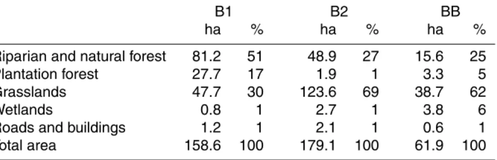
smallest catchment, but has the largest proportion of wetlands. B2 is the largest catch-ment with the highest proportion of grasslands. And B1 is smaller than B2 but has a larger proportion of natural and riparian forest.

Streamflow was monitored at the outlet of the three catchments. Water level was

5

recorded every 15 min from June 2005 until May 2007 with three AquiStar PT2X Smart Sensors© at the catchment outlet. The water level data series were converted into discharge measurements with stage-discharge relations using 62, 44 and 50 discharge measurements for catchments B1, B2 and BB respectively measuring discharge using a current meter from OTT. Precipitation was measured using three Hobo Pro data

10

logging rain gauges located in each catchment.

Rain samples were taken every two weeks from November 2005 until May 2007 (n=_{39). Rain was collected according to guidelines from the isotope hydrology} labora-tory of the International Atomic Energy Agency – IAEA (2002). The water accumulated every two weeks was mixed in the container and a sample was taken at the end of the

15

sampling period. At all stream gauging stations, stream water samples were manually taken every two weeks, from May 2006 to May 2007 (n=_332).

Seven storm events were sampled during two rainy seasons in 2006 and 2007, of which five events were selected for modeling due to their completeness: 14 Novem-ber 2006 (event 2), 21 NovemNovem-ber 2006 (event 3), 7 April 2007 (event 5), 18 April 2007

20

(event 6) and 25 April 2007 (event 7). The rain samples were taken manually and a group of six people participated in the collection of samples for each event. The se-quence of rain samples was determined by the speed at which vials could be filled with rain. From the three streams a baseflow sample was taken before the rain started. Once the water level started rising, samples were taken every 20 min until the peak was

25

(7)

HESSD

7, 1–32, 2010

watersheds

Title Page

Tables Figures

◭ ◮

Back Close

Full Screen / Esc

Interactive Discussion expected in the first few hours of the afternoon. If chances of a storm were relatively

high one person was stationed in each catchment outflow from the beginning of the storm until the last sample of the 30 min intervals was taken; after that, a group of three people would move between the sites to collect the samples every two hours. The number of samples was 104 for event 2, 83 for event 3, 71 for event 5, 95 for event

5

6, and 86 for event 7. Precipitation and discharge samples were taken in high den-sity polyethylene scintillation vials with cone caps. The oxygen isotopic composition of samples was determined at the mass spectroscopy laboratory of the University of Idaho. Theδ18O values are reported in per mil (‰) relative to the standard (VSMOW) with an analytical error of±0.08 ‰.

10

2.2 Estimating RTD and TTD for events and baseflow conditions

The integrative models applied at the two time scales (the short-term, event and the long-term, baseflow scales) estimate the response time distribution (RTD) and the tran-sit time distribution (TTD). These responses are typically decoupled with the displace-ment of stored water during rainfall periods and the slow drainage during dry

peri-15

ods and the rapid response of new water inputs via well-connected pathways (Bonell, 1998). The Mean Transit Time (MTT) is defined as the average time elapsed since water drops entered the catchment and the time they are observed in the catchment outlet (Vitvar et al., 2005). Mean Response Time (MRT) on the other hand, is an indi-cator of the rainfall-runoff_{response as it represents the speed and volume of outflow}

20

with which a catchment responds to water input (precipitation). Since the fluctuations in hydraulic head (the driving force in water flux) can propagate much faster than in-dividual water molecules, the MRT is expected to be shorter than the MTT. The TTD describes the distribution of times that each molecule of water takes to arrive at the catchment outlet from all locations in the catchment (McGuire and McDonnell, 2006).

25

The response time distribution or RTD is the integrated response time of a catchment to a unit rainfall input and is similar to the unit hydrograph concept.

(8)

HESSD

7, 1–32, 2010

watersheds

Title Page

Tables Figures

◭ ◮

Back Close

Full Screen / Esc

Interactive Discussion The models to estimate RTD and TTD for individual events and under baseflow

condition were further developed from the TRANSEP model, which is a quantitative approach to describe the transit time and transmittance of hydraulic behavior to help understand the relationship between pre-event and event water delivery to streams (Weiler et al., 2003). It uses water flux and isotopic data from precipitation and

stream-5

flow to derive transfer functions of runoff_{, event and pre-event water by capitalizing} on the temporal variation of rainfall tracer composition. The transfer function can be chosen from transfer functions previously designed including the exponential distribu-tion, the exponential piston-flow distribution and the advection-dispersion model (Mal-oszewski and Zuber, 1982), the gamma distribution (Kirchner, et al., 2001), or the two

10

parallel linear reservoirs model (Weiler et al., 2003). Weiler et al. (2003) tested these models and obtained best results from the two parallel linear reservoirs (TPLR). Other studies (Hrachowitz et al., 2009; McGuire et al., 2005) also showed that the TPLR model produces good results. The TPLR was the transfer distribution used for the present study.

15

The input data for event analysis with this model corresponds to precipitation inten-sity and streamflow in 15 min intervals and the corresponding isotope composition for precipitation in those time intervals for the duration of the precipitation event sampled for approximately 24 hours. The input data for the baseflow analysis with the model cor-responds to precipitation and streamflow in daily intervals and using bi-weekly isotope

20

composition records for 12 months in the streams (May 2006 to May 2007), bi-weekly precipitation isotope composition records for 19 months (November 2005 to May 2007), and precipitation records of 29 months (January 2005 to May 2007). When the MTT in a catchment is suffi_{ciently longer than the input record, parameters such as MTT will be} poorly estimated. With a MTT of around one year, only a record of five years or longer

25

(9)

HESSD

7, 1–32, 2010

watersheds

Title Page

Tables Figures

◭ ◮

Back Close

Full Screen / Esc

Interactive Discussion The models to estimate RTD for the short and long time scale are both simple

rainfall-runoff_{model that simulates streamflow by a non-linear and a linear module, similar to} a variety of instantaneous unit hydrograph (IUH) based models (Bras, 1990). The non-linear module is the loss function generating an eff_{ective precipitation time series} (Jakeman and Hornberger, 1993):

5

s(t)=_b₁_p₍_t₎+₁₋_b−1 2

s(t−∆t) (1)

peff(t)=p(t)s(t) (2)

wherepeff(t) is the effective precipitation,s(t) is the antecedent precipitation index that

is calculated by exponentially weighting the precipitation backward in time according to the parameter b2. The parameter b1maintains the water balance over the simulation

10

period and thus can be determined directly from the rainfall- runoff _{data. The runo}ff coeffi_{cient rc for each temporal scale can be defined as the total e}ff_{ective precipitation} divided by the total precipitation. The runoff_coeffi_{cients for the events are a reflection} of runoff _{generation processes and storage; for the longer time scale, the di}ff_erence between precipitation and eff_{ective precipitation is due to evapotranspiration. The}

lin-15

ear module describes a convolution of the eff_{ective precipitation and runo}ff _transfer function:

Q(t)= Zt

0

g(τ)peff(t−τ)d τ (3)

whereg(τ) is the response time distribution (RTD), defined for the long term (b) and event (e) scale, and thus the rainfall-induced response of catchment runoff_.

20

To estimate the streamflow concentration C(t) for the baseflow model we use the tracer mass flux instead of the tracer concentration since the tracer signal depends on the actual tracer mass flux, which depends on the eff_{ective precipitation (Stewart and} McDonnell, 1991; Weiler et al., 1999):

C(t)= Rt

0Cin(t−τ)peff(t−τ)h_b(τ)d τ

Rt

0peff(t−τ)hb(τ)d τ

(4)

25

(10)

HESSD

7, 1–32, 2010

watersheds

M. C. Roa-Garc´ı_{a and} M. Weiler Title Page Abstract Introduction Conclusions References Tables Figures ◭ ◮ ◭ ◮ Back Close

Full Screen / Esc

Interactive Discussion wherehb(τ) is the long-term transit time distribution andCin is the observed input

con-centration in the precipitation. As introduced into the TRANSEP model, the event water transit time distributionhe(τ) can be calculated in a similar way by focusing on individual

events and including the eff_{ect of event and pre-event water runo}ff_{during the events.} The concentrationC(t) in the stream is then given by (Weiler et al., 2003):

5

C(t)= Rt

0Cin(t−τ)peff(t−τ)f(t−τ)he(τ)d τ

Rt

0peff(t−τ)f(t−τ)he(τ)d τ

(5)

The main diff_{erence to Eq. (4) is}_f_{, the fraction of e}ff_{ective precipitation that becomes} event water (i.e. “new” water), and he(τ) is the transfer function of the event water

(i.e. the transit time distribution). The denominator of Eq. (5) is equal to the event water runoff_{(Weiler et al., 2003) and the total event water fraction}_F _{can then be derived.}

10

As already discussed we use the two parallel linear reservoirs as our transfer function for the RTD and TTD and for both time scales:

g(τ)=_h_b₍_τ₎=_h_e₍_τ₎=φ τf exp −τ τf

+1−φ τs exp −τ τs (6)

Whereτ_f and τ_s are the mean response times of the fast and slow responding reser-voirs, respectively. The parameter φ defines the partition of the input into the fast

15

responding reservoir.

We used ant colony optimization to the inverse estimation problem of the unknown parameters (Abbaspour et al., 2001) for both time scales. It has been shown that this technique effi_{ciently finds the optimum solution for a wide range of applications. First,} the parameter of the response time model was optimized using precipitation as input

20

(11)

HESSD

7, 1–32, 2010

watersheds

Title Page

Tables Figures

◭ ◮

Back Close

Full Screen / Esc

2.3 Combining RTD and TTD from events and baseflow modeling

The estimated RTD and TTD for the two time scales (minutes for the events and days for the baseflow) are describing a hydrological system (i.e. watershed) with diff_erent temporal resolution. In order to derive a RTD or TTD distribution that describes a catchment from minutes to years, we can combine the two distributions for the events

5

and the baseflow. To do this, we select the distribution from an individual event and combine it with the overall distribution from the baseflow analysis. This can be done for diff_{erent events and the RTD or TTD will show the time variant behavior of the} catchment according to the event characteristics. This is similar to the observations made by McGuire et al. (2007). The combined RTDg(τ) and TTD h(τ) is then given

10

by:

g(τ)=_rc_e_g_e₍_τ₎+₍₁₋_rc_e₎_g_b₍_τ₎ ₍₇₎

h(τ)=

rc_eF h_e(τ)+₍₁₋_rc_e_F₎_h_b₍_τ₎

rc_b (8)

The integral of the RTD will be unity, but as can be seen in Eq. (8), the integral of the TTD can be less than unity. The idea behind this new concept is that for an open

sys-15

tem like a catchment, part of the water molecules entering the system as precipitation will leave the catchment not through the stream but by evapotranspiration. Hence, a TTD can in a strict way not approach unity for most catchments as part of the water molecules that entered the system during a precipitation event never reach the stream. This idea is similar to the stochastic concept of an evapotranspiration time probability

20

distribution function pdf proposed by Botter et al. (2010).

(12)

HESSD

7, 1–32, 2010

watersheds

Title Page

Tables Figures

◭ ◮

Back Close

Full Screen / Esc

3 Results

3.1 RTD and TTD of rainfall-runo_ffevents

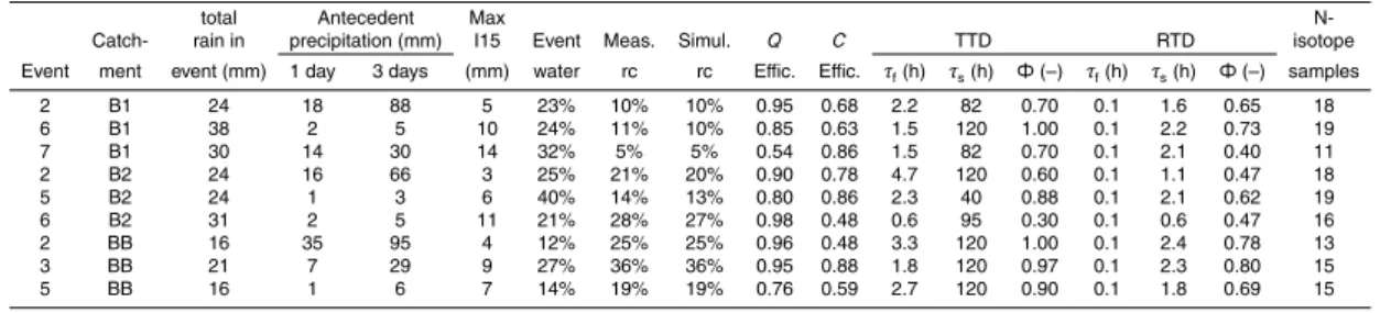
For this analysis an event is defined as precipitation equal or larger than 2 mm that ends when there has been no precipitation for the following 2 h. Five sampled storms were analyzed using TRANSEP for the three catchments. The results are shown in

5

Table 2. Results include event water, defined as the proportion of stream discharge during an event that originates from precipitation (Buttle, 1994) and runoff_coeffi_cient which corresponds to the proportion of rainfall that becomes stream discharge during an event. For each of the two processes (transit of individual water molecules and the response of catchments) three parameters are optimized: the transit/response time of

10

the fast reservoir (τf), the transit/response time of the slow reservoir (τs) and the portion

of the total discharge corresponding to the fast reservoir (Φ_{) for individual events.} The model was generally able to predict the observed runoff_{response as the} Nash-Suttcliff_Effi_{ciency is larger than 0.8 for almost all events. The prediction of the isotopes} variation in the streamflow with TRANSEP was also acceptable. Generally, the RTD is

15

dominated by the fast reservoir with a very rapid response time below 1 h. The TTD is more delayed, but dominated by the fast reservoir. For a couple of events, the two linear reservoirs are simplified to an exponential model since the portion of the total discharge corresponding to the fast reservoir is equal to unity.

There is not a large diff_{erence in pre-event water between B1 (forest dominated}

20

catchment) and B2 (grassland dominated catchment). Catchment BB however, seems to produce larger pre-event water, which could be linked to the presence of wetlands in 6% of the catchment area. Catchments B2 and BB are relatively similar in their runoff coeffi_{cients while B1’s seem significantly lower. Catchments B2 and BB have similar} distribution of land coverage, with grasslands as the dominant land use (69% and 62%

25

(13)

HESSD

7, 1–32, 2010

watersheds

Title Page

Tables Figures

◭ ◮

Back Close

Full Screen / Esc

Interactive Discussion Antecedent precipitation combined with the size of the event, are major factors in

determining the percentage of pre-event water in the total discharge. For this reason it is reasonable to compare the events for similar antecedent precipitation conditions. Event 2 is a good illustration of the diff_{erences between catchments B1 and B2 since} antecedent precipitation conditions and the characteristics of the event were similar

5

for the two catchments. BB’s antecedent precipitation for 1 day was higher than for the other two catchments which might explain the large volume of catchment BB’s response and the high pre-event water contribution (88%), despite a smaller event (16 mm compared with 24 mm in the other two catchments). However, the eff_{ect of a} 6% of area in wetlands should not be discarded as a source of pre-event water.

10

3.2 RTD and TTD of baseflow

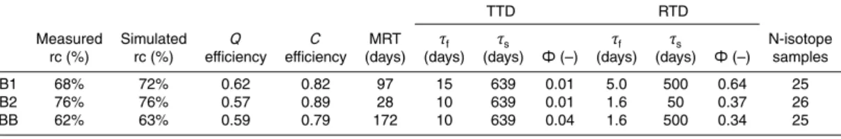
Results of the Transit Time model for the baseflow samples taken every two weeks are shown in Table 3. The three catchments have relatively high yields. Runoff_coeffi_{cient –} rc is defined as the proportion of rainfall that becomes stream discharge on an annual basis. B2, with a rc of 76% is the catchment with the smallest infiltration and storage

15

capacity when it rains, and thus a larger proportion of rainfall becomes runoff_{. BB,} despite having a similar percentage of forest cover than B2, has the lowest rc, point-ing to the higher proportion of wetland area that would contribute to store water and preventing a higher proportion of runoff_.

The mean response times indicate that the water that enters B2 catchment takes

20

28 days to reach the catchment outflow, being the catchment with the shortest mean response time; the water that enters B1 takes 97 days to leave the catchment and for BB catchment, the water takes 172 days to leave. The wetlands in BB could be the main explanation for the longer mean response time of water in BB; and the forests in B1 could explain the intermediate response time of water for this catchment. The

25

separation of the input water into the slow and the fast compartments shows that it is the mean response time of the slow reservoir that is significantly shorter for B2 than for

(14)

HESSD

7, 1–32, 2010

watersheds

Title Page

Tables Figures

◭ ◮

Back Close

Full Screen / Esc

Interactive Discussion the other two catchments (50 days versus 500 days), which draws down the total mean

response time for B2. Catchment B2, despite a relatively large slow reservoir portion, has a short MRT due to its short MRT for the slow reservoir.

3.3 Comparing integrated RTD and TTD

The integration of event and baseflow data to generate RTD and TTD allows a

com-5

parison of catchments on a long time scale by incorporating the influence of individual events. Figure 2 compares the response of the three studied catchments for event 2, which was a relatively large event in catchments B1 and B2 where antecedent precip-itation was low and a medium size event for catchment BB (Table 2). The resulting RTD curves which illustrate the hydrological response of the catchments show a

sig-10

nificantly shorter RTD for catchment B2. This is influenced by the land use diff_erences between the three catchments, since B2 is the catchment dominated by grasslands with a more limited water storage capacity than the catchments dominated by forest or with a significant portion of wetlands. Additionally the curves show the eff_{ect that} antecedent precipitation conditions have on RTD at the short time scale. The curve for

15

BB shows a faster response in the first half day after the event. The cumulative linear curves clearly show that the response from BB was faster during the first few days after the event. These curves also show that B1, the forest dominated catchment, had the slowest response and hence the largest overall storage.

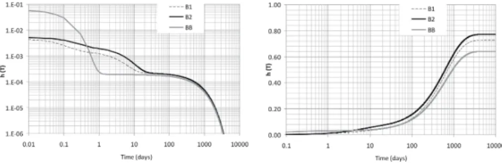
Diff_{erences between the TTD of the three catchments can be seen in the probability}

20

and cumulative distribution function of the TDD as shown in Fig. 3. The large diff er-ences observed between the three catchments for the short times are determined by the runoff _coeffi_{cients of the di}ff_{erent events, which in turn respond to the influence} of the size and intensity of the event and the antecedent precipitation conditions in each of the catchments. The cumulative TTD in the longer time scale show the

in-25

(15)

HESSD

7, 1–32, 2010

watersheds

Title Page

Tables Figures

◭ ◮

Back Close

Full Screen / Esc

Interactive Discussion looses more water in the longer time range through evapotranspiration, followed by the

catchment dominated by forests (B1). Also the catchment with the highest proportion of wetlands (BB) has the highest proportion of water leaving the watershed within the first day.

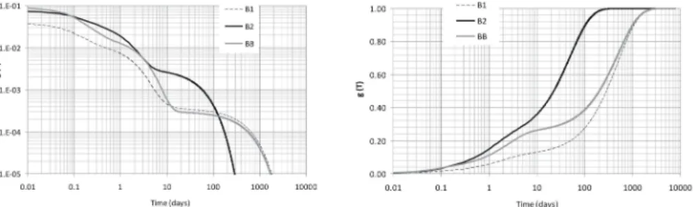
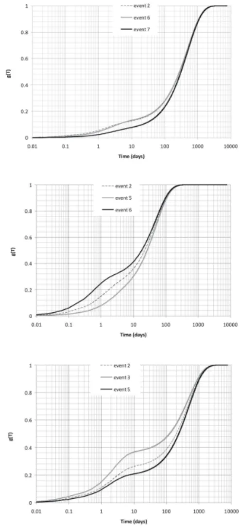
The comparison of RDT for the three catchments for diff_{erent events, shown in Fig. 4,}

5

illustrate similarities between catchments B2 and BB in terms of the pdf at short times (revolving around 0.1) in contrast to the pdf of B1 with values below around 0.01. These pdfs highlight the impact of forests (B1) on water holding capacity and the dampening of storm flows. For the larger times, a diff_{erence can be seen between B2 (the} grass-land catchment) and the other two catchments that show a higher frequency of longer

10

response suggesting the influence of forests and wetlands as a long term water stor-age. This can also be seen in the cumulative RTD as B2 is close to reaching unity after 100 days, but takes over 1000 days for the other two catchments. The cumula-tive curves show significant diff_{erences between the three catchments. The curves for} three diff_{erent events for catchment B1 are flatter and have less dispersion than the}

15

same curves for the other two catchments. This gives the idea that this catchment has a slower response likely as a result of the higher percentage of forest coverage. B2 and BB appear to have a more variable response, but B2 shows a noticeably faster response, which can be seen around the 10 days mark at which a larger proportion of water has left catchment B2 indicating a reduced capacity to store water related to

be-20

ing predominantly grassland. Generally, the RTD are most variable up to 10 days due to the non-linear response of runoff_{to rainfall as a function of rainfall characteristics} and antecedent conditions.

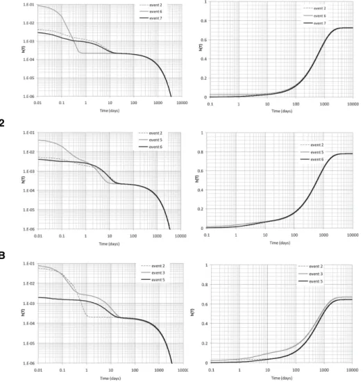
The comparison of the TTD for the individual catchments in Fig. 5 shows a simi-lar picture as for the RDT, but with much less variability between events within one

25

catchment. The variability of cumulative event water contribution among rainfall events is much smaller than the variability of runoff _{response and runo}ff _coeffi_{cients among} events. In the right column of Fig. 5 it is shown that the proportion of water leaving the watershed within the first 10 days is very similar for most events and below 10%

(16)

HESSD

7, 1–32, 2010

watersheds

Title Page

Tables Figures

◭ ◮

Back Close

Full Screen / Esc

Interactive Discussion for all watersheds, but smaller for B1. It is also apparent that BB looses more water to

evapotranspiration, as the cumulative TTD in the longer time scale is smaller than for the other two catchments.

4 Discussion

4.1 A new response time and transit time distribution

5

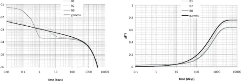
According to a transit time study conducted with the use of chloride as a tracer for the Plynlimon catchments near the coast of Wales (Kirchner et al., 2001), the gamma distribution is an empirically adequate description of the attenuation of chloride con-centration from the rainfall to the streamflow. This distribution has also proven to be a robust description of the transit time in many other catchments (Kirchner et al., 2001;

10

Hrachowitz et al., 2009). A gamma distribution is fitted to the observed TTD for event 2 of the three watersheds in Fig. 6 using the runoff _coeffi_{cient to reduce the integral} of unity to 0.74. The two parameters of the gamma distribution, α and β were esti-mated as 0.7 and 800, resulting in a MTD of 560 days. The range of α between 0.5 and 1.0 is in accordance to the observations made in other watersheds. However, the

15

gamma distribution does not adequately describe the short term behavior of the TTD in most cases. This implies that the movement of water in short time spans (less than 10 days) is significantly influenced by individual precipitation events and the dynamics of rainfall-runoff_{response processes as also shown by McGuire et al. (2007). The method} implies that TTD of catchments are not necessarily represented through gamma

dis-20

tributions as has been suggested earlier (Kichner et al., 2001). It also highlights the issue of applying a steady-state model to catchments over diff_{erent time scales. In} ad-dition, the resolution of sampling could influence the results in particular for the shorter time scales. The integration of event TTD with a high resolution of sampling of isotope composition for individual events allows seeing diff_{erences in catchment responses at}

25

(17)

HESSD

7, 1–32, 2010

watersheds

Title Page

Tables Figures

◭ ◮

Back Close

Full Screen / Esc

Interactive Discussion (events) with lower frequency sampling (baseflow) is possible with the process-based

approach presented here but has to be applied carefully when using spectral analysis (Feng et al., 2004).

The integration of the two time scales is proposed here as a new tool to compare catchments. Although only individual events can be incorporated into the approach,

5

the resulting RTD and TTD provide a comprehensive image of the catchment response over a long time range for the hydraulic and isotopic processes. The proposed method allowed a comparison between catchments for several events and showed that incor-porating individual events into a longer time frame provides a comprehensive view of water movement in catchments.

10

Comparisons at diff_{erent time scales have been done for several years. Hydrograph} separation of events using TRANSEP illustrated the diff_{erences that land use has on} water flow regulation and the source of water during storm events. Two main findings arise from this comparison: 1) the grassland dominated catchment B2 has a higher event response in relation to the forest dominated catchment B1, but both of them show

15

a similar composition of event and pre-event water; and 2) even a small percentage of area in wetlands (6% of catchment area for BB) drain a high percentage of old water during storm events related to the higher connectivity of saturated areas to the dis-charge network. These findings coincide with what has been found in previous studies both in temperate environments (Genereux and Hooper, 1998) and in tropical

environ-20

ments (Goller et al., 2005; Johnson et al., 2007). Comparative studies conducted to identify the eff_{ects of disturbance or land use change on the hydrograph separation} have been few (Buttle and McDonnell, 2005) but in general they show the eff_{ects of} surface compaction in increasing event water discharge (Gremillion et al., 2000). The results of the present study in relation to the role of wetlands in influencing event

dis-25

charge of the catchments in which they are located is also in line with results found in similar studies where wetlands increase pre-event water as in Zimbabwe (McCartney et al., 1998) and in boreal catchments (Laudon et al., 2007). The eff_{ects of deforestation} on runoff _coeffi_{cient (percentage of volume of water flowing to the catchment outflow}

(18)

HESSD

7, 1–32, 2010

watersheds

Title Page

Tables Figures

◭ ◮

Back Close

Full Screen / Esc

Interactive Discussion compared with the event precipitation) have been shown in other studies (Bariac et al.,

1995) suggesting the eff_{ect of interception and the action of vegetation on soil porosity.} The analysis of baseflow samples through the proposed model allowed establishing diff_{erences in terms of the proportions of fast and slow sources of water in baseflow} and the time that water spends in each catchment, to compare the three neighboring

5

catchments with similar topography and size. Results indicated that for B1, the catch-ment with 68% of area in forest, discharge comes predominantly from the fast reservoir (64%) with a response time of five days, whereas for the other two catchments, the fast reservoir constitutes between 34% and 37% of total baseflow and have a response time of 2 days. The mean response time of water in catchment BB, 172 days

com-10

pared with 97 days for B1 (the forested catchment) and 28 days for B2 (the catchment with 69% in grasslands) is influenced by the longer transit time of water in wetlands (Roa-Garc´ı_{a, 2009). The di}ff_{erence in the resulting yields for each catchment provides} an idea of their overall water holding capacity. Catchment B2, with a larger proportion of grasslands, had the highest yield. This may be explained by lower rates of infiltration

15

in compacted soils under grazed grasslands that produce higher rates of stream dis-charge during rain events. In general, it appears that a 6% of area in wetlands makes a contribution to reducing yield in catchment BB. Lower rc for individual events con-tributes to reducing the overall yield of this catchment. Results suggest that in general the storage capacity of forests and soils under forests is higher, but during an event old

20

water is pushed out of wetlands in a higher proportion than from riparian and natural forests. The comparison of the isotopic analysis for baseflow and for events indicates the diff_{erences in hydrological response at di}ff_{erent time scales. The baseflow} analy-sis has a longer time scale (1.5 years) and the event analyanaly-sis takes individual storms. The results for runoff_coeffi_{cient of the event analysis corresponds to only five events.}

25

(19)

HESSD

7, 1–32, 2010

watersheds

Title Page

Tables Figures

◭ ◮

Back Close

Full Screen / Esc

5 Conclusions

The use of isotope signals in precipitation and stream discharge for the simulation of catchment response to water inputs through RTD and TTD provides a tool to compare catchments and the eff_{ects of land use on runo}ff _{at continuum temporal scales. The} use of a method that integrates two temporal scales (events and baseflow) and two

5

distinct catchment processes (hydrological response and transport) provides a valu-able description of water movement in catchments. The use of this method to compare neighboring catchments has proved useful to isolate the eff_{ects of land use change} on the response and transit time of water in small catchments. Isotope applications in hydrology have been used to understand hydrological processes with the goal of

pro-10

viding information to modelers about the way water moves in a catchment. This study has used stable isotope data to compare the eff_{ects of land use on stream discharge} and water composition, in order to provide water purveyors with information that can be used to protect their water source.

Wetlands are catchment components where water is stored for longer periods of

15

time than in other catchment compartments, prolonging the mean response time of water in their catchments and reducing annual yields. Forests soils also appear to in-crease the response time of water but to a less extent than wetlands. The forested catchment has a more consistent behavior, showing that even for large events it has a capacity to ameliorate storm flows. The distinct response of catchments to rain events

20

was demonstrated through various indicators and the influence of antecedent precipi-tation conditions and the characteristics of individual events were clearly shown in the RTD and TTD in the short time scale, while the influence of land use diff_{erences was} appreciated both in the short and long time scales.

Acknowledgements. This study was funded by the International Foundation for Science – IFS, 25

The United States Agency for International Development – USAID, the International Center for Tropical Agriculture – CIAT, and the International Development Research Center – IDRC. We thank the Filandia team for sample collection, the Idaho Stable Isotope Laboratory for sample analysis, and S. Brown, L. Lavkulich and H. Schreier for reviewing the work at various stages.

(20)

HESSD

7, 1–32, 2010

watersheds

Title Page

Tables Figures

◭ ◮

Back Close

Full Screen / Esc

References

Abbaspour, K. C., Schulin, R., and van Genuchten, M. T.: Estimating unsaturated soil hydraulic parameters using ant colony optimization, Ad. Water Resour., 24, 827–841, 2001.

Bariac, T., Millet, A., Ladouche, B., Mathieu, R., Grimaldi, C., Grimaldi, M., Hubert, P., Molicova, H., Bruckler, L., Bertuzzi, P., Boulegue, J., Brunet, Y., Tournebize, R., and Granier, A.: Stream 5

hydrograph separation on two Guianese catchments, Tracer Technologies for Hydrological Systems (Proceedings of a Boulder Symposium), International Association of Hydrological Sciences, IAHS Publ. No. 229, 193–209, July 1995.

Barnes, B. S.: Discussion of analysis of run-offcharacteristics, edited by: Meyer, O. M., Trans. Am. Soc. Civ. Eng., 105, 104–106, 1940.

10

Bonell, M.: Selected challenges in runoff generation research in forests from the hillslope to headwater drainage basin scale, J. Am. Water Resour. Assoc., 34, 765–786, 1998.

Botter, G., Bertuzzo, E., Bellin, A., and Rinaldo, A.: On the Lagrangian formulations of reactive solute transport in the hydrologic response, Water Resour. Res., 41, W04008, doi:10.1029/2004WR003544, 2005.

15

Botter, G., Bertuzzo, E., and Rinaldo, A.: Transport in the hydrologic response: travel time distributions, soil moisture dynamics and the old water paradox, Water Resour. Res., in press, 2010.

Bras, R.: Hydrology, An introduction to hydrologic science, Addison Wesley, Reading, Mas-sachussets, 1990.

20

Buttle, J. M.: Isotope hydrograph separations and rapid delivery of pre-event water from drainage basins, Prog. Phys. Geog. 18, 16–41, 1994.

Buttle, J. M. and McDonnell, J. J.: Isotope tracer in catchment hydrology in the humid tropics, in: Forest, water and people in the humid tropics, edited by: Bonel, M. and Bruijnzeel, L. A., UNESCO, Cambridge, 2005.

25

Clark, C. O.: Storage and the unit hydrograph, Trans. Am. Soc. Civ. Eng., 110, 1419–1446, 1945.

Feng, X., Kirchner, J. W., and Neal, C.: Spectral analysis of chemical time series from long-term catchment monitoring studies: hydrochemical insights and data requirements, Water Air Soil Poll.: Focus 4, 221–235, 2004.

(21)

HESSD

7, 1–32, 2010

watersheds

Title Page

Tables Figures

◭ ◮

Back Close

Full Screen / Esc

Genereux, D. P. and Hooper, R. P.: Oxygen and hydrogen isotopes in rainfall-runoffstudies, in: Isotope Tracers in Catchment Hydrology, edited by: Kendall, C. and McDonnell, J. J., Elsevier, Amsterdam, 840 pp., 319–346, 1998.

Gremillion, P., Gonyeau, A., and Wanielista, M.: Application of alternative hydrograph separa-tion models to detect changes in flow paths in a watershed undergoing urban development, 5

Hydrol. Process., 14, 1485–1501, 2000.

Goller, R., Wilcke, W., Leng, M. J., Tobschall, H. J., Wagner, K., Valarezo, C., and Zech, W.: Tracing water paths through small catchments under a tropical montane rain forest in south Ecuador by an oxygen isotope approach, J. Hydrol., 308(1–4), 67–80, 2005.

Hewlett, J. D. and Hibbert, A. R.: Factors aff_{ecting the response of small watersheds to}

pre-10

cipitation, in: humid areas, in Forest Hydrology, edited by: Sopper, W. E. and Lull, H. W., Pergamon, New York, 275–291, 1967.

Hooper, R. P. and Shoemaker, C. A.: A comparison of chemical and isotopic hydrograph sepa-ration, Water Resour. Res., 22, 1444–1454, 1986.

Hrachowitz, M., Soulsby, C., Tetzlaff, D., Dawson, J. J. C., Dunn, S. M., and Malcolm, I. A.: 15

Using long-term data sets to understand transit times in contrasting headwater catchments, J. Hydrol., 367(3–4), 237–248, 2009.

Instituto Geogr ´afico Agust´ın Codazzi – IGAC, Suelos Departamento del Quind´ıo. CRQ, Arme-nia, 105–107, 176–179, 1996.

International Atomic Energy Agency – IAEA, A new device for monthly rainfall sampling for 20

GNIP, Water and Environment Newsletter, 16, p. 5, 2002.

Jakeman, A. J. and Hornberger, G. M.: How much complexity is warranted in a rainfall-runoff

model?, Water Resour. Res., 29(8), 2637–2649, 1993.

Johnson, M. S., Weiler, M., Couto, E. G., Riha, S. J., and Lehmann, J.: Storm pulses of dissolved CO₂in a forested headwater Amazonian stream explored using hydrograph sepa-25

ration, Water Resour. Res., 43, W11201, doi:10.1029/2007WR006359, 2007.

Kendall, C. and Caldwell, E. A.: Fundamentals of isotope geochemistry, in: Isotope Tracers in Catchment Hydrology, edited by: Kendall, C. and McDonnell, J. J., 51–86, 1998.

Kirchner J. W., Feng, X. H., and Neal, C.: Catchment-scale advection and dispersion as a mechanism for fractal scaling in stream tracer concentrations, J. Hydrol. 254(1–4), 82–101, 30

2001.

(22)

HESSD

7, 1–32, 2010

watersheds

Title Page

Tables Figures

◭ ◮

Back Close

Full Screen / Esc

Laudon, H., Sjoblom, V., Buffam, I., Seibert, J., and Morth, M.: The role of catchment scale and landscape characteristics for runoffgeneration of boreal streams, J. Hydrol., 344, 198–209, 2007.

Maloszewski, P. and Zuber, A.: Determining the turnover time of groundwater systems with the aid of environmental tracers. 1. Models and their applicability, J. Hydrol., 57, 207–231, 1982. 5

McCartney, M. P., Neal, C., and Neal, M.: Use of deuterium to understand runoffgeneration in a headwater catchment containing a dambo, Hydrol. Earth Syst. Sci., 2, 65–76, 1998, http://www.hydrol-earth-syst-sci.net/2/65/1998/.

McDonnell, J., Rowe, L. K., and Stewart, M. K.: A combined tracer-hydrometric approach to assess the eff_{ect of catchment scale on water flow path, source and age, in: Integrated}

Meth-10

ods in Catchment Hydrology – Tracer, Remote Sensing, and New Hydrometric Techniques, edited by: Leibundgut, C., McDonnell, J., and Schultz, G., IAHS Publ., 258, 265–273, 1999. McGuire, K. J., McDonnell, J. J., Weiler, M., Kendall, C., McGlynn, B. L., Welker, J. M., and

Seibert, J.: The role of topography on catchment-scale water residence time, Water Resour. Res., 41, W05002, doi:10.1029/2004WR003657, 2005.

15

McGuire, K. J. and McDonnell, J. J.: A review and evaluation of catchment transit time and modeling, J. Hydrol., 330, 543–563, 2006.

McGuire, K., Weiler, M., and McDonnell, J. J.: Integrating tracer experiments with modeling to assess runoffprocesses and water transit times, Adv. Water Resour., 30, 824–837, 2007. Pinder, G. F. and Jones, J. F.: Determination of the ground-water component of peak discharge 20

from the chemistry of total runoff, Water Resour. Res. 5(2), 438–445, 1969.

Roa-Garc´ıa, C.: Wetlands and water dynamics in small headwater catchments of the Andes. PhD Thesis, Institute for Resources, Environment and Sustainability, University of British Columbia, 2009.

Sherman, L. K.: Streamflow from rainfall by the unit-graph method, Eng. News Rec., 108, 25

501–505, 1932.

Sklash, M. G., Farvolden, R. N., and Fritz, P.: A conceptual model of watershed response to rainfall, developed through the use of oxygen-18 as a natural tracer, Can. J. Earth Sci., 13, 271–283, 1976.

Stewart, M. K. and McDonnell, J. J.: Modeling baseflow soil water residence times from Deu-30

(23)

HESSD

7, 1–32, 2010

watersheds

Title Page

Tables Figures

◭ ◮

Back Close

Full Screen / Esc

Unnikrishna, P. V., McDonnell, J. J., and Stewart, M. K.: Soil water isotopic residence time modelling, in: Solute Modelling in Catchment Systems, edited by: Trudgill, S. T., John Wiley, Hoboken, N. J., 237–260, 1995.

Vitvar, T., Aggarwal, P. K., and McDonnell, J. J.: A review of isotope applications in catch-ment hydrology, in: Isotopes in the Water Cycle: Past, Present and Future of a Developing 5

Science, edited by: Aggarwal, P. K., Gat, J. R., and Froehlich, K. F. O., 151–169, 2005. Weiler, M., Scherrer, S., Naef, F., and Burlando, P.: Hydrograph separation of runoff

com-ponents based on measuring hydraulic state variables, tracer experiments and weighting methods, IAHS Publ., 258, 249–255, 1999.

Weiler, M., McGlynn, B. L., McGuire, K. J., and McDonnell, J. J.: How does rainfall become 10

runoff_{? A combined tracer and runo}ff_{transfer function approach, Water Resour. Res., 39,}

1315, doi:10.1029/2003WR002331, 2003.

(24)

HESSD

7, 1–32, 2010

watersheds

Title Page

Tables Figures

◭ ◮

Back Close

Full Screen / Esc

Table 1.Proportion of land use for each catchment.

B1 B2 BB

ha % ha % ha %

Riparian and natural forest 81.2 51 48.9 27 15.6 25

Plantation forest 27.7 17 1.9 1 3.3 5

Grasslands 47.7 30 123.6 69 38.7 62

Wetlands 0.8 1 2.7 1 3.8 6

Roads and buildings 1.2 1 2.1 1 0.6 1

(25)

HESSD

7, 1–32, 2010

watersheds

Title Page

Tables Figures

◭ ◮

Back Close

Full Screen / Esc

Table 2.Parameters of response and transit time model applied to individual events.

total Antecedent Max

N-Catch- rain in precipitation (mm) I15 Event Meas. Simul. Q C TTD RTD isotope Event ment event (mm) 1 day 3 days (mm) water rc rc Effic. Effic. τf(h) τs(h) Φ(–) τf(h) τs(h) Φ(–) samples

2 B1 24 18 88 5 23% 10% 10% 0.95 0.68 2.2 82 0.70 0.1 1.6 0.65 18 6 B1 38 2 5 10 24% 11% 10% 0.85 0.63 1.5 120 1.00 0.1 2.2 0.73 19 7 B1 30 14 30 14 32% 5% 5% 0.54 0.86 1.5 82 0.70 0.1 2.1 0.40 11 2 B2 24 16 66 3 25% 21% 20% 0.90 0.78 4.7 120 0.60 0.1 1.1 0.47 18

5 B2 24 1 3 6 40% 14% 13% 0.80 0.86 2.3 40 0.88 0.1 2.1 0.62 19

6 B2 31 2 5 11 21% 28% 27% 0.98 0.48 0.6 95 0.30 0.1 0.6 0.47 16 2 BB 16 35 95 4 12% 25% 25% 0.96 0.48 3.3 120 1.00 0.1 2.4 0.78 13 3 BB 21 7 29 9 27% 36% 36% 0.95 0.88 1.8 120 0.97 0.1 2.3 0.80 15 5 BB 16 1 6 7 14% 19% 19% 0.76 0.59 2.7 120 0.90 0.1 1.8 0.69 15

(26)

HESSD

7, 1–32, 2010

watersheds

Title Page

Tables Figures

◭ ◮

Back Close

Full Screen / Esc

Table 3.Parameters of response and transit time model applied to baseflow.

TTD RTD

(27)

HESSD

7, 1–32, 2010

watersheds

Title Page

Tables Figures

◭ ◮

Back Close

Full Screen / Esc

Fig. 1. Location of study site and the three small headwater catchments compared. The

detailed map shows the wetlands found in each of the three catchments.

(28)

HESSD

7, 1–32, 2010

watersheds

Title Page

Tables Figures

◭ ◮

Back Close

Full Screen / Esc

(29)

HESSD

7, 1–32, 2010

watersheds

Title Page

Tables Figures

◭ ◮

Back Close

Full Screen / Esc

Fig. 3.TTD for the three catchments for event 2: pdf (left), cdf (right).

(30)

HESSD

7, 1–32, 2010

watersheds

Title Page

Tables Figures

◭ ◮

Back Close

Full Screen / Esc

B1

B2

BB

(31)

HESSD

7, 1–32, 2010

watersheds

Title Page

Tables Figures

◭ ◮

Back Close

Full Screen / Esc

B1

B2

BB

Fig. 5.TTD for the three catchments: pdf (left) and cdf (right).

(32)

HESSD

7, 1–32, 2010

watersheds

Title Page

Tables Figures

◭ ◮

Back Close

Full Screen / Esc