Submitted26 February 2016
Accepted 25 May 2016
Published16 June 2016
Corresponding author
Yue-Qing Hu, [email protected]
Academic editor
Elena Papaleo
Additional Information and Declarations can be found on page 19
DOI10.7717/peerj.2139 Copyright
2016 Sun et al.
Distributed under
Creative Commons CC-BY 4.0 OPEN ACCESS
Utilizing mutual information for
detecting rare and common variants
associated with a categorical trait
Leiming Sun, Chan Wang and Yue-Qing Hu
State Key Laboratory of Genetic Engineering, Institute of Biostatistics, School of Life Sciences, Fudan University, Shanghai, China
ABSTRACT
Background. Genome-wide association studies have succeeded in detecting novel common variants which associate with complex diseases. As a result of the fast changes in next generation sequencing technology, a large number of sequencing data are generated, which offers great opportunities to identify rare variants that could explain a larger proportion of missing heritability. Many effective and powerful methods are proposed, although they are usually limited to continuous, dichotomous or ordinal traits. Notice that traits having nominal categorical features are commonly observed in complex diseases, especially in mental disorders, which motivates the incorporation of the characteristics of the categorical trait into association studies with rare and common variants.
Methods.We construct two simple and intuitive nonparametric tests, MIT and aMIT, based on mutual information for detecting association between genetic variants in a gene or region and a categorical trait. MIT and aMIT can gauge the difference among the distributions of rare and common variants across a region given every categorical trait value. If there is little association between variants and a categorical trait, MIT or aMIT approximately equals zero. The larger the difference in distributions, the greater values MIT and aMIT have. Therefore, MIT and aMIT have the potential for detecting functional variants.
Results.We checked the validity of proposed statistics and compared them to the existing ones through extensive simulation studies with varied combinations of the numbers of variants of rare causal, rare non-causal, common causal, and common non-causal, deleterious and protective, various minor allele frequencies and different levels of linkage disequilibrium. The results show our methods have higher statistical power than conventional ones, including the likelihood based score test, in most cases: (1) there are multiple genetic variants in a gene or region; (2) both protective and deleterious variants are present; (3) there exist rare and common variants; and (4) more than half of the variants are neutral. The proposed tests are applied to the data from Collaborative Studies on Genetics of Alcoholism, and a competent performance is exhibited therein.
Discussion.As a complementary to the existing methods mainly focusing on quantita-tive traits, this study provides the nonparametric tests MIT and aMIT for detecting variants associated with categorical trait. Furthermore, we plan to investigate the association between rare variants and multiple categorical traits.
SubjectsBioinformatics, Genetics, Statistics
INTRODUCTION
The recent outcome of genome-wide association studies (GWASs) has been successful in detecting many common single nucleotide polymorphisms (SNPs) that associate with diseases. However, just a small part of heritability can be explained by these common variants (CVs) for most diseases. This spurs more people to find rare variants (RVs) associated with complex diseases. Some studies have already shown that RVs are very important for explaining missing heritability (Manolio et al.,2009;Zuk et al.,2014). Recent advances in next generation sequencing technology offer us numerous amounts of data, which are valuable resources for RV detection and analysis. Because the frequencies of RVs are extremely low, some statistical tests for CVs are not appropriate or are powerless for RVs. New statistical methods are needed to test the association between RVs and diseases.
To this end, a lot of methods have been proposed in the past few years, and a common feature of these methods is collapsing or pooling RVs in a region to strengthen the signals. For example, the cohort allelic sum test (CAST) (Morgenthaler & Thilly,2007) collapses the genetic variants across RVs in a region to generate a new variant that indicates whether or not the subject has any RVs within the region, and CAST applies a univariate test. The Sum test (Pan,2009) generates a new variant by summing the genotype values of all the SNPs. The weighted sum statistic (WSS) (Madsen & Browning,2009) assigns various weights for every variant, which is free of models. The weighting scheme of WSS can apply to many relevant approaches.Yi & Zhi(2011) constructed a novel Bayesian generalized linear model to investigate the association of RVs and diseases. Sequence kernel association test (SKAT) (Wu et al.,2011) was developed to evaluate the association of genetic variants with a trait based on a variance component score test. Although the initial version of SKAT loses power when all genetic variants are all in the same direction of effect, the updated SKAT-O test (Lee, Wu & Lin,2012) performs well for either bidirectional or unidirectional effects. In addition,Pan et al.(2014) proposed a class of the sum of powered score SPU(γ), which summarize the sum test and the sum of squared score test. As the power of a SPU(γ) test depends on the selection ofγ while the best choice ofγ depends on the unexplored true relationship for RVs. Multiple SPU tests are combined by adaptive SPU (aSPU) test. Functional linear models or generalized functional linear models (GFLM) combine genetic variant positions and transform discrete genetic data to genetic variant function to detect gene respectively associated with binary or quantitative traits (Fan et al.,2013,Fan et al.,2014). Kullback–Leibler divergence based test (KLT) (Turkmen et al.,2015) detects multi-site genetic difference between cases and controls.
test) is convenient for the detection of associated variants since it is sufficient to calculate the maximum likelihood estimates under the null hypothesis. Although SKAT-O (Lee, Wu & Lin,2012), aSPU (Pan et al.,2014), GFLM (Fan et al.,2014) and KLT (Turkmen et al.,2015) are suitable for binary traits, the modified versions based on multiple testing corrections for all pairwise comparisons can be used to study categorical traits.
It is usually not easy to know if the baseline-category logit model could fit the observed data well. In this situation, we want to develop a nonparametric test which is free of models while having the decent power results. Mutual information, a commonly used measure in information theory, is probably a right tool to gauge the dependence between two random variables. In GWASs, some methods based on mutual information have been proposed for feature selection utilizing the genotype patterns of one or multiple variants (Dawy et al.,
2006;Brunel et al.,2010).Fan et al.(2011) proposed an information gain approach based on mutual information for characterizing gene–gene and gene-environment interactions of diseases, and mutual information of two genetic variants is computed through genotype patterns. Formgenetic variants, there are 3m probable realizations of genotype patterns. Therefore, utilizing genotype patterns is not very appropriate, especially when common variants are presented in this gene or region or the number of genetic variants is great.
We propose the mutual information based test (MIT) and adjust one (aMIT) to detect the association between multiple genetic variants and a categorical trait, which are intuitive and easily implemented. More importantly, the relative distribution of genetic variants is across all sites, not based on genotype patterns of each site. Through a range of simulation studies with varied combinations of the numbers of variants of rare causal (RC), rare non-causal, common causal (CC), and common non-causal, deleterious and protective, various minor allele frequencies (MAF) and different levels of linkage disequilibrium (LD), we demonstrate that our methods have higher power than the existing ones in terms of detecting functional variants. The robustness of the proposed test statistics to the proportions of alleles of rare to common, causal to non-causal, deleterious to protective, and linkage disequilibrium amount from weak to strong, is also shown in the simulation results. To further manifest the benefit of the proposed tests, we apply them to the data from the Collaborative Study on the Genetics of Alcoholism (COGA) which focuses on detecting ethanol-associated genes. The outputs show that MIT and aMIT are effective and powerful for dealing with the categorical trait.
MATERIALS AND METHODS
Notations and existing testsLet us first introduce the notations used in this paper. Considernindependent individuals and a candidate gene or region of interest harboring m>1 genetic variant sites. Let
Xi=(Xi1,...,Xim)′be the multi-site genotypes of theith individual, whereXijbeing 0, 1, or
2 is the copy number of the minor allele at thejth site (i=1,...,n,j=1,...,m). Meanwhile, assume that there are a total ofK categories for a categorical trait and letYi∈ {1,2,...,K}
denote the trait value of theith individual. So the observed are{(Xi,Yi),i=1,...,n}and
Letπk(Xi)=P(Yi=k|Xi) be the conditional probability ofYibeingk given genotype Xi, with6k=K 1πk(Xi)=1 for everyi=1,...,n. The counts of each of theK categories ofYi
can be regarded as a multinomial distribution with probabilities{π1(Xi),...,πK(Xi)}. We
treat the last category as a baseline one (Agresti,2012) and the following models
logπk(Xi)
πK(Xi)
=αk+X′iβk, k=1,...,K−1,i=1,...,n,
simultaneously describe the effects ofXi on theseK−1 logits, whereβk=(βk1,...,βkm)′
is the corresponding vector of effect sizes of m variants on the kth logit. The null hypothesis of no association between the genotypes and the categorical trait is
H0:β1=β2= ··· =βK−1=0. In order to test if multi-site genotypes have an effect on the probabilities of falling into the different category, the Score test or asymptotically equivalent Wald test or the likelihood ratio test is applied. Compared with the Score test, the Wald or likelihood ratio test is usually computationally demanding, particular in the situation of bigmandK. Further, we realize through simulation study that the calculation of maximum likelihood estimates of the effect sizes is hard for the full model when there are a big proportion of rare variants. Therefore, we focus on the Score test in the remainder of this paper. See theAppendixfor the derivation of the Score test statistic.
The asymptotic distribution of the Score test statistic under the null hypothesis is aχ2
distribution withm(K−1) degrees of freedom, which implies that the power would be becoming low for bigmandK. On the other hand, the Score test depends on the model itself and in practice it is not easy for us to judge if the baseline-category logit model could fit the data properly. Therefore, the nonparametric method is appealed and expected to be effective in detecting genetic variants associated with the categorical trait. Notice that the coexistence of alleles of causal with non-causal, common with rare, deleterious with protective, is a norm in practice and should be adequately addressed in constructing such test statistic, and various levels of linkage disequilibrium should also be incorporated into study.
As SKAT-O (Lee, Wu & Lin,2012), aSPU (Pan et al.,2014), GFLM (Fan et al.,2014) and KLT (Turkmen et al.,2015) are applicable to the case of binary trait, they cannot be applied directly to the situation of categorical trait with more than two categories. As a conservative approach, we can use them to detect the associated variants between a pair of categories and then adopt Bonferroni multiple testing corrections for all possible pairwise comparisons (Kim & Yoon,2011). The corresponding tests are denoted by SKAT-OB,
aSPUB, GFLMBand KLTB, respectively. For GFLM test, we useB-spline to approximate
genetic variant function and utilize Rao’s score test which performs well as shown inFan et al.(2014) with 10 basis functions ofB-spline of order 4.
Mutual information based method
Next we begin to construct the nonparametric test statistic for association study between multiple genetic variant sites and a categorical trait. For the observed categorical trait
Y =Y1,...,Ynand the multi-site genotypes{Xij,1≤i≤n,1≤j≤m}of thenindividuals, Pn
i=1Xijis the variant frequency at sitej,j=1,...,m, andPmj=1
Pn
i=1Xijis the total variant
to describe the distribution of ‘‘frequencies’’ across the region of interest as follows:
P(S=j)=
Pn
i=1Xij+1 Pm
j=1(
Pn
i=1Xij+1)
, j=1,...,m, (1)
where the constant 1 is added to the counts to ensureP(S=j)>0 for everyj. Similarly, for the individuals having categorical trait value ofk(k=1,...,K),Pni=1XijI(Yi=k) and Pm
j=1
Pn
i=1XijI(Yi=k) are the respective variant frequencies at every sitejand the overall
msites, which leads to the following conditional distribution
P(S=j|Y=k)=
Pn
i=1XijI(Yi=k)+1 Pm
j=1[
Pn
i=1XijI(Yi=k)+1]
, j=1,...,m, (2)
whereI(·) is the indicator function.
Generally, if there is no association between the trait and themgenetic variant sites, then the difference among theK+1 distributions as defined inEqs. (1)and(2)would be small. Conversely, this kind of difference, if any, will provide us a signal of association. In order to gauge the difference, we employ the Kullback–Leibler divergence (Kullback & Leibler,1951;Turkmen et al.,2015) to measure the difference between two distributions. Following the idea used in the analysis of variance, we first calculate the difference between the (unconditional) distribution ofSand the conditional distribution ofS|Y=k, i.e., KL(S|Y =k,S),k=1,...,K, and then summarize these differences by the following weighted sum
K X
k=1
P(Y=k)·KL(S|Y=k,S)=EY[KL(S|Y,S)].
It is easy to check
EY[KL(S|Y,S)]= K X
k=1
P(Y=k)·
m X
j=1
P(S=j|Y=k)logP(S=j|Y =k)
P(S=j)
= K X k=1 m X j=1
P(S=j,Y =k)·log P(S=j,Y=k)
P(S=j)P(Y=k),
which is denoted by MI(S,Y). In fact, MI(·,·) is the mutual information, a commonly used measure in information theory to capture the amount of information in a set of variables and gauges the dependencies among them. Let MIT be the nonparametric test based on statistic MI(S,Y), which is the expected divergence between the conditional distribution ofS|Y and unconditional distribution ofSwith respect toY.
It can be concluded that ifSandY are independent, then MI(S,Y)=0. IfSdepends on
Y weakly, then the conditional distribution ofS|Y is close to the unconditional distribution ofS, which leads to a relatively small value of KL(S|Y,S) and so the MI(S,Y). Alternatively, a relatively large mutual information MI(S,Y) could imply some dependencies betweenS
As Kullback–Leibler divergence is not symmetric, we propose the following adjusted test statistic:
aMI(S,Y)=1
2EY[KL(S|Y,S)+KL(S,S|Y)]
=1 2
K X
k=1
m X
j=1
[P(S=j,Y =k)−P(S=j)P(Y =k)] ·log P(S=j,Y =k)
P(S=j)P(Y =k)
,
and the aMI(S,Y) based nonparametric test is denoted by aMIT. One feature of aMI(S,Y) observed from its expression is that every summand is positive whether
P(S=j|Y=k)>P(S=j) orP(S=j|Y =k)<P(S=j).
Testing hypothesis
We employ the permutation strategy for evaluating the significance. Without loss of generality, we suppose that the test (which is MIT or aMIT in this paper) statistic is
T. We first randomly shuffle the trait values of all subjects in the sample while keeping their genotypes fixed, and then apply the test statistic to the permuted data to get the corresponding test statistic T(b). We repeat this process forB times,b=1,...,B. The
p-value for the statisticT is estimated as
p=
PB
b=1I(T(b)≥T)
B .
For the real data analyses of COGA, the p-values reported in the next section are calculated in this fashion. In the simulation study, we generate the data from a baseline-category logit model and then repeat the above procedure to obtain ap-valuep(r). This process is then repeatedRtimes, that is,r=1,2,...,R. Then for a fixed significance level
α, we compute
R X
r=1
I(p(r)≤α)/R.
If the underlying model is a null case, i.e., none of the variants in the genomic region being tested is associated with the categorical trait, then this quantity is taken as the empirical type I error rate; otherwise, it is reported as the power.
RESULTS
Simulation study—data generation
Simulation 1
To evaluate the proposed methods and compare their performances with Score, SKAT-OB,
aSPUB, GFLMBand KLTB, a series of simulation studies are conducted. Specifically, we
first generate a latent vector Z=(Z1,...,Zm)′ from a multivariate normal distribution
with marginal standard normal, and covariance structure as described below, where causal variants (rare or common) and non-causal variants are randomly assigned in them=24 or 32 sites. If variantsj andj′ are both causal or both non-causal, then the correlation is
set to be Corr(Zj,Zj′)=ρ|j−j ′|
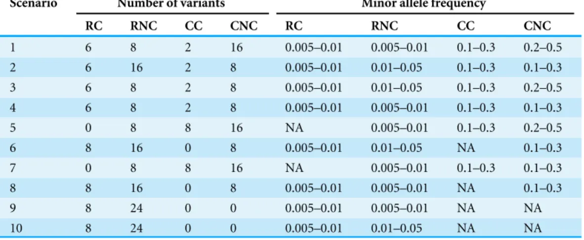
Table 1 Setting of the four types of variantsain 10 scenarios.
Scenario Number of variants Minor allele frequency
RC RNC CC CNC RC RNC CC CNC
1 6 8 2 16 0.005–0.01 0.005–0.01 0.1–0.3 0.2–0.5
2 6 16 2 8 0.005–0.01 0.01–0.05 0.1–0.3 0.1–0.3
3 6 8 2 8 0.005–0.01 0.01–0.05 0.1–0.3 0.2–0.5
4 6 8 2 8 0.005–0.01 0.005–0.01 0.1–0.3 0.1–0.3
5 0 8 8 16 NA 0.005–0.01 0.1–0.3 0.2–0.5
6 8 16 0 8 0.005–0.01 0.01–0.05 NA 0.1–0.3
7 0 8 8 16 NA 0.005–0.01 0.1–0.3 0.1–0.3
8 8 16 0 8 0.005–0.01 0.005–0.01 NA 0.1–0.3
9 8 24 0 0 0.005–0.01 0.005–0.01 NA NA
10 8 24 0 0 0.005–0.01 0.01–0.05 NA NA
Notes.
aRC, rare causal; RNC, rare non-causal; CC, common causal; CNC, common non-causal.
We take ρ=0,0.5 and 0.9 to mimic the no, moderate and strong LD. EachZj is then
transformed to 0 (major allele) or 1 (minor allele) depending on the corresponding MAF of the variant, where MAF is selected from a uniform distribution as shown inTable 1for different scenarios. Simulation of twoZ’s leads to a vector of genotype data denoted as
Xi=(Xi1,...,Xim)′,i=1,...,n. NoteTable 1accommodates different proportions of the
numbers of variants of common to rare, causal to non-causal and varied MAFs. The categorical trait value of the ith subject with genotype Xi is determined by
π1(Xi),...,πK(Xi), which are deduced from the baseline-category logit model (Agresti,
2012) as shown in the previous section. We takeK=3, andα1= −log(4) andα2= −log(3) in the simulation study. To evaluate the type I error rates, we set β1=β2=0 and the nominal significance level α=0.05. For power, we assign various β1 and β2 for both common and rare causal variants, as described in the following, to take different effect sizes and directions into account for investigating the influence of variants on the trait comprehensively. In scenarios 1–4 (see Table 1), the vectorβ1 of effect sizes is (log(3/2),log(1/3),log(3/2),log(3/2),log(1/2),log(1/2)) for the 6 RC variants and (log(11/10),log(2/3)) for the 2 CC variants. Accordingly, the vectorβ2of effect sizes is (log(5/4),log(1/2),log(5/4),log(5/4),log(1/3),log(1/3)) for the 6 RC variants and (log(23/20),log(1/2)) for the 2 CC variants.
In scenarios 6 and 8–10, the vectors β1 andβ2of effect sizes for 8 RC variants are respectively
β′1=(log(5/2),log(1/3),log(11/5),log(11/5),log(11/5),log(1/2),log(1/2),log(1/2)), β′2=(log(7/5),log(1/2),log(2),log(2),log(2),log(1/3),log(1/3),log(1/3)).
In scenarios 5 and 7,β1andβ2for 8 CC variants are respectively
β′1=(log(6/5),log(5/6),log(11/10),log(11/10),log(11/10),log(20/23),
log(20/23),log(20/23)),
Based on these parameter settings, we simulate a pool of 2,000,000 individuals with known multi-site genotypes and categorical trait. A sample ofn=1,000 individuals is randomly chosen from this pool in each of theR=1,000 independent replications. We fix
B=1,000 in the permutation procedure for the calculation ofp-value.
Simulation 2
In this simulation set we increase the numberKof categories to 5 and 8 to make comparison of the test statistics. WhenK=5, we assignα1= −log(2.2),α2= −log(2.1),α3= −log(1.5) andα4= −log(1.2). To evaluate the type I error rates, we setβ1= ··· =β4=0and the nominal significance levelα=0.05. In scenarios 1–4 (seeTable 1), the vectorsβ1 and
β2 of effect sizes are the same as those in Simulation 1. The vectorβ3 of effect sizes is (log(27/20),log(2/5),log(27/20),log(27/20),log(2/5),log(2/5)) for the 6 RC variants and (log(23/20),log(20/23)) for the 2 CC variants. Accordingly, the vectorβ4of effect sizes is (log(17/10),log(10/17),log(17/10),log(17/10),log(10/17),log(10/17)) for the 6 RC variants and (log(6/5),log(5/11)) for the 2 CC variants. In scenarios 6 and 8–10, the vectorsβ1,β2,β3andβ4of effect sizes for 8 RC variants are respectively
β′1=(log(3/2),log(1/3),log(2),log(2),log(2),log(1/2),log(1/2),log(1/2)), β′2=(log(5/4),log(1/2),log(3),log(3),log(3),log(1/3),log(1/3),log(1/3)),
β′3=(log(27/20),log(2/5),log(5/2),log(5/2),log(5/2),log(2/5),log(2/5),log(2/5)), β′4=(log(17/10),log(10/17),log(7/2),log(7/2),log(7/2),log(2/7),log(2/7),log(2/7)).
In scenarios 5 and 7,β1,β2,β3andβ4for 8 CC variants are respectively
β′1=(log(6/5),log(6/5),log(23/20),log(23/20),log(23/20),log(20/23),log(20/23),
log(20/23)),
β′2=(log(23/20),log(1/2),log(28/25),log(28/25),log(28/25),log(25/28),log(25/28),
log(25/28)),
β′3=(log(23/20),log(20/23),log(23/20),log(6/5),log(6/5),log(5/6),log(5/6),log(5/6)), β′4=(log(6/5),log(5/11),log(6/5),log(6/5),log(6/5),log(10/13),log(10/13),log(10/13)).
The other parameter settings refer to Simulation 1.
When K =8, we assign α1= −log(2.2),α2= −log(2.1), α3= −log(1.5), α4= −log(1.6),α5= −log(2),α6= −log(1.8) andα7= −log(2.1). To evaluate the type I error rates, we setβ1= ··· =β7=0and the nominal significance levelα=0.05. In scenarios 1–4 (see Table 1), the vectorβ1of effect sizes is (log(3),log(1/3),log(16/5),log(16/5),
RC variants and (log(23/20),log(20/23)) for the 2 CC variants. The vectorβ6of effect sizes is (log(27/20),log(20/27),log(14/5),log(14/5),log(5/14),log(5/14)) for the 6 RC variants and (log(6/5),log(5/6)) for the 2 CC variants. The vectorβ7 of effect sizes is (log(7/2),log(2/7),log(7/2),log(7/2),log(2/7),log(2/7)) for the 6 RC variants and (log(3/2),log(2/3)) for the 2 CC variants.
In scenarios 6 and 8–10, the vectorsβk(k=1,..,7) of effect sizes for 8 RC variants are respectively
β′1=(log(19/5),log(5/19),log(16/5),log(16/5),log(16/5),log(5/16),
log(5/16),log(5/16)),
β′2=(log(9/2),log(2/9),log(3),log(3),log(3),log(1/3),log(1/3),log(1/3)), β′3=(log(4),log(1/4),log(5/2),log(5/2),log(5/2),log(2/5),log(2/5),log(2/5)), β′4=(log(17/10),log(10/17),log(13/10),log(13/10),log(13/10),log(10/13),
log(10/13),log(10/13)),
β′5=(log(3),log(1/3),log(3),log(3),log(19/5),log(5/19),log(1/3),log(1/3)), β′6=(log(27/20),log(2/5),log(14/5),log(14/5),log(14/5),log(5/14),
log(5/14),log(5/14)),
β′7=(log(7/2),log(2/7),log(7/2),log(7/2),log(7/2),log(2/7),log(2/7),log(2/7)).
In scenarios 5 and 7,βk(k=1,..,7) for 8 CC variants are respectively
β′1=(log(3/2),log(2/3),log(5/4),log(5/4),log(5/4),log(4/5),log(4/5),log(4/5)), β′2=(log(31/20),log(20/31),log(31/20),log(31/20),log(31/20),log(20/31),log(20/31),
log(20/31)),
β′3=(log(23/20),log(20/23),log(23/20),log(23/20),log(23/20),log(20/23),log(20/23),
log(20/23)),
β′4=(log(6/5),log(5/6),log(6/5),log(6/5),log(6/5),log(5/6),log(5/6),log(5/6)), β′5=(log(23/20),log(20/23),log(23/20),log(23/20),log(23/20),log(20/23),log(20/23),
log(20/23)),
β′6=(log(6/5),log(5/6),log(6/5),log(6/5),log(6/5),log(5/6),log(5/6),log(5/6)), β′7=(log(3/2),log(2/3),log(13/10),log(13/10),log(13/10),log(10/13),log(10/13),
log(10/13)).
See Simulation 1 for the other parameter settings.
Simulation 3
Notice in the expressions of β1andβ2in Simulation 1 that 50% of their components are positive. Now we increase this proportion to 75% and 100% and then evaluate the performance of all tests. For demonstration, we choose scenario 10 inTable 1and set
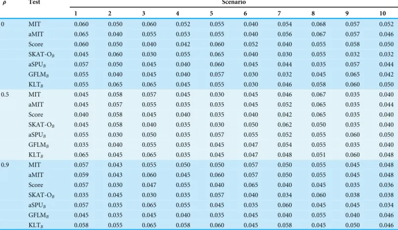
Table 2 Type I error rates of seven tests with 1,000 individuals for the trait with three categories at nominal significance level 0.05.
ρ Test Scenario
1 2 3 4 5 6 7 8 9 10
0 MIT 0.060 0.050 0.060 0.052 0.055 0.040 0.054 0.068 0.057 0.052
aMIT 0.065 0.040 0.055 0.053 0.055 0.040 0.056 0.067 0.057 0.046
Score 0.060 0.050 0.040 0.042 0.060 0.052 0.040 0.055 0.058 0.050
SKAT-OB 0.045 0.060 0.030 0.055 0.065 0.040 0.030 0.055 0.032 0.032
aSPUB 0.057 0.050 0.045 0.040 0.060 0.045 0.044 0.035 0.057 0.044
GFLMB 0.055 0.040 0.045 0.040 0.057 0.030 0.032 0.045 0.065 0.042
KLTB 0.055 0.065 0.065 0.045 0.055 0.030 0.046 0.058 0.060 0.050
0.5 MIT 0.045 0.058 0.057 0.045 0.030 0.045 0.046 0.067 0.035 0.040
aMIT 0.045 0.057 0.055 0.035 0.035 0.045 0.052 0.065 0.035 0.044
Score 0.040 0.058 0.045 0.040 0.035 0.040 0.042 0.065 0.035 0.040
SKAT-OB 0.045 0.058 0.040 0.035 0.030 0.050 0.062 0.050 0.035 0.040
aSPUB 0.055 0.030 0.050 0.035 0.057 0.055 0.052 0.055 0.060 0.050
GFLMB 0.035 0.040 0.055 0.035 0.045 0.047 0.054 0.055 0.035 0.040
KLTB 0.065 0.045 0.065 0.035 0.045 0.047 0.048 0.051 0.060 0.048
0.9 MIT 0.057 0.043 0.055 0.050 0.050 0.057 0.050 0.055 0.045 0.048
aMIT 0.059 0.043 0.060 0.045 0.060 0.057 0.050 0.055 0.045 0.048
Score 0.057 0.030 0.047 0.055 0.040 0.065 0.040 0.045 0.035 0.036
SKAT-OB 0.035 0.045 0.030 0.035 0.057 0.040 0.034 0.060 0.038 0.038
aSPUB 0.057 0.035 0.065 0.055 0.045 0.035 0.060 0.045 0.045 0.034
GFLMB 0.045 0.035 0.045 0.040 0.035 0.045 0.040 0.055 0.040 0.046
KLTB 0.058 0.055 0.065 0.058 0.060 0.045 0.058 0.045 0.050 0.046
in the case of 100% proportion and
β′1=(log(5/2),log(3),log(11/5),log(11/5),log(11/5),log(2),log(1/2),log(1/2)), β′2=(log(7/5),log(2),log(2),log(2),log(2),log(3),log(1/3),log(1/3))
in case of 75%. All the other parameter settings remain the same as Simulation 1.
Simulation results
Type I error rates
To check the validity of our proposed tests MIT and aMIT, in addition to Score, SKAT-OB,
aSPUB, GFLMBand KLTB, we begin by presenting the type I error rates for each test with
the null simulation parameters under different magnitude of LD. The empirical type I error rates of all tests of Simulation 1 and 2 are respectively summarized inTable 2,Table S1(K=5) andTable S2(K=8). These tables demonstrate that the estimated type I error rates of all tests are not significantly different from the predetermined nominal level for different LD amounts. As expected, SKAT-OB, aSPUB, GFLMBand KLTBwere a little bit
less conservative, as can be seen inTable 2,Table S1(K=5) andTable S2(K=8).
Power comparison
Figure 1 Power results of seven tests with 1,000 individuals for a trait with three categories.(A)ρ=0; (B)ρ=0.5; (C)ρ=0.9.
SKAT-O, aSPU and GFLM are implemented by using R packages. The power comparison of these seven tests in Simulation 1 is summarized in Fig. 1. It can be seen from this figure that whenρincreases from 0.5 to 0.9, the power results of MIT and aMIT decrease obviously in scenarios 1–4. This illustrates that the discrepancies between distributions of genetic variants given each categorical trait value decrease when the variants are in strong LD structure. In addition, power results of MIT and aMIT are relatively low in scenarios 6, 8, 9 and 10 with only RC variants. According toFig. 1, aMIT has higher power than MIT for variedρin almost all scenarios. In strong LD structure, the advantage of aMIT becomes more obvious in scenarios 1–4. We could conclude that aMIT is more appropriate when both common and rare causal variants are present in the region of study.
For the four conservative tests SKAT-OB, aSPUB, GFLMB and KLTB, they are not
the winners for all 10 scenarios and 3 LD structures as expected. In scenarios 6 and 8, the performance of SKAT-OB is better than aSPUBor GFLMB. aSPUB or GFLMB has
attracting performance in scenarios 1–5 and 7. The results of power comparison of SKATB
and GFLMB are consistent with those inFan et al. (2014). KLTB is always the winner
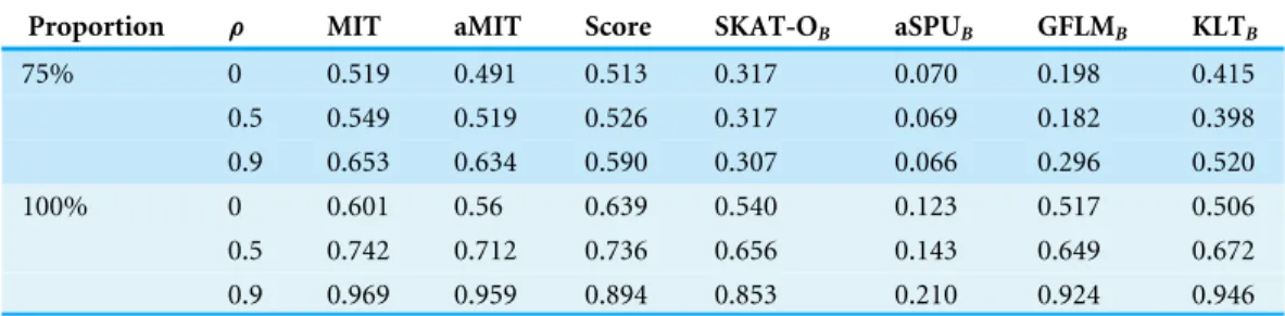
Table 3 Power results of seven tests for 75% and 100% proportions of positive causal variants in causal ones with 1,000 individuals for a trait with three categories at nominal significance level 0.05 in scenario 10.
Proportion ρ MIT aMIT Score SKAT-OB aSPUB GFLMB KLTB
75% 0 0.519 0.491 0.513 0.317 0.070 0.198 0.415
0.5 0.549 0.519 0.526 0.317 0.069 0.182 0.398
0.9 0.653 0.634 0.590 0.307 0.066 0.296 0.520
100% 0 0.601 0.56 0.639 0.540 0.123 0.517 0.506
0.5 0.742 0.712 0.736 0.656 0.143 0.649 0.672
0.9 0.969 0.959 0.894 0.853 0.210 0.924 0.946
the same baseline-category logit model, but it has lower power than KLTB in the other
scenarios. With the exception of scenario 7 with ρ=0.5, either MIT or aMIT is the winner among those seven tests. On average, aMIT is superior to MIT in Simulation 1.
The results of Simulation 2 are shown inFig. S1(K=5) andFig. S2(K=8), and MIT and aMIT tests were almost always the winners. Because the degrees of freedom of the Score test statistic are respectively 4mand 7m(m=24 or 32), the gap between Score and the winner increases when the number of categories increases. Among the four conservative tests, KLTBperforms best whenρ=0 except scenario 9, but does not have high power in
scenarios 4 and 9 withρ=0.5 and in most scenarios withρ=0.9. SKAT-OBperforms
better than aSPUBand GFLMBin scenarios 6, 8 and 10. InFig. S2, the gap between Score
and the winner is noticeable in scenario 9 withρ=0.9. Whenρ=0 and 0.5, KLTBis the
winner among the four conservative tests except scenario 2. aSPUBand GFLMBperform
better than SKAT-OBin scenarios 5 and 7.
The results of Simulation 3 are shown inTable 3. The Simulation 3 focuses on 75% and 100% proportions of positive causal variants with 1,000 individuals. The power of all tests increases with the LD amounts. MIT or aMIT performs better than Score withρ=0.5 and 0.9 in both 75% and 100% cases, but Score is the winner in situation of linkage equilibrium. MIT or aMIT is recommended for the situations in which multiple sites in a region are in, weak or strong, LD.
It is demonstrated for the most situations inFig. 1,Figs. S1,S2andTable 3that the performance of MIT or aMIT is superior to the existing methods in term of detecting variants. For scenarios shown in Fig. 1,Figs. S1 andS2, aMIT performs better than MIT, especially for big LD amounts or they have approximately equal power. When the proportion of positive causal variants increases as shown in Table 3, MIT has some advantages. In summary, MIT and aMIT have superior performance in a range of scenarios, compared to several existing tests.
Application to data from collaborative study on the genetics of alcoholism study
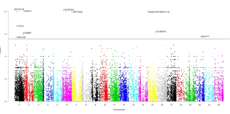
Figure 2 The manhattan plot of allp-values of genes based on MIT for COGA data.Horizontal black line represents the threshold of 2.798×10⁻⁶.
group. All subjects were tested through the Semi-Structured Assessment for the Genetics in Alcoholism (Bucholz et al.,1994).
Genotyping was sequenced by the Illumina Human 1M DNA Analysis at the Center for Inherited Disease Research. The sequence data contain 1,072,820 SNPs in 18,946 genes on all chromosomes. There are 32 subjects for which phenotypes are released, but no genotype data is available, so they are removed in the subsequent analyses. After removing variants that have no sequence variation (all homozygous for the common allele), there are 17,868 genes on autosomes with 1,913 subjects.
ALDX1 (Alcohol diagnosis—DSM3R (American Psychiatric Association, 1994) and
Feighner et al. (1972) is a categorical trait with three categories (1-pure unaffected, 3-unaffected with some symptoms and 5-affected) in COGA data, which depicts the severity of alcohol dependence. The data used for analyzing are collected from dbGaP at http://www.ncbi.nlm.nih.gov/projects/gap/cgi-bin/study.cgi?study_id=phs000125.v1.p1 through dbGaP accession numberphs000125.v1.p1. A number of researchers involve in this study and they analyze SNP one by one or one whole chromosome or utilize other related traits (Edenberg et al.,2010;Zhang, Liu & Wang,2010;Wang et al.,2011). We utilize ALDX1 to reanalyze COGA data and detect genes associated with ALDX1.
A genome-wide scan
and we have skipped them here. Due to the time limitation in the permutation procedure, thep-values of less than 10−8will be denoted by−log(10−8)=8 inFig. 2. It is concluded fromFig. 2that there are a total of 10 significant genes.
We are interested in the functions of these significant genes and their relationships with alcohol dependence. Gene PPP1R12B, also known as MYPT2, is a subunit of protein phosphatase 1 (PP1) and is mainly reflected in the heart, skeletal muscle and the brain (Pham et al.,2012). There is no doubt that the problem of binge drinking, particularly by young, needs to be addressed urgently, to prevent cognitive impairment, which could lead to irreversible brain damage (Ward, Lallemand & De witte,2009). In the neural development stage, different ethanol treatments can change the expression of gene PPP1R12B in the adult brain (Kleiber et al., 2013). PP1 is in the alcoholism pathway for human; seeFigs. S3from the Kyoto Encyclopedia of Genes and Genomes (KEGG) (http://www.genome.jp/dbget-bin/www_bget?map05034). N-methyl-D-aspartate (NMDA) receptor which is a glutamate receptor and ion channel protein can be dephosphorylated by PP1. DARPP32 (dopamine- and cAMP-regulated phosphoprotein of 32 kDa) is a protein expressed mainly in neurons and restrains PP1. DARPP32 augments NMDA receptor phosphorylation, which adds channel function and offsets acute prohibition about ethanol (Spanagel,2009). PP1 plays the role of a bridge between NMDA and DARPP32. The relationship between alcohol, dopamine and glutamate may be likely to develop ‘‘binge drinking’’ (alcoholism) (Ward, Lallemand & De witte,2009).
Gene HIST1H2AI is one of the histone H2A family. H2A is also in the alcoholism pathway (see Figs. S3). The position of Histones is very important in transcription regulation, the repair and recombination of DNA and the stability of chromosome. A complex set of histone repair regulate DNA, which are also known as histone codes, and the rebuilding of nucleosome (http://www.genecards.org/cgi-bin/carddisp.pl?gene= HIST1H2AI&keywords=HIST1H2AI). The histone octamer contains two molecules of each of the histones H2A, H2B, H3 and H4, around which the DNA wraps (Mandrekar,
2011). For alcoholism, the roles of Histone acetylation and methylation are very important in brain and peripheral tissues (Starkman, Sakharkar & Pandey,2012).
The brain could be affected by alcoholism which results in tolerance and dependence. Moreover alcoholism will have a serious harmful effects in other organs. PPIAL4A is a protein-coding gene and associates with liver cancer ( http://www.genecards.org/cgi-bin/carddisp.pl?gene=PPIAL4A&keywords=PPIAL4A).
In addition, nicotine use is closely related with ethanol intake. Smokers will be prone to drink more ethanol than the peers of nonsmokers (Britt & Bonci,2013). Drinkers are very liable to smoke; moreover, alcoholics are often dependent on tobacco (Drobes,
2002). Gene CHRNB2 is in nicotine addiction pathway. Moreover, CHRNB2 associates with tobacco- and ethanol-associated traits, and markers mediating early responses to nicotine and alcohol can be found in CHRNB2 (Ehringer et al.,2007). C20orf111 resides in marker D20S119, which has a high LOD score using the alcoholism phenotype (Hill et al.,2004).
believed to compromise immune function and the nervous system (Silverstein & Kumar,
2014). In fact, the progression of HIV may be aggravated by alcohol abuse and HIV patients are more likely to use alcohol than the general subjects (Pandrea et al.,2010).
Functional genes
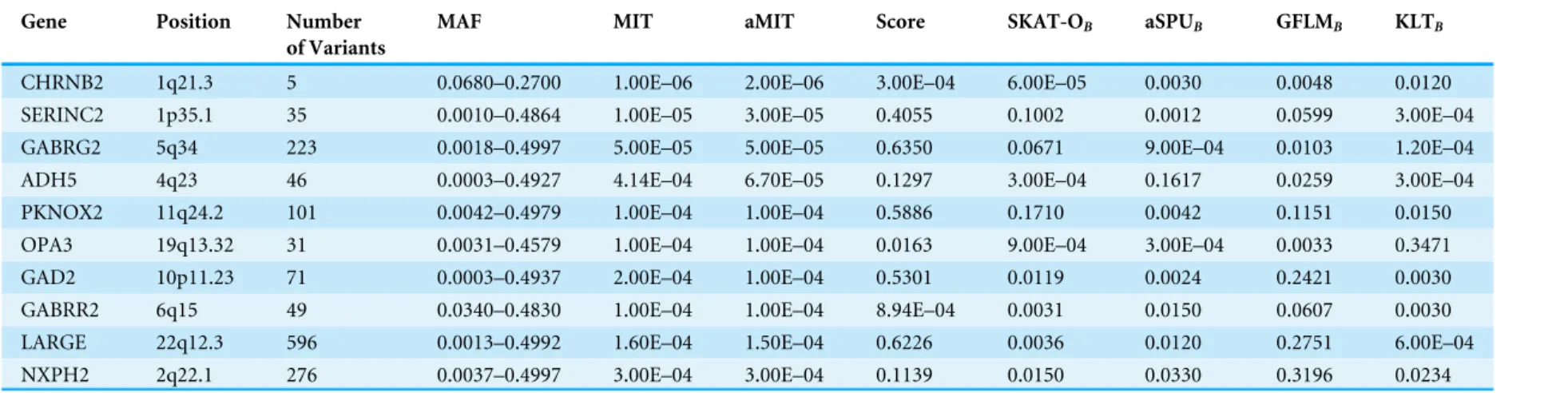
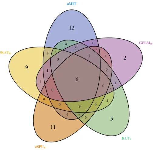
For comparison of all tests, we focus on functional genes as shown in literatures. There are a total of 304 genes associated with alcohol dependence based on National Center for Biotechnology Information (http://www.ncbi.nlm.nih.gov/). From them, we select 202 functional genes which are for human sapiens and are present in COGA data. Top 10 genes detected by aMIT are shown inTable 4. It is apparent that MIT or aMIT performs much better than other tests. Note for the MAF shown in the third column inTable 4that there are both rare and common variants in these genes. Meanwhile,Figure 3depicts a five-way Venn diagram illustrating either the concordance or discordance of genes found to be significant withp-values less than 0.05 for five tests. The counts shown where all ellipses overlap indicate the number of (concordant) genes which are detected by all tests, while the counts that are in only one ellipse denote the number of (discordant) genes that are detected by the corresponding test. The counts of each ellipse for aMIT, Score, SKAT-OB,
aSPUB, GFLMB and KLTBtests are respectively 90, 21, 46, 52, 34 and 68. As the Score
test only detects 21 functional genes and is excluded in Venn diagram. There are six genes detected by all five tests inFig. 3. It is concluded from this figure that aMIT test is the most powerful tool to detect functional genes.
Alcohol dependence can affect our brain, heart, immune system, and even our life. Long-term use of alcohol can cause serious health complications, affecting almost most of the organs in our body. The MIT or aMIT tests perform better than other tests for detecting the association between function genes and categorical traits.
DISCUSSION
In the era of GWASs, tremendous efforts are devoted to developing methods for investigating genetic variants associated with quantitative/binary/ordinal traits. It seems true that the categorical trait receives little attention. One possible reason for this is the lack of appropriate/powerful statistical method. Although the conventional baseline-category logit model could be used to explore the relationship between multiple variants and categorical trait, it would suffer from low power when the number of variants/categories increases, or in some situations we do not have sufficient reasons to use this model to fit the observed data. It is desirable to develop nonparametric test with high power to deal with categorical traits.
Table 4 The top 10 genes detected by aMIT in 202 functional genes.
Gene Position Number
of Variants
MAF MIT aMIT Score SKAT-OB aSPUB GFLMB KLTB
CHRNB2 1q21.3 5 0.0680–0.2700 1.00E–06 2.00E–06 3.00E–04 6.00E–05 0.0030 0.0048 0.0120
SERINC2 1p35.1 35 0.0010–0.4864 1.00E–05 3.00E–05 0.4055 0.1002 0.0012 0.0599 3.00E–04
GABRG2 5q34 223 0.0018–0.4997 5.00E–05 5.00E–05 0.6350 0.0671 9.00E–04 0.0103 1.20E–04
ADH5 4q23 46 0.0003–0.4927 4.14E–04 6.70E–05 0.1297 3.00E–04 0.1617 0.0259 3.00E–04
PKNOX2 11q24.2 101 0.0042–0.4979 1.00E–04 1.00E–04 0.5886 0.1710 0.0042 0.1151 0.0150
OPA3 19q13.32 31 0.0031–0.4579 1.00E–04 1.00E–04 0.0163 9.00E–04 3.00E–04 0.0033 0.3471
GAD2 10p11.23 71 0.0003–0.4937 2.00E–04 1.00E–04 0.5301 0.0119 0.0024 0.2421 0.0030
GABRR2 6q15 49 0.0340–0.4830 1.00E–04 1.00E–04 8.94E–04 0.0031 0.0150 0.0607 0.0030
LARGE 22q12.3 596 0.0013–0.4992 1.60E–04 1.50E–04 0.6226 0.0036 0.0120 0.2751 6.00E–04
NXPH2 2q22.1 276 0.0037–0.4997 3.00E–04 3.00E–04 0.1139 0.0150 0.0330 0.3196 0.0234
Notes.
MAF, minor allele frequency.
Sun
e
t
al.
(2016),
P
eerJ
,
DOI
Figure 3 The Venn diagram of the counts of genes found significant withp-value less than 0.05 for five tests from 202 funtional genes.
CONCLUSION
In this paper, we develop MIT and aMIT, two nonparametric tests which can effectively detect the association between genetic variants and categorical traits. One feature of MIT or aMIT is that they are free of models. Observed from simulation studies and real data analyses, the proposed tests perform better than the conventional Score test. Therefore, MIT and aMIT are recommended for identifying genetic variants associated with categorial traits.
ACKNOWLEDGEMENTS
The authors would like to thank the Academic Editor and anonymous reviewers for their insightful and constructive comments, which lead to an improved manuscript.
APPENDIX. SCORE TEST STATISTIC
In this appendix, we sketch the derivation of score test statistic for testingH0:β1=β2= ··· =βK−1=0based on the following baseline-category logit model:
logπk(Xi)
πK(Xi)
=αk+X′iβk, k=1,...,K−1,i=1,...,n,
which implies πK(Xi)= [1+PK−k=11exp(αk+X′iβk)]−1 for everyi. For subject i, let
(yi1,...,yiK)′ represent his/her multinomial trait, where yik=1 when the trait is in
category k, andyik=0 otherwise, so PKk=1yik=1. SinceπK =1−(π1+ ··· +πK−1)
andyiK=1−(yi1+ ··· +yi,K−1), the log likelihood function (Agresti,2012) is
l=log
n Y i=1 " K Y k=1
πk(Xi)yik #
=
n X
i=1
"K−1
X
k=1
yiklogπk(Xi)+(1− K−X1
k=1
yik)logπK(Xi) #
=
n X
i=1
"K−1
X
k=1
yiklog
πk(Xi)
πK(Xi)
+logπK(Xi) #
=
n X
i=1
K−X1
k=1
yik(αk+Xi′βk)− n X i=1 log(1+ K−1 X
k=1
exp(αk+X′iβk)).
The first partial derivatives of the log likelihood with respect to parameters αk and
βk (1≤k≤K−1) are respectively
∂l ∂αk = n X i=1
yik− n X
i=1
πK(Xi)exp(αk+X′iβk),
∂l
∂βk =
n X
i=1
yikXi−
n X
i=1
πK(Xi)exp(αk+Xi′βk)Xi.
Under H0, the maximum likelihood estimatorsbαk of unknown parametersαk(1≤k≤
K−1) can be solved from the followingK−1 equations
∂l ∂αk H0
which can be simplified to[1+PK−k=11exp(αk)]−1exp(αk)=y·k,wherey·k=1n1′yk,1is the
all 1 vector of lengthn, andyk=(y1k,y2k,...,ynk)′,k=1,..,K−1.
The score vectorU=(U′
1,...,U′K−1)′, whereUk is∂l/∂βk evaluated atH0andαk=bαk,
k=1,...,K−1. Based on the expression of∂l/∂βk, we have
Uk=
n X
i=1
(yik−y·k)Xi=X′(In−
1
n11
′)yk,
whereX′=(X1,...,Xn) andIn is then×nidentity matrix. Note that whenH0 holds and αk =bαk, we have Cov(yk,yk)=y·k(1−y·k)In andCov(yk,yk′)= −y·ky·k′In, for
1≤k6=k′≤K−1. So the corresponding variance–covariance matrixVofUis
y·1(1−y·1) −y·1y·2 ··· −y·1y·K−1
−y·2y·1 y·2(1−y·2) ··· −y·2y·K−1
..
. ... ... ...
−y·K−1y1 −y·K−1y·2 ··· y·K−1(1−y·K−1)
⊗X′(In−1
n11
′)X,
where⊗is the matrix Kronecker product. The score test statistic isU′V−1Uwhich has an asymptoticχ2distribution withrank(V) degrees of freedom.
ADDITIONAL INFORMATION AND DECLARATIONS
Funding
This research was supported in part by the National Natural Science Foundation of China (11571082, 11171075), National Basic Research Program of China (2012CB316505), and the Scientific Research Foundation of Fudan University. The funders had no role in study design, data collection and analysis, decision to publish, or preparation of the manuscript.
Grant Disclosures
The following grant information was disclosed by the authors: National Natural Science Foundation of China: 11571082, 11171075. National Basic Research Program of China: 2012CB316505.
Scientific Research Foundation of Fudan University.
Competing Interests
The authors declare there are no competing interests.
Author Contributions
• Leiming Sun conceived and designed the experiments, performed the experiments, analyzed the data, contributed reagents/materials/analysis tools, wrote the paper, prepared figures and/or tables.
• Yue-Qing Hu conceived and designed the experiments, performed the experiments, analyzed the data, wrote the paper, prepared figures and/or tables, reviewed drafts of the paper.
Data Availability
The following information was supplied regarding data availability:
CIDR: Collaborative Study on the Genetics of Alcoholism Case Control Study; dbGaP Study Accession:phs000125.v1.p1;http://www.ncbi.nlm.nih.gov/projects/gap/ cgi-bin/study.cgi?study_id=phs000125.v1.p1.
Supplemental Information
Supplemental information for this article can be found online athttp://dx.doi.org/10.7717/ peerj.2139#supplemental-information.
REFERENCES
Agresti A. 2012.Categorical data analysis. Hoboken: Wiley.
American Psychiatric Association. 1994.Diagnostic and statistical manual of mental disorders. Washington, D.C: American Psychiatric Association.
Britt J, Bonci A. 2013.Alcohol and tobacco: how smoking may promote excessive drinking.Neuron79(3):406–447DOI 10.1016/j.neuron.2013.07.018.
Brunel H, Gallardo-Chacón JJ, Buil A, Vallverdú M, Soria JM, Caminal P, Perera A. 2010.MISS: a non-linear methodology based on mutual information for genetic association studies in both population and sib-pairs analysis.Bioinformatics
26(15):1811–1818DOI 10.1093/bioinformatics/btq273.
Bucholz KK, Cadoret R, Cloninger CR, Dinwiddie SH, Hesselbrock VM, Nurnberger JJ, Reich T, Schmidt I, Schuckit MA. 1994.A new, semi-structured psychiatric interview for use in genetic linkage studies: a report on the reliability of the SSAGA.
Journal of Studies on Alcohol55(2):149–158DOI 10.15288/jsa.1994.55.149.
Dawy Z, Goebel B, Hagenauer J, Andreoli C, Meitinger T, Mueller JC. 2006.
Gene mapping and marker clustering using shannon’s mutual information.
IEEE/ACM Transactions on Computational Biology and Bioinformatics3(1):47–56 DOI 10.1109/TCBB.2006.9.
Drobes DJ. 2002.Concurrent alcohol and tobacco dependence: mechanisms and treatment.Alcohol Research and Health26:136–142.
Edenberg HJ, Koller DL, Xuei XL, Wetherill L, McClintick JN, Almasy L, Bierut LJ, Bucholz KK, Goate A, Aliev F. 2010.Genome-wide association study of alcohol dependence implicates a region on chromosome 11.Alcoholism: Clinical and Experimental Research34(5):840–852DOI 10.1111/j.1530-0277.2010.01156.x.
Ehringer MA, Clegg HV, Collins AC, Corley RP, Crowley T, Hewitt JK, Hopfer CJ, Krauter K, Lessem J, Rhee SH. 2007.Association of the neuronal nicotinic receptor
Fan R, Wang Y, Mills JL, Carter TC, Lobach I, Wilson AF, Bailey-Wilson JE, Weeks DE, Xiong M. 2014.Generalized functional linear models for gene-based case-control association studies.Genetic Epidemiology38(7):622–637DOI 10.1002/gepi.21840.
Fan R, Wang Y, Mills JL, Wilson AF, Bailey-Wilson JE, Xiong M. 2013.Functional linear models for association analysis of quantitative traits.Genetic Epidemiology
37(7):726–742DOI 10.1002/gepi.21757.
Fan R, Zhong M, Wang S, Zhang Y, Andrew A, Karagas M, Chen H, Amos C, Xiong M, Moore J. 2011.Entropy-based information gain approaches to detect and to characterize gene–gene and gene-environment interactions/correlations of complex diseases.Genetic Epidemiology35(7):706–721 DOI 10.1002/gepi.20621.
Feighner JP, Robins E, Guze SB, Woodruff RA, Winokur G, Munoz R. 1972.Diagnostic criteria for use in psychiatric research.Archives of General Psychiatry26:57–63 DOI 10.1001/archpsyc.1972.01750190059011.
Hill SY, Shen S, Zezza N, Hoffman EK, Perlin M, Allan W. 2004.A genome wide search for alcoholism susceptibility genes.American Journal of Medical Genetics Part B: Neuropsychiatric Genetics128B(1):102–113DOI 10.1002/ajmg.b.30013.
Kim ES, Yoon M. 2011.Testing measurement invariance: a comparison of multiple-group categorical CFA and IRT.Structural Equation Modeling A Multidisciplinary Journal 18(2):212–228DOI 10.1080/10705511.2011.557337.
Kleiber ML, Mantha K, Stringer RL, Singh SM. 2013.Neurodevelopmental alcohol exposure elicits long-term changes to gene expression that alter distinct molecular pathways dependent on timing of exposure.Journal of Neurodevelopmental Disorders
5(6):1–19DOI 10.1186/1866-1955-5-1.
Kullback S, Leibler RA. 1951.On information and sufficiency.Annals of Mathematical Statistics22:79–86DOI 10.1214/aoms/1177729694.
Lee S, Wu MC, Lin X. 2012.Optimal tests for rare variant effects in sequencing associa-tion studies.Biostatistics13(4):762–775DOI 10.1093/biostatistics/kxs014.
Madsen BE, Browning SR. 2009.A groupwise association test for rare mutations using a weighted sum statistic.PLoS Genetics5(2):e1000384
DOI 10.1371/journal.pgen.1000384.
Mandrekar P. 2011.Epigenetic regulation in alcoholic liver disease.World Journal of Gastroenterology17(20):2456–2464DOI 10.3748/wjg.v17.i20.2456.
Manolio TA, Collins FS, Cox NJ, Goldstein DB, Hindorff LA, Hunter DJ, Mccarthy MI, Ramos EM, Cardon LR, Chakravarti A, Cho JH, Guttmacher AE, Kong A, Kruglyak L, Mardis E, Rotimi CN, Slatkin M, Valle D, Whittemore AS, Boehnke M, Clark AG, Eichler EE, Gibson G, Haines JL, Mackay TF, McCarroll SA, Visscher PM. 2009.Finding the missing heritability of complex diseases.Nature
461(7265):747–753DOI 10.1038/nature08494.
Morgenthaler S, Thilly WG. 2007.A strategy to discover genes that carry multi-allelic or mono-allelic risk for common diseases: a cohort allelic sums test (CAST).Mutation Research615(1–2):28–56DOI 10.1016/j.mrfmmm.2006.09.003.
Pan W, Kim J, Zhang Y, Shen X, Wei P. 2014.A powerful and adaptive association test for rare variants.Genetics197(4):1081–1095DOI 10.1534/genetics.114.165035.
Pandrea I, Happel KI, Amedee AM, Bagby GJ, Nelson S. 2010.Alcohol’s role in HIV transmission and disease progression.Alcohol Research and Health World
33(3):203–218.
Pham K, Langlais P, Zhang X, Chao A, Zingsheim M, Yi Z. 2012.Insulin-stimulated phosphorylation of protein phosphatase 1 regulatory subunit 12B revealed by HPLC-ESI-MS/MS.Proteome Science10(1):1122–1136DOI 10.1186/1477-5956-10-52.
Silverstein PS, Kumar A. 2014.HIV-1 and alcohol: interactions in the central ner-vous system.Alcoholism: Clinical and Experimental Research38(3):604–610 DOI 10.1111/acer.12282.
Spanagel R. 2009.Alcoholism: a systems approach from molecular physiology to addic-tive behavior.Physiological Reviews89(2):649–705DOI 10.1152/physrev.00013.2008.
Starkman BG, Sakharkar AJ, Pandey SC. 2012.Epigenetics-beyond the genome in alcoholism.Alcohol Research34(3):293–305.
Turkmen AS, Yan Z, Hu YQ, Lin S. 2015.Kullback-leibler distance methods for detect-ing disease association with rare variants from sequencdetect-ing data.Annals of Human Genetics79(3):199–208DOI 10.1111/ahg.12103.
Wang KS, Liu X, Zhang Q, Pan Y, Aragam N, Zeng M. 2011.A meta-analysis of two genome-wide association studies identifies 3 new loci for alcohol dependence.
Journal of Psychiatric Research45(11):1419–1425 DOI 10.1016/j.jpsychires.2011.06.005.
Ward RJ, Lallemand F, De witte P. 2009.Biochemical and neurotransmitter changes implicated in alcohol-induced brain damage in chronic or ‘binge drinking’ alcohol abuse.Alcohol and Alcoholism44(2):128–135DOI 10.1093/alcalc/agn100.
Wu MC, Lee S, Cai T, Li Y, Boehnke M, Lin X. 2011.Rare-variant association testing for sequencing data with the sequence kernel association test.American Journal of Human Genetics89(1):82–93DOI 10.1016/j.ajhg.2011.05.029.
Yi N, Zhi D. 2011.Bayesian analysis of rare variants in genetic association studies.Genetic Epidemiology 35(1):57–69DOI 10.1002/gepi.20554.
Zhang H, Liu CT, Wang X. 2010.An association test for multiple traits based on the generalized kendall’s tau.Journal of the American Statistical Association
105(490):473–481DOI 10.1198/jasa.2009.ap08387.