© Author(s) 2006. This work is licensed under a Creative Commons License.
Chemistry
and Physics
Modelling study of the impact of deep convection on the utls air
composition – Part I: Analysis of ozone precursors
V. Mar´ecal1, E. D. Rivi`ere1,*, G. Held2, S. Cautenet3, and S. Freitas4
1Laboratoire de Physique et Chimie de l’Environnement/CNRS and Universit´e d’Orl´eans, 3A Avenue de la Recherche
Scientifique, 45 071 Orl´eans cedex 2, France
2Instituto de Pesquisas Meteorol´ogicas, Universidade Estadual Paulista, CX Postal 281 17033-360 Bauru, S.P., Brazil 3Laboratoire de M´et´eorologie Physique/CNRS-OPGC/Universit´e Blaise Pascal, 24 Avenue des Landais, 63 177 Aubi`ere
cedex, France
4Centro de Previs˜ao de Tempo e Estudos Clim`aticos, Rodovia Presidente Dutra, km 40 SPRJ 12630-000, Cachoeira Paulista –
SP, Brazil
*now at: Groupe de Spectrom´etrie Mol´eculaire et Atmosph´erique UMR 6089 and Universit´e de Reims Champagne-Ardenne,
Facult´e des Sciences, Bˆat. 6, case 36, BP 1039, 51 687 Reims Cedex 2, France
Received: 10 November 2004 – Published in Atmos. Chem. Phys. Discuss.: 23 September 2005 Revised: 6 February 2006 – Accepted: 15 March 2006 – Published: 18 May 2006
Abstract. The aim of this work is to study the local impact on the upper troposphere/lower stratosphere air composition of an extreme deep convective system. For this purpose, we performed a simulation of a convective cluster composed of many individual deep convective cells that occurred near Bauru (Brazil). The simulation is performed using the 3-D mesoscale model RAMS coupled on-line with a chemistry model. The comparisons with meteorological measurements show that the model produces meteorological fields generally consistent with the observations.
The present paper (part I) is devoted to the analysis of the ozone precursors (CO, NOxand non-methane volatile
or-ganic compounds) and HOxin the UTLS. The simulation
re-sults show that the distribution of CO with altitude is closely related to the upward convective motions and consecutive outflow at the top of the convective cells leading to a bulge of CO between 7 km altitude and the tropopause (around 17 km altitude). The model results for CO are consistent with satellite-borne measurements at 700 hPa. The simula-tion also indicates enhanced amounts of NOxup to 2 ppbv in
the 7–17 km altitude layer mainly produced by the lightning associated with the intense convective activity. For insolu-ble non-methane volatile organic compounds, the convective activity tends to significantly increase their amount in the 7– 17 km layer by dynamical effects. During daytime in the presence of lightning NOx, this bulge is largely reduced in
the upper part of the layer for reactive species (e.g. isoprene, ethene) because of their reactions with OH that is increased
Correspondence to:V. Mar´ecal ([email protected])
on average during daytime. Lightning NOxalso impacts on
the oxydizing capacity of the upper troposphere by reducing on average HOx, HO2, H2O2 and organic hydroperoxides.
During the simulation time, the impact of convection on the air composition of the lower stratosphere is negligible for all ozone precursors although several of the simulated convec-tive cells nearly reach the tropopause. There is no signifi-cant transport from the upper troposphere to the lower strato-sphere, the isentropic barrier not being crossed by convec-tion.
The impact of the increase of ozone precursors and HOx
in the upper troposphere on the ozone budget in the LS is discussed in part II of this series of papers.
1 Introduction
tropopause and the surface emissions only reach the tropi-cal tropopause layer (TTL). Several definitions for the TTL have been proposed in the literature. We will retain hereafter the following: TTL is the transitional layer between air hav-ing tropospheric characteristics and air havhav-ing stratospheric characteristics. The TTL extends from about 12–14 km to about 17–20 km altitude. From this layer, the air is then en-tering the stratosphere through slow radiative heating ascent. Therefore, the impact of the tropical deep convection on the redistribution of chemical species in the TTL is an important issue in the understanding of the stratospheric ozone budget at global scale.
Several modelling studies (e.g., Wang et al., 1996; Tulet et al., 2002 and Wang and Prinn, 2000) have shown that a deep convective event significantly redistributes all chemi-cal species in the vertichemi-cal. In particular, the convective up-drafts lift rapidly the pollutants emitted at the surface up to the UT where they are horizontally spread by the convective outflow. Apart from its dynamical effect, convection also modifies the chemical budget of the troposphere in particu-lar by scavenging soluble species and by aqueous chemistry (e.g., Mari et al. 2000; Yin et al. 2001; Wang and Prinn, 2000; Barth et al. 2001). Since the modelling of these pro-cesses is fairly complex, each of these studies focused on a particular aspect of the interaction between the microphysics and the chemistry. In particular, Mari et al. (2000) estimated quantitatively the scavenging efficiency in a deep convective event over Brazil for soluble species. In parallel, Barth et al. (2001) investigated the fate of tracers of varying solubili-ties when liquid hydrometeors are converted to ice and Wang and Prinn (2000) showed the importance of aqueous chem-istry for a tropical maritime convective cloud in the total sul-fate production. Another process affecting the air composi-tion and related to deep conveccomposi-tion is the produccomposi-tion of NOx
through lightning (e.g., Wang and Prinn, 2000; DeCaria et al., 2005). In particular, Wang and Prinn (2000) showed that the lightning NOxis very important in the O3chemistry via
chemistry and modification of UV fluxes. For its case study, DeCaria et al. (2005) found an ozone production of 10 ppbv that can be attributed to lightning NO in the UT.
Although tropical regions are of major importance for stratospheric ozone, there have been only few field cam-paigns in the tropics documenting the tropical Upper Tro-posphere and Lower Stratosphere (UTLS). There is still a need for measurements of both tropospheric and strato-spheric species in the whole altitude range of the tropical UTLS in the vicinity of convective events to improve our un-derstanding of the impact of deep convection on the UTLS air composition. Nevertheless, the recent interest of the sci-entific community for the tropical UTLS has led to the design of a major field experiment in Brazil within the framework of the HIBISCUS (Impact of Tropical Convection on the Up-per Troposphere and Lower Stratosphere at Global Scale), TroCCiNOx(Tropical Convection, Cirrus and Nitrogen
Ox-ides) and TroCCiBras (Tropical Convection and Cirrus
ex-periment Brasil) projects. The scientific objective common to the three projects is to study the interaction between mete-orological, atmospheric chemistry and lightning parameters in tropical convection between ground level and the lower stratosphere in Eastern Brazil and in particular in the Bauru region (State of S˜ao Paulo in Brazil). The main field cam-paign of these coordinated projects took place during Febru-ary and March 2004. The present study was done within the frame of the preparation for this campaign.
Central and Eastern Brazil have already been in the past the scene of a few field campaigns during the wet season, providing airborne and balloon-borne measurements of trace gases and water vapour in the troposphere and in the LS. The main airborne experiments were the TROPOZ II (Tropo-spheric Ozone) experiment that took place in January 1991 (Marenco et al., 1995) and the TRACE A (Transport and At-mospheric Chemistry Near the Equator-Atlantic) experiment that took place during the dry (September/October) and the wet (April) seasons in 1992 (Fishman et al., 1996). In par-allel, balloon-borne instruments were flown in Central and Eastern Brazil mainly performing measurements of ozone (Kirchhoff et al., 1996; Logan, 1999; Pundt et al., 2002; V¨omel et al., 2002; Thompson et al., 2003). One of the most outstanding results from these observational studies was, that there is a large increase of the ozone mixing ratio with alti-tude starting in the UT well below the tropopause (Logan, 1999; Pundt et al., 2002; Thompson et al., 2003). The start-ing altitude for this ozone increase is located at the basis of the TTL and varies from about 13 to 16 km. As for ozone precursors, an upper tropospheric maximum for CO mixing ratios was also found above 7 km altitude by Jonqui`eres and Marenco (1998) from TROPOZ II airborne observations dur-ing the wet season. They showed that this maximum was re-lated to the uplifting of surface emissions by convective pro-cesses. These studies and others (e.g., V¨omel et al., 2002) show that the TTL is characterized by a specific air compo-sition, in particular during the wet season.
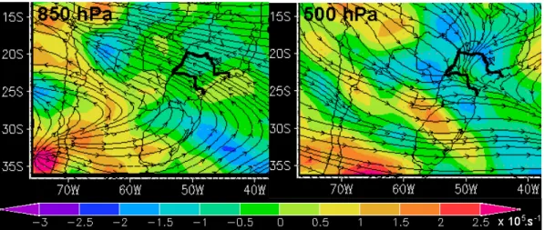
Fig. 1.8 February 2001 at 00:00 UT: Streamflow lines and divergence (in s−1)at 850 hPa (left panel) and 500 hPa (right panel), with borders of the State of S˜ao Paulo shown in bold, from CPTEC Global analysis.
Modeling System) (Cotton et al., 2003) coupled with on-line chemistry and emission modules. This tool allows the quan-tification of the impact of vertical transport, the horizontal transport, as well as lightning NOx, gaseous and aqueous
chemistry on the air composition. The present paper is the first part of a series of two. It is mainly devoted to the anal-ysis of the results for ozone precursors: CO, NOxand
non-methane volatile organic compounds (NMVOC). The second part of the series (Rivi`ere et al., 2006) studies ozone based on the results discussed in Part I. In Sect. 2 of the present paper, a description of the case study is given. Details on the model used to perform the simulation are given in Sect. 3. The simulation results for the meteorological parameters are evaluated in Sect. 4. They are compared to the data col-lected by near-surface observational stations and to the ob-servations from the Bauru radar. The simulation results for ozone precursors are shown and discussed in Sect. 5. They are compared with the airborne and balloon-borne measure-ments performed in Eastern Brazil and published in the liter-ature and with satellite observations of CO over Brazil. Par-ticular attention is given to the impact of the production of NOxby lightning on the other ozone precursors in the
con-vective area. The results for HOxand its precursors are
anal-ysed in Sect. 6. The conclusion of this study is summarised in Sect. 7.
2 Description of the case study
The beginning of February 2001 was characterized by a syn-optic situation typical for summer in the State of S˜ao Paulo. In broad terms, it can be summed up by a high pressure sys-tem situated off the coast between the State of S˜ao Paulo and southern Brazil and ridging in over the continent, with a weak cold front extending along its northern flank across Rio de Janeiro into Minas Gerais. The other component was a
large cyclone initially centred over north-western Argentina from where a tongue of moist air extended across Paraguay, Paran´a and the State of S˜ao Paulo into Mato Grosso do Sul. Another important fact was the strong confluence of wind in the 700 hPa level over the State of S˜ao Paulo, overlaid by an exceptionally strong divergence at levels from 500 hPa upwards. The deep cyclone, which had developed over the southern part of the continent on 6 February 2001 had drasti-cally intensified while moving south-eastwards, pushing the anticyclone eastwards off the central part of the continent and towards the ocean. A more detailed description of the syn-optic situation is given in Held and Nachtigall (2002). On 8 February 2001 at 00:00 UT, an extremely strong conflu-ence of moist maritime air was observed near the surface over the State of S˜ao Paulo at the 850 hPa level, overlaid by a very strong inflow of tropical air at 500 hPa (see Fig. 1), and topped by significant divergence at 300 hPa.
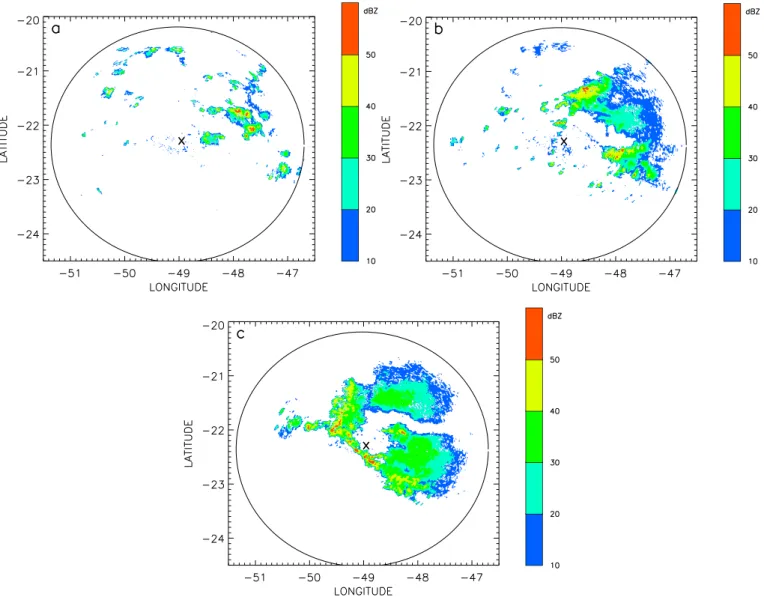
Fig. 2.Radar reflectivity in dBZ from the Bauru radar at 1.7◦elevation with a 240 km range(a)at 18:00 UT,(b)20:00 UT and(c)22:00 UT.
The cloud tops derived from the radar volume scans during the convective event showed that the most intense cells of the system generally reached 15–16 km altitude (not shown). A small proportion of them were penetrating the tropopause up to 18–19 km altitude.
3 Numerical model
The model used in the present study is called hereafter the “RAMS-Chemistry” model. It is composed of the Re-gional Atmospheric Modeling System (RAMS) coupled on-line with a chemistry model. RAMS (Pielke et al., 1992) is a primitive equation prognostic model that simulates three-dimensional atmospheric circulations and weather systems. The RAMS version used in this study is the 4.3 version (Cot-ton et al., 2003). RAMS has a multiple grid nesting scheme solving the model equations simultaneously on interacting
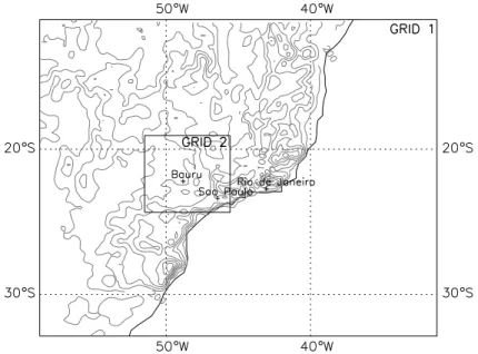
computational meshes of differing spatial resolution (Clark and Farley, 1984; Clark and Hall, 1991, Walko et al., 1995a). The simulation discussed in the present paper includes two grid areas that are illustrated in Fig. 3. The coarse grid (Grid 1) covers a 3000 km by 2500 km domain from 60.8◦W to 29.2◦W in longitude and from 10.8◦S to 32.7◦S in lat-itude. Its horizontal grid spacing is 20 km. The fine grid (Grid 2) domain is 628 km by 608 km with a 4 km grid spac-ing. Grid 2 includes the Bauru radar coverage area, in which the convective system developed on 8 February 2001, and the Metropolitan area of S˜ao Paulo. For both grids, the ver-tical coordinate is a terrain-following height coordinate with 61 levels from the surface to 30 km altitude with a 500 m spacing in the UTLS. The timesteps used are 30 and 10 s for Grid 1 and Grid 2, respectively.
Fig. 3.Schematic showing the location of the two model grids.
categories of ice particles. For Grid 1, a convection param-eterization is used to represent sub-gridscale convective pro-cesses. The parameterization chosen is from by Grell (1993) and Grell and Devenyi (2002) and implemented in the RAMS by Freitas et al. (2004).
The initialization data is obtained from the ERA-40 (ECMWF Re-Analysis-40) analysis of 7 February 2001 at 12:00 UT, improved by assimilating the soundings and near-surface station data at 12:00 UT located within Grid 1. The simulation lasts 42 h. The lateral boundary conditions are from nudging every 12 h with large scale fields derived sim-ilarly as the initial condition fields, i.e., ECMWF analysis fields blended with radiosounding and near-surface station data except those used for model validation in Sect. 4.1. For the upper boundary condition, we used a rigid lid with a high-viscosity layer between 25 and 30 km altitude to damp grav-ity waves. The soil moisture and temperature initialization was modified to use the ERA40 soil analysis fields instead of horizontally homogeneous fields. This change leads to a noticeable improvement of the time and localisation of the convective system.
In this study, RAMS is coupled on-line with a condensed version of the MOCA 2.2 model (Aumont et al., 1996). This model, which was previously validated, has proved its ability to simulate the chemistry evolution of the lower and mid-troposphere at mid latitudes (Taghavi et al., 2004; Audiffren et al., 2004) and in the tropics (Poulet et al., 2004). The model includes 29 species and 64 gaseous reactions given in Taghavi et al. (2004) and Poulet et al. (2004). It allows the representation of the main processes driving the concentra-tions of nitrogen oxides (NOx)and ozone in the troposphere,
including the dry deposition. In order to account for a better representation of the NOyspecies partitioning in the UTLS
between NOxspecies and their reservoirs, seven more
reac-tions were added in the present model:
HNO3+OH+M→NO3+product (R1)
HNO3+hν→NO2+OH (R2)
N2O5+hν →NO3+NO2 (R3)
HNO4+hν→NO2+HO2 (R4)
PAN+hν→NO2+CH3COO2 (R5)
NO2+O3P→NO(+O2) (R6)
HO2+O3P→OH(+O2) (R7)
leading to a total number of gaseous reactions in the model of 72. Please note that O3P is not a prognostic variable of the model. O3P is deduced from O2and O3, assuming the
balance between production and loss terms of O3P. Aque-ous phase chemistry for 9 species is included in the model (Gr´egoire et al., 1994). This allows taking into account the scavenging of the most soluble species such as HNO3 and
H2O2. The pH in the liquid cloud phase is set to 4.93, as
computed by two different cloud chemistry models in Barth et al. (2003). A sensitivity simulation showed that the results are not significantly changed if a less acid pH value is used.
The parameterization proposed by Pickering et al. (1998) for the production of NOxby lightning (LNOx) was included
in the chemistry model. Basically, the computation of the LNOxproduction is performed at each horizontal grid point.
In this parameterisation, LNOxcan be computed for two
above contains only ice phase cloud. For each horizontal grid point, the maximum vertical velocity in the correspond-ing air column is used to calculate the flash rate within the column. A proportion number of flash within each layer is then computed, depending on the thickness of the layer. Fi-nally for each cloud layer, a specific parameterization is used to compute the NOx production at each level (Price et al.,
1997), depending on the layer flash rates and the thickness of two consecutive model layers.
The chemical solver is the Quasi-Steady State Approxima-tion (Hesstvedt et al., 1978). Photolysis rates are estimated from the TUV model (Madronich and Flocke, 1999) with a time resolution of 15 min. The time step for the chem-istry module is 6 s for the coarser grid and of 2 s for the fine grid. For this study, a new initialization module was de-veloped. The chemical species are now initialized from the global model MOCAGE fields (Peuch et al., 1999; Cathala et al., 2003; Josse et al., 2004) obtained from a 15 day sim-ulation started 15 days before the beginning of our simula-tion. This provides a realistic three-dimensional description of the chemical state of the atmosphere for the model chem-istry module.
An emission module (Poulet et al., 2004) is also included in the RAMS-Chemistry model in order to represent the sur-face emission for isoprene, anthropogenic NMVOCs, NOx
and CO. Emissions for NMVOCs, NOxand CO compounds
are from the EDGAR (Emission Database for Global Atmo-spheric Research) 3.2 database (http://arch.rivm.nl/env/int/ coredata/edgar). The case study being during the wet sea-son, the contribution of biomass burning to the emission of CO, NMVOCs and NOx was not taken into account in the
emission module. For isoprene, monthly mean data on a 1◦×1◦grid from the GEIA (Global Emissions Inventory Ac-tivity) database (http://weather.engin.umich.edu/geia) were used. The diurnal variation of isoprene emissions is taken into account as in Poulet et al. (2004).
4 Validation of the meteorological results
The spatial distribution of the chemical compounds largely depends on the meteorological fields. The wind field drives the transport process while the chemistry reactions (gaseous and aqueous) depend on the pressure, temperature, water vapour and water condensed fields. Therefore, it is neces-sary to evaluate the meteorological results before analysing the chemistry fields. Since the area of interest is where the convection develops, i.e., near Bauru, only the model results from the fine grid (Grid 2) are selected for comparison with observations.
4.1 Statistical evaluation using surface observations The statistical evaluation method proposed by Wilmott (1981) is used to validate the model results using near
sur-face measurements. This method was used in several studies in the past (e.g. Cai and Steyn, 2000; Taghavi et al., 2004). In the present paper, the evaluation measurements are from the ECMWF database with complementary data from INMET (Instituto Nacional de Meteorologia, Brazil) for the State of S˜ao Paulo. The available times are 00:00 UT, 06:00 UT 12:00 UT and 18:00 UT. Unfortunately, only data from four stations are available at 06:00 UT leading to a poor statistical meaning for this time. Thus, no results for the 06:00 UT are presented. Tables 1, 2 and 3 give a summary of the model sta-tistical performances to predict the 2-metre wind, the 2-metre temperature and the 2-metre relative humidity, respectively. For relative humidity, only the INMET data were available. The model means and standard deviations at different times show a generally good agreement with observations. The model tends to slightly overestimate the temperature on av-erage at night (up to 1.7 K difference) and slightly underesti-mates it during daytime (up to 1.3 K difference). The model provides less variability for the relative humidity than in the observations. The index of agreement is a measure of the dif-ference between the observations and the model fields (Cai and Steyn, 2000):
d =1−
n P
i=1
(Pi−Oi)2
n P
i=1 Pi−O
+
Oi−O
2
(1)
with n the number of observations,Oi the observations,Pi
the model predicted results collocated in time and space with the observationsOi andOthe mean of the observationsOi.
The index of agreement ranges from 0.0, connoting one of a variety of complete disagreements, to 1.0, indicating perfect agreement between the observed and predicted observations. In Tables 1 and 2, the index of agreement ranges from 0.63 to 0.87 for the wind and from 0.68 to 0.80 for the temper-ature demonstrating that the model provides results in good agreement with near-surface measurements. For relative hu-midity, the index of agreement is slightly weaker than for temperature and wind. Considering that the humidity varies very rapidly when and where convection occurs, the model performs fairly well in simulating near-surface relative hu-midity for the studied convective cluster.
4.2 Comparison with radar observations
Table 1.Statistical results for the 2-metre wind speed. STD stands for the standard deviation. Mean and STD values are in m s−1.
Number of Mean from Mean from STD from STD from Index of observations observations model observations model agreement 8 February 2001 at 00:00 UT 22 0.88 0.88 1.22 1.13 0.82 8 February 2001 at 12:00 UT 22 1.93 1.16 1.75 0.96 0.63 8 February 2001 at 18:00 UT 23 1.73 2.01 1.77 1.75 0.87 9 February 2001 at 00:00 UT 21 1.51 1.85 1.58 2.05 0.81
Table 2.Same as Table 1 but for the 2-metre temperature in K.
Number of Mean from Mean STD from STD from Index of observations observations from model observations model agreement 8 February 2001 at 00:00 UT 21 297.9 299.6 2.0 2.0 0.74 8 February 2001 at 12:00 UT 21 298.8 297.8 2.1 2.0 0.80 8 February 2001 at 18:00 UT 21 301.4 300.1 3.8 2.5 0.68 9 February 2001 at 00:00 UT 20 296.6 297.8 2.8 2.2 0.69
evaluating the model rainrates versus the radar rainrates, one has to take into account the high complexity of the convec-tive event studied. This is an extended cluster composed of many intense convective cells. For this type of non-organized system, it is not possible to simulate exactly the development of each individual cell.
The model provides maxima of accumulated rainfall rates greater than the observed ones in convective cells. This can be partly due to the conversion algorithm used to calculate the rainfall rate from the radar reflectivity. For operational purposes, a Marshall-Palmer distribution is assumed, which maybe not appropriate for Brazilian convection. Further-more, the resolution of the radar fields is 1×1 km, provid-ing more details than the 4×4 km of Grid 2. Nevertheless, the model provides rainfall rates in fairly good agreement with the radar observations during the time of the convective event. After 00:00 UT on 9 February 2001, the convective system tends to dissipate in the simulation results but less rapidly than in the radar observations. During the convective event, the individual cells simulated by RAMS often reach 15 to 16 km altitude (not shown). This is consistent with the cloud top measurements derived from the Bauru radar obser-vations for the same period. The model predicts for several convective cells a maximum altitude reaching the 16.9 km model level which is about the cold point tropopause alti-tude (∼17 km altitude). It never simulates convective cells reaching an altitude above the tropopause, unlike the cloud top radar observations. Even though it will not be possible to analyse from the present simulation a case of “overshoot-ing” (when the convective updraft crosses the tropopause), it is interesting to study the impact of the very high simulated cells on the uppermost troposphere and LS.
5 Results on ozone precursors
5.1 Results for CO
To check the validity of the model results for CO, compar-isons with MOPITT (Measurements Of Pollution In The Tro-posphere) measurements (Version 3) were performed. MO-PITT is an instrument on board the Terra satellite flying on a sun-synchronous orbit (http://www.atmosp.physics.utoronto. ca/MOPITT/home.html). It provides nadir measurements of pollutants in the troposphere and in particular CO measure-ments in cloud-free conditions (Deeter et al., 2004). Since there was no sampling by MOPITT of the model domain dur-ing the simulation time period, a statistical approach is cho-sen for the comparison allowing us to check that, on average, the model CO values are consistent with the observations. The MOPITT CO data averaged for the month of February 2001 and gridded on a 1◦by 1◦ map are used. To make a fair comparison, the model CO profiles should be smoothed by the MOPITT averaging kernels. This can only be done for coincident MOPITT data. Nevertheless, it is possible to approximate the MOPITT averaging kernels at 700 hPa by averaging the model CO between 700 hPa and 500 hPa After Deeter et al. (2003) and Deeter et al. (2004), the averaging kernels for the retrieval pressure 700 hPa are maximum at 700 hPa and 500 hPa over tropical oceanic areas. Since the model grid considered is half covered by tropical ocean and cloud-free areas are mainly over ocean for the model times considered, this approximation is reasonable.
Table 3.Same as Table 1 but for the 2-metre relative humidity in %.
Number of Mean from Mean from STD from STD from Index of observations observations model observations model agreement 8 February 2001 at 00:00 UT 19 78.5 76.8 10.5 8.3 0.66 8 February 2001 at 12:00 UT 16 76.1 80.8 5.2 2.6 0.56 8 February 2001 at 18:00 UT 16 70.8 69.6 15.4 12.3 0.66 9 February 2001 at 00:00 UT 15 87.8 83.3 8.0 7.9 0.75
Fig. 4.Surface rainfall accumulated (in mm) between 8 February 2001 at 15:00 UT and 9 February 2001 at 00:00 UT(a)derived from the Bauru radar observations and(b)calculated by the model.
MOPITT field. The model statistics are calculated using only cloud-free grid points to be consistent with MOPITT observations. Results of the comparison are given in
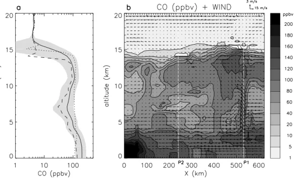
Fig. 5.Simulation results on 8 February 2001 at 22:00 UT.(a)CO averaged over the Grid 2 domain as a function of altitude (bold line) with logarithm scale in horizontal axis. Individual profiles P1 and P2 are also displayed with a dotted line and a dashed line, respectively. The grey area corresponds to the envelope of the mean CO±its standard deviation. (b)Vertical cross-section of CO (contours) and wind field (arrows) located at−22.9◦latitude. The location of profiles P1 and P2 is also indicated by white lines.
Table 4.Statistical results for CO from MOPITT measurements at 700 hPa for the month of February and from the model results for several dates and times. STD stands for the standard deviation.
MOPITT Model 8 February Model 8 February Model 9 February 2001 at 00:00 UT 2001 at 12:00 UT 2001 at 00:00 UT
Mean (ppbv) 91 90 92 96
STD (ppbv) 14 76 70 67
of CO within the 700–500 hPa layer. The model standard deviation is much larger (∼70 ppbv) than the MOPITT stan-dard deviation (14 ppbv). This can be explained by the fact that MOPITT measurements are averaged over a full month leading to a much smoother field than the model instanta-neous fields and that MOPITT averaging kernels were ap-proximated. Only small differences are found between the model statistics for different dates and times, indicating that the model results for the mean CO in the 700–500 hPa layer do not significantly vary during the simulation period.
In order to analyse the impact of convection on the distri-bution of CO, we will focus hereafter on the Grid 2 results since the convection process is explicitly simulated in Grid 2, meaning that no subgrid scale convection parameterization is used. Figure 5a shows the mean profile of CO on 8 February 2001 at 22:00 UT when the convective activity is strongest. It exhibits fairly large values of CO below 2 km altitude of about 20 ppbv. This is due to the large emissions of CO in the
Fig. 6. (a)Mean of NOxmixing ratio over the Grid 2 domain as a function of altitude and(b)corresponding standard deviation. The solid,
dotted and dashed lines correspond respectively to the reference run at 22:00 UT on 8 February 2001, the reference run at 22:00 UT on 7 February 2001 and the “No LNOx” run at 22:00 UT on 8 February 2001. In horizontal axis, the scale is logarithm.
Fig. 7.Mean ethane mixing ratio over Grid 2 domain as a function of altitude for the reference run(a)on 8 February 2001 at 18:00 UT and
(b)on 8 February 2001 at 22:00 UT (solid line) and on 7 February 2001 at 22:00 UT (dotted line). The grey area corresponds to the envelope of the mean ethane±its standard deviation. In horizontal axis, the scale is logarithm.
of wind together with the CO mixing ratio at−22.9◦ lati-tude (Fig. 5b). This cross-section intercepts both convective and non-convective areas. Within the convective cells, the CO emitted at the surface is rapidly transported to the top of the ascent. At−46.5◦longitude, the P1 profile (dotted line)
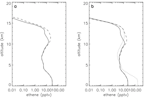
con-Fig. 8. Mean ethene mixing ratio over Grid 2 domain as a function of altitude for the reference run (solid line) and the “No LNOx” run
(dashed line)(a)on 8 February 2001 at 18:00 UT and(b)on 8 February 2001 at 22:00 UT. In (b), the dotted line corresponds to the reference run on 7 February 2001 at 22:00 UT. In horizontal axis, the scale is logarithm.
Fig. 9. Lifetime of ethene in h as a function of altitude for the reference run (solid line) and the “No LNOx” run (dashed line)(a)on 8
February 2001 at 18:00 UT and(b)on 8 February 2001 at 22:00 UT.
vection differs from that within the convective cells. This is shown in Fig. 5a, depicting the profile P2 at−49.3◦ longi-tude (dashed line). In this case, there is a decrease of CO up to 7 km as in the mean CO profile, because there is no updraft to transport CO surface emissions. Above 7 km and below the tropopause, the increase of the CO values is due to the horizontal transport of the large CO amounts from the top
al. (2004) based on a cloud-resolving model. They showed that the tracers emitted in the boundary layer and vertically transported by convection remain in the UT for several days, but only if large-scale forcing is considered in their model. In this case, they found that the large-scale tropospheric ascent partially compensates the net-downward transport of tracers due to the mesoscale subsidence induced by deep convection. The results for CO shown in Fig. 5a were compared with those found by Jonqui`eres and Marenco (1998) from TROPOZ II (TROPOspheric Ozone experiment) observa-tions over Eastern Brazil. The TROPOZ II CO mixing ratios vary from 110 ppbv near the surface to 60–70 ppbv in the 2– 7 km layer while between 7 and 10 km altitude (top of the observations), there was a significant increase of CO up to 120 ppbv at 10 km altitude. Jonqui`eres and Marenco (1998) interpreted this behaviour as a consequence of convective ac-tivity. The model results in the convective area (i.e. Grid 2) show a good consistency with the TROPOZ II measurements since the shape of the model mean CO is similar to the obser-vations with large values near the surface, a decrease between 2 and 7 km and an increase between 7 and 10 km altitude. Moreover, at any level, the observed values fall within the model variability illustrated by the area between the mean± the standard deviation (grey area in Fig. 5a). The mean CO profile plotted in Fig. 5a illustrates the typical behaviour of tracers in the presence of deep convection. This typical pro-file can be divided in 4 layers: layer 1 up to 2 km where the surface emission dominates, layer 2 from 2 to 7 km where the concentration of tracers decreases, layer 3 (or “bulge” layer) from 7 km to the tropopause where there is an en-hancement of tracer mixing ratios related to the effect of up-ward transport by convective ascents only partially compen-sated by a weaker downward transport, and layer 4, above the tropopause, where stratospheric conditions prevail. 5.2 Results for NOx
Figure 6a shows the mean NOx(NO + NO2)profile in Grid 2
at 22:00 UT on 8 February 2001, time of the maximum of convective activity. To study the effect of convection on the NOxvertical distribution, this profile is compared to the
mean NOxprofile at 22:00 UT on 7 February 2001, i.e.
be-fore the convection developed (dotted line in Fig. 6a). The same time of the day is chosen for the two mean profiles since the production and loss of NOx highly depend on the solar
flux. This allows the study of the impact of only the convec-tion process on the NOxvertical distribution, independently
of the solar conditions.
Below∼7 km altitude, the two mean profiles are close and also have similar standard deviations. The differences found around 3 km altitude may be attributed to local dynamical effects. The mean profile at the time of the maximum of con-vection, i.e. 22:00 UT on 8 February 2001, exhibits a large increase of the mean and standard deviation values between 7 km and 17 km altitude compared to the values found 24 h
before, when the convection system has not developed yet. At 22:00 UT on 8 February 2001, the mean NOxmixing ratio
reaches 2 ppbv at∼13 km altitude, while at the same altitude it is only around 0.05 ppbv one day before. To test whether this difference is related to the production of NOx through
lightning originated by the convection, an additional simula-tion was run. This new model run is similar to the reference run described in Sect. 3, but does not include the parameter-ization of the NOxproduction by lightning during the whole
simulation duration. This sensitivity run is called the “No LNOx” run hereafter. In the “No LNOx” run at 22:00 UT on
8 February 2001 (dashed line in Fig. 6), there is no signifi-cant increase of the NOxmixing ratio in the 7–17 km layer
with respect to the reference run at 22:00 UT on 7 February 2001 while large differences are found with respect to the reference run at 22:00 UT on 8 February 2001. The NOx
distribution is mainly determined by the production of NOx
by lightning which provides larger amounts of NOxthan the
vertical transport of emission. Therefore, there is a very large impact of convection in the UT on the NOx mixing ratio,
via the lightning process, leading to a possible effect on the ozone budget.
In the 17–20 km layer, the mean and standard deviation profiles from the reference run and the “No LNOx” run are
very close. This seems to indicate that, on average, there is no vertical transport from the layer below (7–17 km) towards this layer, meaning through the cold point tropopause. This hypothesis was confirmed by the calculation of the NOxflux
through the 17 km level (i.e. approximately the cold point tropopause level) providing weak downward fluxes on aver-age. As for CO, this indicates that there is no dynamical im-pact of the convective cluster on the stratospheric NOxeven
if the convective cells sometimes nearly reach 17 km altitude. 5.3 Results for NMVOCs
The model results for the NMVOCs are displayed in Figs. 7, 8 and 10 showing the mean profile of ethane, ethene and iso-prene in Grid 2. The NMVOC production/loss may largely depend on the solar radiation. Therefore, the NMVOC re-sults are displayed for 7 February 2001 and 8 February 2001 for two different times: 18:00 UT (i.e. during day time) and 22:00 UT (i.e. during sunset). At 18:00 UT the convective system is still growing in intensity while at 22:00 UT the convective activity is at its maximum. The mean profiles at 18:00 UT on 7 February 2001 are not shown since the model is in its spin-up phase at this date/time.
Ethane (C2H6)is a non-methane hydrocarbon. As such,
Fig. 10.Same as Fig. 8 but for isoprene.
Fig. 11.Same as Fig. 9 but for isoprene.
of ethane in the low levels and weaker values in the “bulge layer” compared to 22:00 UT on 8 February 2001. This shows that between these two dates, the ethane emitted at sur-face was lifted by convection in the UT. The profiles for the “No LNOx” run at 18:00 UT and at 22:00 UT have not been
plotted in Fig. 7, because there are only negligible differences compared to the reference run. This indicates that ethane does not depend directly or indirectly on the NOxamount in
the UT. Ethane is a slow reactive compound. Its lifetime is always greater than several tens of days whatever the time of
Fig. 12.Mean HOxmixing ratio over Grid 2 domain as a function
of altitude for the reference run (solid line) and for the “ No LNOx”
run (dashed line) on 8 February 2001 at 18:00 UT.
in Fig. 7a) although the mean values from the model are gen-erally greater (from 0.9 ppbv to 2.5 ppbv) compared to the TROPOZ II observations. This can be explained by the fact that TROPOZ II flights were performed near the coast where emissions were probably lower than in the model Grid 2 box that includes the S˜ao Paulo urban area. In both the model and the TROPOZ II observations, the shape of the vertical distri-bution is similar: first a decrease followed by an increase. The location of the minimum is lower in the observations: about 4 km altitude against 7 km for the model. This may be related to the very high altitude of the 8 February 2001 con-vective ascents that transport surface emissions of ethane to high altitudes.
Figure 8 displays the results for ethene (C2H4). The
com-parison between the reference run at 22:00 UT on 7 February 2001 and on 8 February 2001 shows that, similarly to ethane, convection transports the surface emission up to the UT. In the 7–17 km layer, the ethene lifted by convection is partially depleted in the reference run compared to the “No LNOx”
run, both at 18:00 UT and at 22:00 UT. This means that the NOx produced by lightning have an impact on the ethene
chemistry. Ethene loss is mainly due to reactions with OH that depend largely on the solar radiation. The lifetimes for ethene at 18:00 UT and 22:00 UT are displayed in Fig. 9. At 18:00 UT, the lifetime of ethene is around 5 h, meaning that ethene is significantly depleted during the convective event duration. Moreover, at this time of the day, there are im-portant differences of the lifetime between the reference run and the “No LNOx” run in the 7–17 km layer due to an
in-crease of OH in the reference run and leading to the observed
ethene loss in Fig. 8a. The origin of the OH increase is dis-cussed in Sect. 6. At 22:00 UT, the ethene lifetime is always greater than 24 h because of the rapid decrease of OH at sun-set. Therefore, the loss observed on Fig. 8b between 7 and 15 km altitude is mainly due to the depletion of ethene by OH during the day time before 22:00 UT. In summary, the vertical distribution is of ethene depends on both dynamical effects increasing the ethene content in the UT and chemistry having the contrary effect.
Isoprene (C5H8)is interesting, since it is the most reactive
of the three compounds showed in this section. Figures 10 and 11 displays the mean isoprene profiles and the isoprene lifetimes, respectively. As for ethane and ethene, isoprene is transported to the UT by convective ascents leading to lower values of isoprene in the low levels and higher in the UT. At 18:00 UT, the lifetime of isoprene is around one hour mean-ing that this compound is depleted very rapidly though its re-action with OH at any level. This loss is even more important in the 7–16 km layer when the lightning NOxare taken into
account since there is more OH is this case. At 22:00 UT, the differences between the isoprene lifetime for the reference and for the “No LNOx” runs are important between 7 and
11 km altitude. The lower values of isoprene in the reference run are related the loss that occurred during daytime.
Propene (C3H6)is also an important NMVOC which is
taken into account in the model. The results for propene (not shown) are similar those obtained for ethene and isoprene because its lifetime is between ethene and isoprene.
In the LS (above 17 km), there are no significant changes of all the NMVOC contents even if the cloud top of several of the simulated convective cells nearly reach 17 km altitude. As for CO and NOx, there is no penetration of any of the
simulated convective cells through the isentropic barrier that could lead to troposphere-to-stratosphere transport.
6 Results for HOxand its precursors
The distribution of HOx(OH+HO2)in the atmosphere is of
major importance in the ozone budget since the ozone precur-sors are oxidized through reactions with HOxto form ozone.
Figure 12 represents the mean profiles for HOxat 18:00 UT
on 8 February 2001 for the reference and the “No LNOx”
runs. The 22:00 UT profile is not shown since this is the sun set time corresponding to a rapid decrease of HOxmixing
ra-tios. The HOxmixing ratio for the “No LNOx” run is nearly
constant between 10 and 13.5 km altitude. This is related to the vertical transport by convection of the HOx precursors
as illustrated in Fig. 13 showing a bulge mainly for organic hydroperoxides (noted ROOH) and formaldehyde (HCHO) in the UT. This result is consistent with the model results obtained by DeCaria et al. (2005) within the anvil of a mid-latitude convective system. Another important HOx
Fig. 13.Same as Fig. 12 but for(a)H2O2,(b)organic hydroperoxides (ROOH) and(c)formaldehyde.
increased by 12% at maximum in the UT during the convec-tive period favouring the HOxproduction.
As illustrated in Figs. 12 and 13, there is a significant im-pact of the lightning NOxon HOx and its precursors. The
HOxmean profiles for the two runs are similar except in the
10–16 km altitude range where there is an important decrease of the reference run compared to the “No LNOx” run. This
result is consistent with the mean HOxprofile calculated by
DeCaria et al. (2005). In their case, this decrease was associ-ated to a decrease of both HO2and OH while in the present
study the model simulates on average a decrease of HO2but
an increase of OH. The mechanism responsible for the HO2
decrease is similar in both studies: HO2 reactions with NO
and NO2. For OH, its production/loss depends on the relative
quantity of NOxand VOCs (Volatile Organic Compound). In
both simulations, VOC mixing ratios are high in the UT be-cause of the convective uplift of the surface emissions and consecutive outflow. For the reference run, NOxmixing
ra-tio is very high in the UT mainly where lightning is trig-gered. This leads to two types of mechanisms (Chapter 16 in Finlayson-Pitts and Pitts, 2000):
1. in very localized places where lightning NOx are
pro-duced, the ratio of VOC versus NOxis small enough to
lead to OH depletion forming HNO3.
2. in other places in the vicinity of convective updrafts, a detailed analysis shows that the ratio of VOC versus NOxis large enough to lead to OH production.
On average, this is mechanism 2 that dominates in our sim-ulation leading to a mean increase of OH while in DeCaria et al. (2005) this is mechanism 1. This difference can be ex-plained by different VOC emissions since the geographical
regions considered are very different in the two studies. As in the present study, Wang and Prinn (2000) found an increase of OH during the daytime when NOxare produced by
light-ning from 2-D simulations of a cloud resolving model includ-ing chemistry. Usinclud-ing a global modellinclud-ing approach, Labrador et al. (2004) and Jourdain (2003) obtained similar results on average.
As shown in Figs. 13a and b, lightning NOxtends to
de-plete organic hydroperoxydes and H2O2. This result is in
agreement with DeCaria et al. (2005). The mean formalde-hyde mixing ratio is enhanced in the 9–15 km layer by the increase of NOxby lightning. This is related to the fact that
formaldehyde is formed and depleted at the same time by a complex chain of reactions. In fine, the loss term is of lesser importance, particularly at night time.
In the LS, there is no impact of convection on HOxand its
precursors since the simulated convection cells do not cross the isentropic barrier at the tropopause. This result is similar to that found for the ozone precursors.
7 Summary and conclusion
a severe and very deep convective event that caused flooding in the town of Bauru during the late afternoon of 8 February 2001.
The ERA-40 global analysis is used to initialise the model meteorological fields. For chemical species, MOCAGE global outputs are used. The model is run for two nested grids. The fine grid is focussed on the convective event area with a resolution of 4 km that allows the simulation of con-vection without using a sub-grid scale concon-vection parameter-ization. Meteorological model fields were compared with the near-surface measurements of temperature, wind and relative humidity, as well as with the Bauru radar observations. The simulation provides results in fairly good agreement with these measurements.
Concerning the chemistry results, only the ozone precur-sors, HOxand its precursors are studied in the present paper.
The study of the ozone distribution and budget done in the light of the present analysis is presented in the Part II of this series of papers. Two chemistry simulations were performed. The reference run includes the parameterization of produc-tion of NOxby lightning occurring in convective cells. The
“No LNOx” run does not make use of this parameterisation.
The simulated CO field for the reference run show a good agreement with MOPITT CO measurements for the month of February 2001 at 700 hPa. The model also shows a good agreement with TROPOZ II measurements of CO. CO is a passive tracer at the time scale of the simulation duration. In the convective area, its spatial distribution is closely linked to the dynamics of the convective system with a rapid uplift-ing of surface emissions by the updrafts and then with hori-zontal transport by the outflow at the top of convective cells. The effect of subsidence linked to convection is not strong enough to compensate the upward transport. This leads to larger amounts of CO in the 10–14 km layer. These dynam-ical effects of convection on CO are consistent with previ-ous studies (Wang and Prinn, 2000; Tulet et al., 2002; Salz-mann et al., 2004). Large quantities of NOx, of up to 2 ppbv,
are found in the mid and upper troposphere. These NOxare
produced by lightning associated with the intense convective activity. The surface emissions of NMVOCs (ozone precur-sors) and HOxprecursors are also transported by convection
to the UT. One of the original results of this study is that the production of lightning NOxin the UT leads to a significant
loss of the most reactive NMVOCs (isoprene, propene and ethene) via reactions with OH that is increased on average. This loss and the modification of the HOxbudget influence
the ozone production in the UT as discussed in part II of this series of papers. Lightning NOx tend to deplete HO2 and
HOx precursors except formaldehyde that is enhanced. At
the time of the maximum of convection (22:00 UT, i.e. 19 h local time), the chemical processes become less important since HOxmixing ratio in the troposphere is weaker during
sunset. Another important result is that there is no modifica-tion of the mean ozone precursor contents in the LS for this extreme convective event. Even at the location of the highest
simulated convective cells of the cluster, there is no upward transport through the tropopause isentropic barrier.
The aim of this series of papers is to analyse the impact of convection on the UTLS air composition. For this purpose, the study is done at the scale of the convective event, leading to the use of a fine resolution in the simulation. Therefore, only the local impact is studied at the time scale of the con-vective event (∼12 h). The evolution of ozone and ozone precursors in the tropical UTLS on longer time scales will be the subject of a future study.
To assess the quality of the simulation results, we have used the available chemical observations and data from the literature. Unfortunately, they are not sufficient to validate the model outputs. Therefore, the conclusions of the present paper need to be confirmed by field cam-paigns. This will be possible using the data from the coor-dinated HIBISCUS/TroCCiNOx/TroCCiBras field campaign
that took place in Brazil in February and March 2004. The results of the HIBISCUS/TroCCiNOx/TroCCiBras campaign
will help evaluating the parameterization of production of NOx by ligthning. As already pointed out by Labrador et
al. (2004), this issue is important since it influences largely the NOxbudget, and consequently the budget of NMVOCs,
in the upper troposphere when tropical convection is active. Acknowledgements. This modelling study is supported by funds from the 5t h PCRD (HIBISCUS project) and the French Centre National de le Recherche Scientifique (Programme National de Chimie Atmosph´erique). One of the authors, E. D. Rivi`ere was financially supported in this work by the HIBISCUS European project. This work makes use of the RAMS model, which was developed under the support of the National Science Foundation (NSF) and the Army Research Office (ARO). Computer resources were provided by CINES (Centre Informatique National de l’Enseignement Sup´erieur), project pce2227. The authors thank V.-H Peuch from M´et´eo France for providing the MOCAGE fields that were used to initialise the chemistry model. We also acknowl-edge the MOPITT team at the National Center for Atmospheric Research (Boulder, CO USA) and J.-L. Atti´e for giving the CO gridded data from MOPITT measurements. We thank G. Foret from LaMP for helping with the use of the chemistry model, as well as INMET (Insituto Nacional de Meteorologia, Brazil) for providing surface observations. One of the authors, S. Freitas was financially supported by Fundac¸˜ao de Amparo `a Pesquisa do Estado de S˜ao Paulo (# 01/050125-4). Finally, we thank the referees for their helpful suggestions that improved the quality of the paper.
Edited by: M. G. Lawrence
References
Aumont, B., Jaecker-Voirol,A., Martin, B., and Toupance, G.: Tests of some reduction hypotheses made in photochemical mecha-nisms, Atmos. Env., 30, 2061–2077, 1996.
Barth, M. C., Stuart, A. L., and Skamarock, W. C.: Numerical sim-ulations of the 10 July 1996, Sratospheric-tropospheric experi-ment: radiation, aerosols and ozone (STERAO)– Deep convec-tion experiment storm, redistribuconvec-tion of soluble tracers, J. Geo-phys. Res., 106(D12), 12 381–12 400, 2001.
Barth, M. C., Sillman, S., Hudman, R., Jacobson, M. Z., Kim, C.-H., Monod, A., and Liang, J.: Summary of the cloud chemistry modelling intercomparison, Photochemical box model simulation, J. Geophys. Res., 108(D7), 4214, doi:10.1029/2002JD002673, 2003.
Boissard, C., Bonsang, B., Kanakidou, M., and Lambert, G.: TROPOZ II: Global distributions and budgets of methane and light hydrocarbons, J. Atmos. Chem., 25, 115–148, 1996. Cai, X.-M. and Steyn, D. G.: Modelling study of sea breezes in
a complex coastal environment, Atmos. Env., 34, 2873–2885, 2000.
Cathala, M.-L., Pailleux, J., and Peuch, V.-H.: Improving global simulations of UTLS ozone with assimilation of MOZAIC data, Tellus, 55B, 1–10, 2003.
Clark, T. L. and Farley, R. D.: Severe downslope windstorm cal-culations in two and three spatial dimensions using the anelastic interactive grid nesting, A possible mecanism for gustiness, J. Atmos. Sci., 41, 329–350, 1984.
Clark, T. L. and Hall, W. D.: Multi-domain simulations of the time dependent Navier-Stokes equations: Benchmark error analyis of some nesting procedures, J. Comput. Phys., 92, 456–481, 1991. Cotton, W. R., Pielke Sr., R. A., Walko, R. L., Liston, G. E.,
Tremback, C. J., Jiang, H., McAnelly, R. L., Harrington, J.-Y., Nicholls, M. E., Carrio, G. G., and McFadden, J. P.: RAMS 2001: Current status and future directions, Meteorol. Atmos. Phys., 82, 5–29, DOI 10.1007/s00703-001-0584-9, 2003. DeCaria, A. J., Pickering, K. E., Stenchikov, G. L. and Ott,
L. E.: Lightning-generated NOx and its impact on
tropo-spheric ozone production: A three-dimensional modelling study of a Stratosphere-troposphere experiment, radiation, aerosols and ozone (STERAO-A) thurderstorm, J. Geophys. Res.,110, D14303, doi:10.1029/2004JD005556, 2005.
Deeter, M. N., Emmons, L. K., Francis, G. L., Edwards, D. P., Gille, J. C., Warner, J. X., Khattatov, B., Ziskin, D., Lamarque, J.-F., Ho, S.-P., Atti´e, J.-L., Packman, D., Chen, J., Mao, D., and Drummond, J. R.: Operational carbon moNOxide retrieval
algo-rithm and selected results for the MOPITT instrument, J. Geo-phys. Res., 108(D14), 4399, doi:10.1029/2002JD003186, 2003. Deeter, M. N., Emmons, L. K., Edwards, D. P., and Gille, J.
C.: Vertical resolution and information content of CO pro-files retrieved by MOPITT, Geophys. Res. Letters, 31, L15112, doi:10.1029/2004GL020235, 2004.
Dickerson, R. R., Huffman, G. J., Luke, W. T., Nunnermacker, L. J., Pickering, K. E., Leslie, A. C. D., Lindsey, C. G., Slinn, W. G. N., Kelly, T. J., Daum, P. H., Delany, A. C., Greenberg, J. P., Zimmerman, P. R., Boatman, J. F., Ray, J. D., and Stedman, D. H.: Thunderstorms: an important mechanism in the transport of air pollutants, Science, 235, 460–465, 1987.
Finlayson-Pitts, B. J., and Pitts, Jr J. N. : Chemistry of the up-per and lower atmosphere: theory, exup-periments and applications, Academic Press, San Diego, 2000.
Fishman, J., Hoell Jr, J. M., Bendura, R. D., McNeal Jr, R. J., and Kirchoff, V. W. J. H.: The NASA GTE TRACE-A experiment (September–October, 1992): Overview, J. Geophys. Res., 104, 23 865–23 880, 1996.
Freitas, S., Longo, K., Silva Dias, M., Silva Dias, P., Chatfield, R., Prins, E., Artaxo, P., Grell, G., and Recuero, F.: Monitoring the transport of biomass burning emissions in South America, Environmental Fluid Mechanics, Kluwer Academic Publishers, 5, 135–167, 2005.
Gr´egoire, P. J., Chaumerliac, N., and Nickerson, E. C.: Impact of cloud dynamics on tropospheric chemistry, advances in modeling the interaction between microphysical and chemical processes, J. Atmos. Chem., 18, 247–266, 1994.
Grell, G. A.: Prognostic evaluation of assumptions used by cumulus parameterization, Mon. Wea. Rev., 121, 764–787, 1993. Grell, G. A. and Devenyi, D.: A generalized approach to
parameterizing convection combining ensemble and data as-similation techniques, Geophys. Res. Letters, 29, 1693, doi:10.1029/2002GL015311, 2002.
Held, G. and Nachtigall, L. F.: Flood producing storms in Bauru during February 2001, in Proc XII Congresso Brasileiro de Me-teorologia, SBMET, Foz de Iguac¸u, 3155–3163, 2002.
Hesstvedt, E., Hov, O., and Isaksen, I. S.: Quasi-steady state ap-proximations in air pollution modeling: comparison of two nu-merical schemes for oxidant prediction, Int. J. Chem. Kin., 10, 971, 1978.
Holton, J. R., Haynes, P. H., McIntyre, M. E., Douglass, A. R., Rood, R. B., and Pfister, L.: Stratosphere-Troposphere exchange, Rev. Geophys, 33, 403–439, 1995.
Jonqui`eres, I. and Marenco, A.: Redistribution by deep convec-tion and long-range transport of CO and CH4 emissions from the Amazon basin, as observed by the airborne campaign TROPOZ II during the wet season, J. Geophys. Res., 103, 19 075–19 091, 1998.
Josse B., Simon, P., and Peuch, V.-H.: Rn-222 global simulations with the multiscale CTM MOCAGE, Tellus, 56, 339–356, 2004. Jourdain, L.: Mod´elisation des oxides d’azote et de l’ozone dans le mod`ele de circulation g´en´erale LMDzT-INCA: rˆole des ´emissions par les ´eclairs et par l’aviation subsonique, PhD The-sis, Universit´e Paris 6, 4 July 2003.
Kirchhoff, V. W. J. H., and Alvala, P. C.: Overview of an aircraft expedition into the Brazilian cerrado for the observation of atmo-spheric trace gases, J. Geophys. Res., 101(D19), 23 973–23 981, 1996.
Labrador, L. J., von Kuhlmann, R., and Lawrence, M.G.: Strong sensitivity of the global mean OH concentration and the tropo-spheric oxidizing efficiency to the source of NOxfrom lightning,
Geophy. Res. Lett., 31, L06102, doi:10.1029/2003GL019229, 2004.
Logan, J. A.: An analysis of ozonesonde data for the troposphere: Recommendations for testing three-dimensional models and de-velopment of a gridded climatology for tropospheric ozone, J. Geophys. Res., 104(D23), 16 151–16 170, 1999.
Madronich, S. and Flocke, S.: The role of solar radiation in atmo-spheric chemistry, in: Handbook of Environmental Chemistry edited by: P. Boule, Springer-Verlag, Heidelberg, 1–26, 1999. Marenco, A., Jonqui`eres, I., Gouget, H., and N´ed´elec, P.:
cam-paigns (STRATOZ/TROPOZ) and Pic du Midi data series, Con-sequences on radiative forcing, Global Environmental Change, edited by: W. C. Wang and I. S. A. Isaksen, NATO ASI Ser., 32, 305–319, 1995.
Mari, C., Jacob, D. J., and Bechtold, P.: Transport and scavenging of soluble gases in a deep convective cloud, J. Geophys. Res., 105(D17), 22 255–22 268, 10.1029/2000JD900211, 2000. Mari, C., Sa¨ut, C., Jacob, D. J., Staudt, A., Avery, M. A., Brune,
W. H., Faloona, I., Heikes, B. G., Sachse, G. W., Sandholm, S. T., Singh, H. B., and Tan, D.: On the relative role of convec-tion, chemistry and transport over the South Pacific Convergence Zone during PEM-Tropics B: A case study, J. Geophys. Res., 107, 8232, doi:10.1029/2001JD001466, 2003.
Peuch V.-H., Amodei, M., Barthet, T., Cathala, M.-L., Josse, B., Michou, M., and Simon, P.: MOCAGE, MOd`ele de Chimie At-mosph´erique `a Grande Echelle, In: Proceedings of M´et´eo-France workshop on atmospheric modelling, December 1999, 33–36, 1999.
Pickering, K. E., Thompson, A. M., Dickerson, R. R., Luke, W. T., McNamara, D. P., Greenberg, J. P., and Zimmerman, P. R.: Model calculations of tropospheric ozone production poten-tial following observed convective events, J. Geophys. Res., 95, 14 049–14 062, 1990.
Pickering, K. E., Yansen Wang, Wei-Kuo Tao, Colin Price and M¨uller, J.-F.: Vertical distributions of lightning NOxfor use in
regional and global chemical transport models, J. Geophys. Res., 103, 31 203–31 216, 1998.
Pielke, R. A., Cotton, W. R., Walko, R. L., Tremback, C.J., Lyons, W. A., Grasso, L. D., Nicholls, M. E., Moran, M. D., Wesley, D. A., Lee, T. J., and Copeland, J. H.: A comprehensive meteoro-logical modeling system – RAMS, Meteorol. Atmos., 49, 69–91, 1992.
Poulet, D., Cautenet, S., and Aumont, B.: Simulation of the chem-ical impact of the bush fires emissions in Central Africa during the EXPRESSO campaign, J. Geophys. Res., In revision, 2004. Price, C., Penner, J., and Prather, M.: NOxfrom lightning, 1, Global
distribution based on lightning physics, , J. Geophys. Res., 102, 5929–5941, 1997.
Pundt, I., Pommereau, J.-P., Chipperfield, M. P., Van Roozendael, M., and Goutail, F.: Climatology of the stratospheric BrO ver-tical distribution by balloon-borne UV-Visible spectrometry, J. Geophys. Res., 107 (D24), doi:10.1029/2002JD002230, 2002. Rivi`ere, E. D., Mar´ecal., V., Larsen, N. and Cautenet, S.: Modelling
study of the impact of deep convection on the UTLS air composi-tion, Part 2: Ozone budget in the TTL, Atmos. Chem. and Phys., acp-2005-0110, 2006.
Salzmann, M., Lawrence, M. G., Phillips, V. T. J., and Donner, L. J.: Modelling tracer transport by a cumulus ensemble, lateral bound-ary conditions and large-scale ascent, Atmos. Chem. Phys., 4, 1797–1811, 2004.
Taghavi, M., Cautenet, S. and Foret, G.: Simulation of ozone pro-duction in a complex circulation region using nested grids, At-mos. Chem. Phys., 4, 825–838, 2004.
Thompson, M. A., et al.: Southern hemisphere additional ozoneson-des (SHADOZ) 1998–2000 tropical ozone climatology 2, Tro-pospheric variability and the zonal wave-one, J. Geophys. Res., 108(D2), 8241, doi:1029/2002JD002241, 2003.
Thorntorn, D. C., Bandy, A. R., Blomquist, B. W., Bradshaw, J. D., and Blake, D. R.: Vertical transport of sulfur dioxide and dimethyl sulfide in deep convection and its role in new particle formation, J. Geophys. Res., 102, 28 501–28 509, 1997. Tulet, P., Suhre, K., Mari, C., Solmon, F. and Rosset, R.: Mixing
of boundary layer and upper troposphere ozone during a deep convective event over Western Europe, Atmos. Env., 36, 4491– 4501, 2002.
V¨omel, H., Oltmans, S. J., Johnson, B. J., Hasebe, F., Shiotani, M., Fujiwara, M., Nishi, N., Agama, M., Cornejo, J., Paredes, F., and Enriquez, H.: Balloon-borne observations of water vapor and ozone in the tropical upper troposphere and lower stratosphere, J. Geophys. Res., 107(D14), doi:10.1029/2001JD000707, 2002. Walko, R. L., Tremback, C. J., Pielke, R.A., and Cotton, W. R.:
An interactive nesting algorithm for stretched grids and variable nesting ratios, J. Appl. Meteorol., 34, 994–999, 1995a.
Walko, R. L., Cotton, W. R., Meyers, M. P. and Harrington, J. Y.: New RAMS cloud microphysics parameterization, Part I: the single-moment scheme, 38, 29–62, 1995b.
Wang, Y., Tao, W. K., Pickering, K. E., Thompson, A. M., Kain, J. S., Adler, R. F., Simpson, J., Keehn, P. R., and Lai, G. S.: Mesoscale model simulations of TRACE A and Preliminary Re-gional Experiment for Strom-scale Operational and Reasearch Meteorology convective systems and associated tracer transport, J. Geophys. Res., 101(D19), 24 013–24 027, 1996.
Wang, C. and Prinn, R. G.: On the roles of deep convective clouds in tropospheric chemistry, J. Geophys. Res., 105, 22 269-22 297, 2000.
Willmott, C. J.: On the validation of models, Physical Geography 2, 168–194, 1981.