UNIVERSIDADE FEDERAL DE MINAS GERAIS
HUDSON FERNANDES GOLINO
Modelos Co ple os de P edição Apli ados a Edu ação
Modelos Co ple os de P edição Apli ados a Edu ação
Belo Horizonte
Tese em formato de compilação de artigos apresentada à Universidade Federal de Minas Gerais, como parte dos requisitos para obtenção do grau de Doutor em Neurociências, pelo Programa de Pós-Graduação em Neurociências.
043 Golino, Hudson Fernandes.
Modelos complexos de predição aplicados na educação [manuscrito] /
Hudson Fernandes Golino. – 2015.
127 f. : il. ; 29,5 cm.
Orientador: Cristiano Mauro Assis Gomes.
Tese (doutorado) – Universidade Federal de Minas Gerais, Instituto de
Ciências Biológicas.
1. Aprendizado do computador - Teses. 2. Educação - Teses. 3. Rendimento
escolar - Previsão - Teses. 4. Desempenho - Teses. 5. Neurociências – Teses. I.
Table 1: Usual techniques for assessing the relationship between academic achievement and psychological/educational constructs and its basic assumptions ... 70
Ta le : Fit, elia ilit , odel used a d sa ple size pe test used ……….…
Table 3: Effect sizes, confidence intervals, variance, significance and common language
effect size ……….
Ta le : P edi ti e pe fo a e a hi e lea i g odel ………..
Ta le : Result of the Ma as uilo’s P o edu e ………
Figu e : E a ple of TDRI’s ite f o the fi st de elop e tal stage assessed ………
Figu e : The o elatio at i …...
Figure 3: Single tree grown using the tree package ………
Figure 4: Mean de ease of Gi i I de i the aggi g odel ……….
Figu e : Baggi g’s out-of-bag error (red), high achievement prediction error (green) and
lo a hie e e t p edi tio e o lue ………..
Figure 6: Mean decrease of the Gi i i de i the a do fo est odel ……….
Figu e : Ra do fo est’s out-of-bag error (red), high achievement prediction error
g ee a d lo a hie e e t p edi tio e o lue ………
Figure 8: Mean decrease of the Gini index i the oosti g odel ………….……….
Ta le : Tests, effe t sizes a d o o la guage effe t size CLES ………. 2053
Figure 1: A classification tree from Golino and Gomes ………
Figu e : E a ple of TDRI’s ite f o the fi st de elop e tal stage ……….
Figure 3: Score means and its 95% confidence intervals for each test, by class (high vs. lo a ade i a hie e e t ……….
(mtry), total accuracy, sensitivity, specificity, proportion of misplaced cases (PMC) and mean clustering coefficients for the entire sample, for the target class only and for the non-target class onl ……….………... 2089
Table 2: Correlation between sample size (N), number of trees (ntree), number of predictors (mtry), total accuracy, sensitivity, specificity, proportion of misplaced cases (PMC) and mean clustering coefficients for the entire sample, for the target class only and for the non-ta get lass o l ………..………. 2095
Figure 1: Multisi e sio al s ale plot of the east a e ’s a do fo est p o i it
matrix………
Figure 2: Weighted et o k ep ese tatio of the east a e ’s a do fo est
proximity matrix………
Figure 3: Density distribution of three weighted clustering coefficients (Zhang, Onnela and Barrat) of the malignant class (blue) and the benign class (red), from models 1 to
……….
Figure 4: Multidi e sio al s ale plots of the edi al stude ts’ a do fo est p o i it
matrix………..
Figure 5: Weighted et o k ep ese tatio of the edi al stude ts’ a do fo est
proximity matrix………
Figure 6; Density distribution of three weighted clustering coefficients (Zhang, Onnela and Barrat) of the low achievement class (blue) and the high achievement class (red),
from models 1 to 4………..
Table 2: Kruskal-Wallis Multiple Comparison for different number of p edi to s…………
Table 3: Kruskal-Wallis Multiple Comparison for different number of trees and for the not
imputed dataset (INFIT)……….
Table 4: Va ia ilit of the i fit’s edia , fo ea h u e of p edi to s……… 16
Table 5: Kruskal-Wallis Multiple Comparison for different number of predictors and for
the not imputed dataset (INFIT)……….
Table 6: Kruskal-Wallis Multiple Comparison for different number of trees and for the not imputed dataset ite ’s diffi ult edia ………..…
Table 7: Kruskal-Wallis Multiple Comparison for different number of predictors and for the ot i puted dataset ite ’s diffi ult edia ………
Figure 1: Partitioning of 2-dimensional feature space into four non-overlapping regions
R1, R2, R3 and R4………
Figure 2: Classification Tree………
Figure 3: Inductive Reasoning Developmental Test item example (from the lowest
difficulty level)……….
Figure 4: Median imputation error by experimental condition………..
Figure 5: Person-item map from the not-imputed dataset………..,
Figure 6: Median Infit MSQ by experimental condition. The dark gray line represents the median infit of the not imputed dataset, and the gray rectangle its 95% confidence
interval………..
Figure 7. Median item difficulty by experimental condition. The dark gray line represents the median difficulty of items from the not imputed dataset, and the gray rectangle its
Table 2: Example of the difference between generative and discriminative models towards the probability estimation………..
Table 3: T ee splits a d it’s poste io p o a ilit ………..
Table 4: Variable importance from the Naïve Bayes classifier (or risk factors) ………..
Table 5: Protective factors of academic drop-out……….
Figure 1: Partitioning of 2-dimensional feature space into four non-overlapping regions
R1, R2, R3 and R4………
Figure 2: Classifi atio T ee………..…….
Figure 3: Effect of tree size (number of terminal nodes) in the deviance index, estimated using a 10-fold cross validation of the training set………..
Figure 4: Classification tree with four terminal nodes, constructed after pruning the first
tree………..
Figure 5: ROC curve of the tree classifier and its 95% confidence interval (blue)………….
Figure 6: ROC curve of the Naïve Bayes classifier and its 95% confidence interval (blue). ……….
Figure 7: Comparing the AUC from the learning tree and from the Naïve Bayes
artigo é apresentado os modelos de classification and regression trees, bagging, random
forest e boosting. Esses modelos são empregados para montar um sistema preditivo de
rendimento acadêmico de alunos do ensino superior de uma faculdade particular, tendo uma série de avaliações cognitivas como preditores. Já o segundo artigo emprega o modelo de random forest para predizer o desempenho escolar de alunos do primeiro ano do ensino médio da rede pública. Uma vez mais, um conjunto de avaliações cognitivas foram utilizadas. Já no terceiro artigo, apresentamos uma nova forma de visualizar a qualidade de predições realizadas utilizando a técnica de random forest. Essa nova técnica de visualização transforma informações estatísticas em um gráfico de redes, que possibilita o emprego de um conjunto de indicadores sobre a qualidade da predição, além dos usualmente empregados. No quarto artigo, apresentamos a técnica de random forest como uma nova forma de realizar imputação de dados faltantes. Investigamos o impacto da imputação no ajuste de itens de um teste cognitivo ao modelo dicotômico de Rasch, assim como na dificuldade estimada dos itens. No quinto e último artigo, comparamos o modelo de classification trees com o modelo Naive Bayes na predição de evasão acadêmica de alunos de uma faculdade pública estadual, tendo como preditores variáveis socioeconômicas. Esses artigos introduzem um conjunto de métodos quantitativos que pode auxiliar na resolução de problemas na área da educação, assim como podem levar a novas descobertas, não possibilitadas por meio de métodos usuais.
ABSTRACT
investigação acerca das coisas do mundo (e principalmente a não acreditar em nada, e a desconfiar de tudo).
Agradecimentos
Agradeço infinitamente aos meus pais, Arnaldo e Dinah, que abriram mão de tantas coisas para que eu pudesse estudar e me dedicar à carreira que decidi seguir.
Agradeço imensamente ao meu orientador, Prof. Cristiano Mauro Assis Gomes, por todos os anos de trabalho duro e de grande aprendizado.
Agradeço à minha esposa, Mariana, por todo o amor, carinho e incentivo, tão importantes para minha vida pessoal e profissional.
Agradeço à todos os pesquisadores cujos trabalhos influenciaram direta ou indiretamente os meus projetos. A genialidade da maioria deles ensina não apenas a área ao qual dedicaram suas vidas, mas sobretudo que a ciência só faz sentido se o caminho for o da humildade perante as coisas. Felizmente, minha experiência mostra que a genialidade e a humildade são diretamente proporcionais.
No ano de 2007 iniciei minhas atividades como aluno de iniciação científica sob orientação do Professor Cristiano Mauro Assis Gomes. Naquele período havia um projeto grande em andamento sobre mapeamento da arquitetura cognitiva, utilizando um conjunto de instrumentos de avaliação construídos para serem utilizados nessa pesquisa. Parte dos trabalhos envolvia avaliar um número grande de alunos da educação básica, do sexto ano à terceira série do ensino médio. Após a finalização da coleta dos dados, tivemos que dedicar um vasto tempo na elaboração de relatórios para os alunos, seus pais e para os diretores do colégio. Apesar de perceberem a importância da pesquisa e de gostarem de ver os relatórios de desempenho dos estudantes, a equipe do colégio não havia ficado plenamente satisfeita com a devolutiva dos resultados da pesquisa. Uma das reações mais comuns por parte da equipe do colégio dizia respeito ao que eles poderiam fazer com aqueles resultados. Em outras palavras, pareciam querer saber o que
concretamente poderiam fazer tendo os resultados da pesquisa, e do desempenho dos
alunos, em mãos.
Nos anos posteriores a 2007, continuamos com uma série de projetos que, invariavelmente, envolviam a coleta de dados em escolas ou faculdades. Em absolutamente todas as instituições onde nossos trabalhos foram desenvolvidos, o corpo de diretores, ou de coordenadores, eram monotemáticos. Queriam saber o que poderiam fazer com o resultado do desempenho dos estudantes em uma série de avaliações cognitivas. Explicávamos, de forma sucinta, os modelos teóricos de desenvolvimento da cognição, que serviam de fundamentação para os instrumentos utilizados, e em como eles poderiam ser úteis na condução da política educacional das instituições. Não importa a quantidade de reuniões que pudéssemos fazer, nem os artigos, livros e apresentações que enviávamos para esses profissionais. Simplesmente
ada pa e ia esta de t o do o ju to de ações o etas ue esses p ofissio ais
parecia querer.
Já no ano de 2012, após uma série de experiências fundamentalmente semelhantes às descritas acima, tivemos uma ideia. Poderíamos utilizar o desempenho dos estudantes nas avaliações cognitivas realizadas para construir sistemas de predição do desempenho dos mesmos no colégio ou na faculdade. Com isso, após a condução das atividades de pesquisa, poderíamos apresentar um resultado que possibilitasse ao corpo de diretores incorporar, de forma concreta, as nossas pesquisas em suas atividades institucionais. Além de melhorar o tipo de devolutiva realizada em nossas pesquisas, estaríamos contribuindo de forma significativa com a política educacional dessas instituições. Afinal de contas, ter em mãos uma forma de prever o desempenho acadêmica dos alunos, baseado em avaliações cognitivas, parecia ser uma espécie de
Sa to G aal edu a io al.
utilizadas na modelagem de equação estrutural permitem, dentre outras coisas, verificar o percentual de variância explicada por cada variável preditiva, além dos seus intervalos de confiança. É uma ferramenta extremamente útil. No entanto, ela mudaria pouco o nosso cenário, uma vez que explicar o resultado de uma modelagem de equação estrutural para um público leigo seria pouco útil. Ademais, essa técnica tem uma série de pressupostos que são relativamente difíceis de serem satisfeitos nesse campo.
Sendo assim, começamos a estudar modelos inovadores de predição, ainda pouco utilizados na área da psicologia cognitiva, educacional e áreas afins (apesar de serem muito utilizadas em outros campos, como na ciência da computação), que além de possibilitar a construção de bons modelos preditivos, fossem relativamente simples de explicar para um público leigo. Uma das primeiras ferramentas que encontramos na literatura foi a chamada Classification and Regression Trees (CART). Essa ferramenta foi desenvolvida por Breiman e seus colaboradores na década de 1980 (Breiman, Friedman, Olshen, & Stone, 1984). Dentre várias vantagens da CART encontra-se o fato de que os modelos de predição desenvolvidos são facilmente explicáveis para profissionais com pouco ou nenhum conhecimento estatístico (Geurts, Irrthum, & Wehenkel, 2009), uma vez que assemelha-se a u a sé ie de eg as do tipo se, e tão . Alé disso, as p edições realizadas utilizando-se CART geralmente levam a acurácias mais elevadas do que técnicas mais tradicionais da estatística, como regressão linear, logística, dentre outras (Geurts, Irrthum, & Wehenkel, 2009). Parecia que havíamos encontrado a ferramenta ideal, pois ela possibilitaria criar modelos preditivos relativamente simples de serem explicados, tinha boa chance de levar a acurácias minimamente aceitáveis para o campo, e ai da esol ia, o o e e os ais a ai o, o p o le a dos p essupostos ha d das técnicas usualmente usadas para realizar predições no campo da psicologia cognitiva e educacional (como a modelagem de equações estruturais). No entanto, como em tudo relacionado à ciência, a CART resolve alguns problemas e cria outros, como o sobreajuste e a variância (que também veremos a seguir). Essas características da CART nos fez seguir em busca de outros modelos que pudessem nos ajudar a criar modelos preditivos para as instituições de ensino.
O segundo artigo utiliza apenas o algoritmo de Random Forest para construir um modelo preditivo de desempenho acadêmico na primeira série do ensino médio de um colégio técnico federal. Uma vez mais, os alunos responderam à uma série de instrumentos de avaliação cognitiva, que entraram como as variáveis preditivas (ou a iá eis i depe de tes . A a iá el depe de te utilizada foi a atego ia ap o ado
a i a da édia ou ep o ado o a o leti o. U a das a a te ísti as do Random Forest
é que ele constitui-se o o u a té i a de ai a p eta , o de dife e te e te da CART não há uma árvore típica de predição, e sim uma assembleia de árvores. Dessa forma, compreender o comportamento do algoritmo de predição, ou quão bem ele desempenha a tarefa de predizer a variável dependente, é bastante útil. Geralmente, o campo de
machine learning baseia-se na utilização de indicadores de qualidade de predição, como
a acurácia total, a sensibilidade e a especificidade. No entanto, é também possível utilizar
té i as g áfi as pa a isualiza a ualidade da p edição ealizada. E é esse caminho
que se insere o terceiro artigo deste trabalho, no qual apresentamos uma nova forma de visualizar a qualidade de uma predição realizada via Random Forest, por meio do emprego de representações gráficas de rede.
Outro problema que geralmente enfrentamos na área da psicologia cognitiva e educacional, principalmente quando utilizamos instrumentos de avaliação de variáveis cognitivas, é a quantidade de dados faltantes. Eles surgem por uma série de motivos, que variam desde não conseguir responder à questão/tarefa/item, até o não querer responder, ou esquecer de dar uma resposta. Alguns modelos de análise de dados, como a família de modelos estatísticos de Rasch, da Teoria de Resposta ao Item, lida adequadamente com dados faltantes. No entanto, outros modelos são seriamente afetados na presença de dados faltantes. Por esse motivo, resolvemos realizar um estudo experimental propondo o algoritmo de Random Forest como uma forma de imputação de dados faltantes. O quarto artigo, portanto, mostra o impacto da imputação realizada
via Random Forest no ajuste dos itens de um teste de raciocínio indutivo ao modelo
dicotômico de Rasch, e no parâmetro de dificuldade.
Por último, tivemos acesso a um conjunto de dados socioeconômicos de uma Universidade Estadual localizada no interior da Bahia, que trazia também a situação dos alunos em seus cursos após cerca de quatro anos do ingresso na referida instituição. Já que estávamos trabalhando com a construção de modelos preditivos na área educacional, utilizando métodos inovadores de Machine Learning, resolvemos criar um modelo que predissesse a evasão acadêmica. Esse trabalho foi desenvolvido durante o meu período de Doutorado Sanduiche, no Instituto de Ciências Nucleares da Universidade Nacional Autônoma do México, que focou em mineração de dados.
ensino (principalmente empregando a CART) ou aplicá-los de forma rápida e eficiente (por meio do chamado model deployment, que é a predição de novos dados baseados em modelos previamente elaborados e validados). Assim, é possível oferecer às instituições de ensino parceiras dos nossos projetos algo concreto, i.e. podemos ensiná-los a interpretar o resultado de avaliações cognitivas em termos da probabilidade do aluno ser aprovado ou reprovado no ano/semestre letivo, ou podemos aplicar as avaliações e entregar um resultado que indica se o aluno tem maior chance de ser aprovado ou reprovado. Além disso, esses trabalhos trazem um conjunto de novas possibilidades para o campo, com modelos que não se limitam, no geral, por pressupostos relativamente difíceis de serem atendidos.
68
Four Machine Learning Methods to Predict Academic Achievement of
College Students: A Comparison Study
[Quatro Métodos de Machine Learning para Predizer o Desempenho Acadêmico de
Estudantes Universitários: Um Estudo Comparativo]
HUDSON F. GOLINO1, & CRISTIANO MAURO A. GOMES2
Abstract
The present study investigates the prediction of academic achievement (high vs. low) through four machine learning models (learning trees, bagging, Random Forest and Boosting) using several psychological and educational tests and scales in the following domains: intelligence, metacognition, basic educational background, learning approaches and basic cognitive processing. The sample was composed by 77 college students (55% woman) enrolled in the 2nd and 3rd year of a private Medical School from the state of Minas Gerais, Brazil. The sample was randomly split into training and testing set for cross validation. In the training set the prediction total accuracy ranged from of 65% (bagging model) to 92.50% (boosting model), while the sensitivity ranged from 57.90% (learning tree) to 90% (boosting model) and the specificity ranged from 66.70% (bagging model) to 95% (boosting model). The difference between the predictive performance of each model in training set and in the testing set varied from -2.60% to 23.10% in terms of the total accuracy, from -5.60% to 27.50% in the sensitivity index and from 0% to 20% in terms of specificity, for the bagging and the boosting models respectively. This result shows that these machine learning models can be used to achieve high accurate predictions of academic achievement, but the difference in the predictive performance from the training set to the test set indicates that some models are more stable than the others in terms of predictive performance (total accuracy, sensitivity and specificity). The advantages of the tree-based machine
1
Faculdade Independente do Nordeste (BR). Universidade Federal de Minas Gerais (BR). E-mail: [email protected].
2
69 learning models in the prediction of academic achievement will be presented and discussed throughout the paper.
Keywords: Higher Education; Machine Learning; academic achievement; prediction.
Introduction
The usual methods employed to assess the relationship between psychological
constructs and academic achievement are correlation coefficients, linear and logistic
regression analysis, ANOVA, MANOVA, structural equation modelling, among other
techniques. Correlation is not used in the prediction process, but provides information
regarding the direction and strength of the relation between psychological and
educational constructs with academic achievement. In spite of being useful, correlation
is not an accurate technique to report if one variable is a good or a bad predictor of
another variable. If two variables present a small or non-statistically significant correlation coefficient, it does not necessarily means that one can’t be used to predict the other.
In spite of the high level of prediction accuracy, the artificial neural network
models do not easily allows the identification of how the predictors are related in the
explanation of the academic outcome. This is one of the main criticisms pointed by
researchers against the application of Machine Learning methods in the prediction of
academic achievement, as pointed by Edelsbrunner and Schneider (2013). However,
their Machine Learning methods, as the learning tree models, can achieve a high level
of prediction accuracy, but also provide more accessible ways to identify the
70
Table 1 – Usual techniques for assessing the relationship between academic achievement and psychological/educational constructs and its basic assumptions.
Technique Main Assumptions D is tr ibut ion R el at ions hi p be tw ee n va ri abl es H om os ce da st ic it y? S ens ibl e t o out li er s? Inde pe nde nc e ? S ens ibl e t o C ol li ne ar it y D em ands a hi gh sa m pl e-to -pr edi ct or r at io? S ens ibl e t o m is si n gne ss ?
Correlation Bivariate
Normal Linear Yes Yes NA NA NA Yes
Simple Linear Regression
Normal Linear Yes Yes Predictors are
independent NA Yes Yes
Multiple
Regression Normal Linear Yes Yes
Predictors are independent/Errors
are independent
Yes Yes Yes
ANOVA Normal Linear Yes Yes Predictors are
independent Yes Yes Yes
MANOVA Normal Linear Yes Yes Predictors are
independent Yes Yes Yes
Logistic Regression
True conditional probabilities are a logistic function of the
independent variables Independent variables are not linear combinations of each other
No Yes Predictors are
independent NA Yes Yes
Structural Equation Modelling Normality of univariate distributions Linear relation between every bivariate comparisons
Yes Yes NA NA Yes Yes
The goal of the present paper is to introduce the basic ideas of four specific
learning tree’s models: single learning trees, bagging, Random Forest and Boosting.
These techniques will be applied to predict academic achievement of college students
(high achievement vs. low achievement) using the result of an intelligence test, a basic
cognitive processing battery, a high school knowledge exam, two metacognitive scales
and one learning approaches’ scale. The tree algorithms do not make any assumption
71 collinearity or independency (Geurts, Irrthum, & Wehenkel, 2009). They also do not
demand a high sample-to-predictor ratio and are more suitable to interaction effects than
the classical techniques pointed before. These techniques can provide insightful
evidences regarding the relationship of educational and psychological tests and scales in
the prediction of academic achievement. They can also lead to improvements in the
predictive accuracy of academic achievement, since they are known as the
state-of-the-art methods in terms of prediction accuracy (Geurts et al., 2009; Flach, 2012).
Presenting New Approaches to Predict Academic Achievement
Machine learning is a relatively new science field composed by a broad class of
computational and statistical methods used to extract a model from a system of
observations or measurements (Geurts et al., 2009; Hastie, Tibshirani, & Friedman,
2009). The extraction of a model from the sole observations can be used to accomplish
different kind of tasks for predictions, inferences, and knowledge discovery (Geurts et
al., 2009; Flach, 2012).
Machine Learning techniques are divided in two main areas that accomplish
different kinds of tasks: unsupervised and supervised learning. In the unsupervised
learning field the goal is to discover, to detect or to learn relationships, structures, trends
or patterns in data. There is a d-vector of observations or measurements of features, , but no previously known outcome, or no associated response (Flach, 2012; James, Witten, Hastie, & Tibshirani, 2013). The features can
be of any kind: nominal, ordinal, interval or ratio.
In the supervised learning field, by its turn, for each observation of the predictor
(or independent variable) , , there is an associated response or outcome .
The vector belongs to the feature space , , and the vector belongs to the
output space , . The task can be a regression or a classification. Regression is
used when the outcome has an interval or ratio nature, and classification is used when
the outcome variable has a categorical nature. When the task is of classification (e.g.
classifying people into a high or low academic achievement group), the goal is to
72 composed by a small and finite set of classes , so that . In
this case the output space is the set of finite classes: . In sum, in the classification
problem a categorical outcome (e.g. high or low academic achievement), is predicted
using a set of features (or predictors, independent variables). In the regression task, the
value of an outcome in interval or ratio scale (for example the Rasch score of an
intelligence test) is predicted using a set of features. The present paper will focus in the
classification task.
From among the classification methods of Machine Learning, the tree based
models are supervised learning techniques of special interest for the education research
field, since it is useful: 1) to discover which variable, or combination of variables, better
predicts a given outcome (e.g. high or low academic achievement); 2) to identify the
cutoff points for each variable that are maximally predictive of the outcome; and 3) to
study the interaction effects of the independent variables that lead to the purest
prediction of the outcome.
A classification tree partitions the feature space into several distinct mutually
exclusive regions (non-overlapping). Each region is fitted with a specific model that
performs the labeling function, designating one of the classes to that particular space.
The class is assigned to the region of the feature space by identifying the majority
class in that region. In order to arrive in a solution that best separates the entire feature
space into more pure nodes (regions), recursive binary partitions is used. A node is
considered pure when 100% of the cases are of the same class, for example, low
academic achievement. A node with 90% of low achievement and 10% of high
achievement students is more “pure” then a node with 50% of each. Recursive binary
partitions work as follows. The feature space is split into two regions using a specific
cutoff from the variable of the feature space that leads to the most purity
configuration. Then, each region of the tree is modeled accordingly to the majority
class. Then one or two original nodes are split into more nodes, using some of the given
predictor variables that provide the best fit possible. This splitting process continues
until the feature space achieves the most purity configuration possible, with regions
or nodes classified with a distinct class. Learning trees have two main basic tuning
73 Stone, 1984): 1) the number of features used in the prediction , and 2) the
complexity of the tree, which is the number of possible terminal nodes .
If more than one predictor is given, then the selection of each variable used to
split the nodes will be given by the variable that splits the feature space into the most
purity configuration. It is important to point that in a classification tree, the first split
indicates the most important variable, or feature, in the prediction. Leek (2013)
synthesizes how the tree algorithm works as follow: 1) iteratively split variables into
groups; 2) split the data where it is maximally predictive; and 3) maximize the amount
of homogeneity in each group.
The quality of the predictions made using single learning trees can verified using
the misclassification error rate and the residual mean deviance (Hastie et al., 2009). In
order to calculate both indexes, we first need to compute the proportion of class in
the node . As pointed before, the class to be assigned to a particular region or node
will be the one with the greater proportion in that node. Mathematically, the proportion
of class in a node of the region , with people is:
The labeling function that will assign a class to a node is: . The
misclassification error is simply the proportion of cases or observations that do not
belong to the class in the region:
and the residual mean deviance is given by the following formula:
74 where is the number of people (or cases/observations) from the class in the
region, is the size of the sample, and is the number of terminal nodes (James et al.,
2013).
Deviance is preferable to misclassification error because is more sensitive to node purity. For example, let’s suppose that two trees (A and B) have 800 observations each, of high and low achievement students (50% in each class). Tree A have two nodes,
being A1 with 300 high and 100 low achievement students, and A2 with 100 high and
300 low achievement students. Tree B also have two nodes: B1 with 200 high and 400
low, and B2 with 200 high and zero low achievement students. The misclassification
error rate for tree A and B are equal (.25). However, tree B produced more pure nodes,
since node B2 is entirely composed by high achievement people, thus it will present a
smaller deviance than tree A. A pseudo R2 for the tree model can also be calculated
using the deviance:
Pseudo R2 = .
Geurts, Irrthum and Wehenkel (2009) argue that learning trees are among the
most popular algorithms of Machine Learning due to three main characteristics:
interpretability, flexibility and ease of use. Interpretability means that the model
constructed to map the feature space into the output space is easy to understand, since it
is a roadmap of if-then rules. James, Witten, Hastie and Tibshirani (2013) points that the
tree models are easier to explain to people than linear regression, since it mirrors more
the human decision-making then other predictive models. Flexibility means that the tree
techniques are applicable to a wide range of problems, handles different kind of
variables (including nominal, ordinal, interval and ratio scales), are non-parametric
techniques and does not make any assumption regarding normality, linearity or
independency (Geurts et al., 2009). Furthermore, it is sensible to the impact of
additional variables to the model, being especially relevant to the study of incremental
validity. It also assesses which variable or combination of them, better predicts a given
75 Finally, the ease of use means that the tree based techniques are computationally simple,
yet powerful.
In spite of the qualities of the learning trees pointed above, the techniques suffer
from two related limitations. The first one is known as the overfitting issue. Since the
feature space is linked to the output space by recursive binary partitions, the tree models
can learn too much from data, modeling it in such a way that may turn out a sample
dependent model. Being sample dependent, in the sense that the partitioning is too
suitable to the data set in hand, it will tend to behave poorly in new data sets. The
second issue is exactly a consequence of the overfitting, and is known as the variance
issue. The predictive error in a training set, a set of features and outputs used to grown a
classification tree for the first time, may be very different from the predictive error in a
new test set. In the presence of overfitting, the errors will present a large variance fr om
the training set to the test set used. Additionally, the classification tree does not have the
same predictive accuracy as other classical Machine Learning approaches (James et al.,
2013). In order to prevent overfitting, the variance issue and also to increase the
prediction accuracy of the classification trees, a strategy named ensemble techniques
can be used.
Ensemble techniques are simply the junction of several trees to perform the
classification task based on the prediction made by every single tree. There are three
main ensemble techniques to classification trees: bagging, Random Forest and boosting.
The first two techniques increases prediction accuracy and decreases variance between
data sets as well as avoid overfitting. The boosting technique, by its turn, only increases
accuracy but can lead to overfitting (James et al., 2013).
Bagging (Breiman, 2001b) is the short hand for bootstrap aggregating, and is a
general procedure for reducing the variance of classification trees (Hastie et al., 2009;
Flach, 2012; James et al., 2013). The procedure generates different bootstraps from
the training set, growing a tree that assign a class to the regions of the feature
space for every . Lastly, the class of regions of each tree is recorded and the
majority vote is taken (Hastie et al., 2009; James et al., 2013). The majority vote is
simply the most commonly occurring class over all trees. As the bagged trees does
not use the entire observations (only a bootstrapped subsample of it, usually 2/3), the
76 the prediction. The out-of-bag error can be computed as a «valid estimate of the test
error for the bagged model, since the response for each observation is predicted using
only the trees that were not fit using that observation» (James et al., 2013, p.323).
Bagged trees have two main basic tuning parameters: 1) the number of features used in
the prediction, , is set as the total number of predictors in the feature space, and 2)
the size of the bootstrap set , which is equal the number of trees to grow.
The second ensemble technique is the Random Forest (Breiman, 2001a). Random
Forest differs from bagging since the first takes a random subsample of the original
data set with replacement to growing the trees, as well as selects a subsample of
the feature space at each node, so that the number of the selected features (variables)
is smaller than the number of total elements of the feature space: . As
points Breiman (2001a), the value of is held constant during the entire procedure
for growing the forest, and usually is set to . By randomly subsampling the
original sample and the predictors, Random Forest improves the bagged tree method by
decorrelating the trees (Hastie et al., 2009). Since it decorrelates the trees grown, it also
decorrelate the errors made by each tree, yielding a more accurate prediction.
And why the decorrelation is important? James et al. (2013) create a scenario to
make this characteristic clear. Let’s follow their interesting argument. Imagine that we
have a very strong predictor in our feature space, together with other moderately strong
predictors. In the bagging procedure, the strong predictor will be in the top split of most
of the trees, since it is the variable that better separates the classes. By consequence,
the bagged trees will be very similar to each other with the same variable in the top
split, making the predictions highly correlated, and thus the errors also highly
correlated. This will not lead to a decrease in the variance if compared to a single tree.
The Random Forest procedure, on the other hand, forces each split to consider only a
subset of the features, opening chances for the other features to do their job. The strong
predictor will be left out of the bag in a number of situations, making the trees very
different from each other. As a result, the resulting trees will present less variance in the
classification error and in the OOB error, leading to a more reliable prediction. Random
77 used in each split, , which is mandatory to be , being generally set
as and 2) the size of the set , which is equal the number of trees to grow.
The last technique to be presented in the current paper is the boosting (Freund &
Schapire, 1997). Boosting is a general adaptive method, and not a traditional ensemble
technique, where each tree is constructed based on the previous tree in order to increase
the prediction accuracy. The boosting method learns from the errors of previous trees,
so unlikely bagging and Random Forest, it can lead to overfitting if the number of trees
grown is too large. Boosting has three main basic tuning parameters: 1) the size of the
set , which is equal the number of trees to grow, 2) the shrinkage parameter , which
is the rate of learning from one tree to another, and 3) the complexity of the tree, which
is the number of possible terminal nodes . James et al. (2013) point that is
usually set to 0.01 or to 0.001, and that the smaller the value of , the highest needs to
be the number of trees , in order to achieve good predictions.
The Machine Learning techniques presented in this paper can be helpful in
discovering which psychological or educational test, or a combination of them, better
predict academic achievement. The learning trees have also a number of advantages over the most traditional prediction models, since they doesn’t make any assumptions regarding normality, linearity or independency of the variables, are non-parametric,
handles different kind of predictors (nominal, ordinal, interval and ratio), are applicable
to a wide range of problems, handles missing values and when combined with ensemble
techniques provide the state-of-the-art results in terms of accuracy (Geurts et al., 2009).
The present paper introduced the basics ideas of the learning trees’ techniques, in
the first two sections above, and now they will be applied to predict the academic
achievement of college students (high achievement vs. low achievement). Finally, the
results of the four methods (single trees, bagging, Random Forest and boosting) will be
78 Methods
Participants
The sample is composed by 77 college students (55% woman) enrolled in the 2nd
and 3rd year of a private Medical School from the state of Minas Gerais, Brasil. The sample was selected randomly, using the faculty’s data set with the student’s achievement recordings. From all the 2nd and 3rd year students we selected 50 random
students with grades above 70% in the last semester, and 50 random students with
grades equal to or below 70%. The random selection of students was made without
replacement. The 100 random students selected to participate in the current study
received a letter explaining the goals of the research, and informing the assessment
schedule (days, time and faculty room). Those who agreed in being part of the study
signed a inform consent, and confirmed they would be present in the schedule days to
answer all the questionnaires and tests. From all the 100 students, only 77 appeared in
the assessment days.
Instruments
The Inductive Reasoning Developmental Test (TDRI) was developed by Gomes
and Golino (2009) and by Golino and Gomes (2012) to assess developmental stages of
reasoning based on Common’s Hierarchical Complexity Model (Commons & Richards,
1984; Commons, 2008; Commons & Pekker, 2008) and on Fischer’s Dynamic Skill
Theory (Fischer, 1980; Fischer & Yan, 2002). This is a pencil-and-paper test composed
by 56 items, with a time limit of 100 minutes. Each item presents five letters or set of
letters, being four with the same rule and one with a different rule. The task is to
identify which letter or set of letters have the different rule.
79 Golino and Gomes (2012) evaluated the structural validity of the TDRI using
responses from 1459 Brazilian people (52.5% women) aged between 5 to 86 years
(M=15.75; SD=12.21). The results showed a good fit to the Rasch model (Infit: M=.96;
SD=.17) with a high separation reliability for items (1.00) and a moderately high for people (.82). The item’s difficulty distribution formed a seven cluster structure with gaps between them, presenting statistically significant differences in the 95% c.i. level
(t-test). The CFA showed an adequate data fit for a model with seven first-order factors
and one general factor [χ2(61)= 8832.594, p=.000; CFI=.96; RMSEA=.059]. The latent
class analysis showed that the best model is the one with seven latent classes
(AIC:263.380; BIC:303.887; Loglik:-111.690). The TDRI test has a self-appraisal scale
attached to each one of the 56 items. In this scale, the participants are asked to appraise
their achievement on the TDRI items, by reporting if he/she passed or failed the item.
The scoring procedure of the TDRI self-appraisal scale works as follows. The
participant receive a score of 1 in two situations: 1) if the participant passed the ith item
and reported that he/she passed the item, and 2) if the participant failed the ith item and
reported that he/she failed the item. On the other hand, the participant receives a score
of 0 if his appraisal does not match his performance on the ith item: 1) he/she passed the
item, but reported that failed it, and 2) he/she failed the item, but reported that passed it.
The Metacognitive Control Test (TCM) was developed by Golino and Gomes
(2013) to assess the ability of people to control intuitive answers to
logical-mathematical tasks. The test is based on Shane Frederick’s Cognitive Reflection Test
(Frederick, 2005), and is composed by 15 items. The structural validity of the test was
assessed by Golino and Gomes (2013) using responses from 908 Brazilian people
(54.8% women) aged between 9 to 86 years (M=27.70, SD=11.90). The results showed
a good fit to the Rasch model (Infit: M=1.00; SD=.13) with a high separation reliability
for items (.99) and a moderately high for people (.81). The TCM also has a
self-appraisal scale attached to each one of its 15 items. The TCM self-self-appraisal scale is
scored exactly as the TDRI self-appraisal scale: an incorrect appraisal receives a score
of 0, and a correct appraisal receives a score of 1.
The Brazilian Learning Approaches Scale (EABAP) is a self-report questionnaire
composed by 17 items, developed by Gomes and colleagues (Gomes, 2010; Gomes,
80 deep learning approaches, and eight items measure surface learning approaches. Each
item has a statement that refers to a student’s behavior while learning. The student
considers how much of the behavior described is present in his life, using a Likert -like
scale ranging from (1) not at all, to (5) entirely present. BLAS presents reliability,
factorial structure validity, predictive validity and incremental validity as good marker
of learning approaches. These psychometrical proprieties are described respectively in
Gomes et al. (2011), Gomes (2010), and Gomes and Golino (2012). In the present
study, the surface learning approach items scale were reverted in order to indicate the
deep learning approach. So, the original scale from 1 (not at all) to 5 (entirely present),
that related to surface learning behaviors, was turned into a 5 (not at all) to 1 (entirely
present) scale of deep learning behaviors. By doing so, we were able to analyze all 17
items using the partial credit Rasch Model.
The Cognitive Processing Battery is a computerized battery developed by
Demetriou, Mouyi and Spanoudis (2008) to investigate structural relations between
different components of the cognitive processing system. The battery has six tests:
Processing Speed (PS), Discrimination (DIS), Perceptual Control (PC), Conceptual
Control (CC), Short-Term Memory (STM), and Working Memory (WM). Golino,
Gomes and Demetriou (2012) translated and adapted the Cognitive Processing Battery
to Brazilian Portuguese. They evaluated 392 Brazilian people (52.3% women) aged
between 6 to 86 years (M= 17.03, SD= 15.25). The Cognitive Processing Battery tests presented a high reliability (Cronbach’s Alpha), ranging from .91 for PC and .99 for the STM items. WM and STM items were analyzed using the dichotomous Rasch Model,
and presented an adequate fit, each one showing an infit meansquare mean of .99
(WM’s SD=.08; STM’s SD=.10). In accordance with earlier studies, the structural
equation modeling of the variables fitted a hierarchical, cascade organization of the
constructs (CFI=.99; GFI=.97; RMSEA=.07), going from basic processing to complex
processing: PS DIS PC CC STM WM.
The High School National Exam (ENEM) is a 180 item educational examination created by Brazilian’s Government to assess high school student’s abilities on school subjects (see http://portal.inep.gov.br/). The ENEM result is now the main student’s
81
The student’s ability estimates on the Inductive Reasoning Developmental Test
(TDRI), on the Metacognitive Control Test (TCM), on the Brazilian Learning
Approaches Scale (EABAP), and on the memory tests of the Cognitive Processing
Battery, were computed using the original data set of each test, using the software
Winsteps (Linacre, 2012). This procedure was followed in order to achieve reliable
estimates, since only 77 medical students answered the tests. The mixture of the original
data set with the Medical School students’ answers didn’t change the reliability or fit to
the models used. A summary of the separation reliability and fit of the items, the
separation reliability of the sample, the statistical model used, and the number of
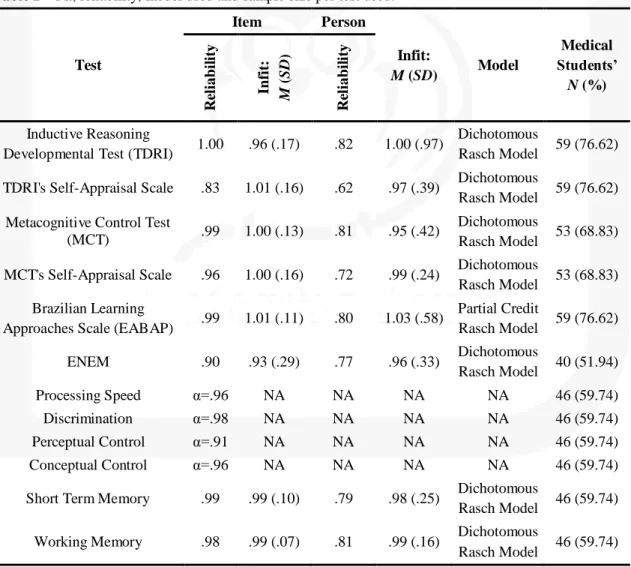
medical students that answered each test is provided in Table 2.
Table 2 – Fit, reliability, model used and sample size per test used.
Test
Item Person
Infit:
M (SD) Model
Medical Students’ N (%) R el iab il it y In fi t: M ( SD ) R el iab il it y Inductive Reasoning
Developmental Test (TDRI) 1.00 .96 (.17) .82 1.00 (.97)
Dichotomous
Rasch Model 59 (76.62)
TDRI's Self-Appraisal Scale .83 1.01 (.16) .62 .97 (.39) Dichotomous
Rasch Model 59 (76.62)
Metacognitive Control Test
(MCT) .99 1.00 (.13) .81 .95 (.42)
Dichotomous
Rasch Model 53 (68.83)
MCT's Self-Appraisal Scale .96 1.00 (.16) .72 .99 (.24) Dichotomous
Rasch Model 53 (68.83) Brazilian Learning
Approaches Scale (EABAP) .99 1.01 (.11) .80 1.03 (.58)
Partial Credit
Rasch Model 59 (76.62)
ENEM .90 .93 (.29) .77 .96 (.33) Dichotomous
Rasch Model 40 (51.94) Processing Speed α=.96 NA NA NA NA 46 (59.74)
Discrimination α=.98 NA NA NA NA 46 (59.74) Perceptual Control α=.91 NA NA NA NA 46 (59.74) Conceptual Control α=.96 NA NA NA NA 46 (59.74)
Short Term Memory .99 .99 (.10) .79 .98 (.25) Dichotomous
Rasch Model 46 (59.74)
Working Memory .98 .99 (.07) .81 .99 (.16) Dichotomous
82 Procedures
After estimating the student’s ability in each test or extracting the mean response time (in the computerized tests: PS, DIS, PC and CC) the Shapiro-Wilk test of
normality was conducted in order to discover which variables presented a normal
distribution. Then, the correlations between the variables were computed using the
heterogeneous correlation function (hector) of the polycor package (Fox, 2010) of the R
statistical software. To verify if there was any statistically significant difference
between the students’ groups (high achievement vs. low achievement) the two-sample T
test was conducted in the normally distributed variables and the Wilcoxon Sum-Rank
test in the non-normal variables, both at the 0.05 significance level. In order to estimate
the effect sizes of the differences the R’s compute.es package (Del Re, 2013) was used.
This package computes the effect sizes, along with their variances, confidence intervals,
p-values and the common language effect size (CLES) indicator using the p-values of
the significance testing. The CLES indicator expresses how much (in %) the score from
one population is greater than the score of the other population if both are randomly
selected (Del Re, 2013).
The sample was randomly split in two sets, training and testing. The training set is
used to grow the trees, to verify the quality of the prediction in an exploratory fashion,
and to adjust the tuning parameters. Each model created using the training set is applied
in the testing set to verify how it performs on a new data set.
The single learning tree technique was applied in the training set having all the
tests plus sex as predictors, using the package tree (Ripley, 2013) of the R software. The
quality of the predictions made in the training set was verified using the
misclassification error rate, the residual mean deviance and the Pseudo R2. The
prediction made in the cross-validation using the test set was assessed using the total
accuracy, the sensitivity and the specificity. Total accuracy is the proportion of
observations correctly classified:
83 where is the number of observations in the testing set. The sensitivity is the rate of
observations correctly classified in a target class, e.g. , over the
number of observations that belong to that class:
Finally, specificity is the rate of correctly classified observations of the non-target
class, e.g. , over the number of observations that belong to
that class:
The bagging and the Random Forest technique were applied using the
randomForest package (Liaw & Wiener, 2012). As the bagging technique is the
aggregation trees using n random subsamples, the randomForest package can be used to
create the bagging classification by setting the number of features (or predictors) equal
the size of the feature set: . In order to verify the quality of the prediction
both in the training (modeling phase) and in the testing set (cross-validation phase), the
total accuracy, the sensitivity and specificity were used. Since the bagging and the
random forest are black box techniques – i.e. there is only a prediction based on
majority vote and no “typical tree” to look at the partitions – to determine which
variable is important in the prediction two importance measures will be used: the mean
decrease of accuracy and the mean decrease of the Gini index. The former indicates
how much in average the accuracy decreases on the out-of-bag samples when a given
variable is excluded from the model (James et al., 2013). The latter indicates «the total
decrease in node impurity that results from splits over that variable, averaged over all
trees» (James et al., 2013, p.335). The Gini Index can be calculated using the formula
84
Finally, in order to verify which model presented the best predictive performance
(accuracy, sensitivity and specificity) the Marascuilo (1966) procedure was used. This
procedure points if the difference between all pairs of proportions is statistically
significant. Two kinds of comparisons were made: difference between sample sets and
differences between models. In the Marascuilo procedure, a test value and a critical
range is computed to all pairwise comparisons. If the test value exceeds the critical
range the difference between the proportions is considered significant at .05 level. A
more deep explanation of the procedure can be found at the NIST/Semantech website
[http://www.itl.nist.gov/div898/handbook/prc/section4/prc474.htm]. The complete
dataset used in the current study (Golino & Gomes, 2014) can be downloaded for free at
http://dx.doi.org/10.6084/m9.figshare.973012.
Results
The only predictors that showed a normal distribution were the EABAP (W=.97,
p=.47), the ENEM exam (W=.97, p=.47), processing speed (W=.95, p=.06) and
perceptual control (W=.95, p=.10). All other variables presented a p-value smaller than
.05. In terms of the difference between the high and the low achievement groups there
was a statistically significant difference at the 95% level in the mean ENEM Rasch
score ( High=1.13, =1.24, Low=-1.08, Low=2.68, t(39)=4.8162, p=.000), in the
median Rasch score of the TDRI ( High=1.45, = 2.23, Low = .59, Low=1.58,
W=609, p=.008), in the median Rasch score of the TCM
( High=1.03, =2.96, Low=-2.22, Low=8.61, W=526, p=.001), in the median Rasch
score of the TDRI’s self-appraisal scale ( High=2.00, =2.67, Low=1.35, Low=1.63,
W=646, p=.001), in the median Rasch score of the TCM’s self-appraisal scale
( High=1.90, =3.25, Low=-1.46, Low=5.20, W=474, p=.000), and in the median
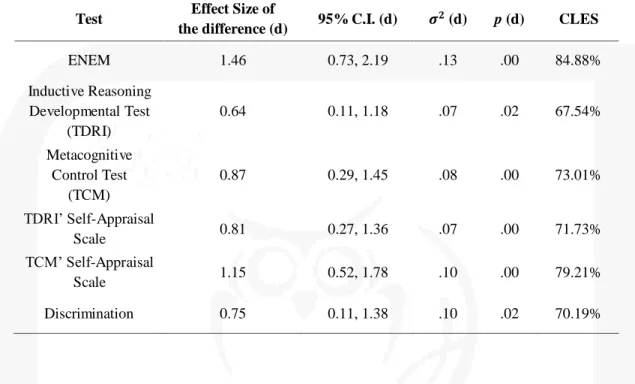
85 The effect sizes, its 95% confidence intervals, variance, significance and common
language effect sizes are described in Table 3.
Table 3 – Effect Sizes, Confidence Intervals, Variance, Significance and Common Language Effect Sizes (CLES).
Test Effect Size of
the difference (d) 95% C.I. (d) (d) p (d) CLES
ENEM 1.46 0.73, 2.19 .13 .00 84.88%
Inductive Reasoning Developmental Test
(TDRI)
0.64 0.11, 1.18 .07 .02 67.54%
Metacognitive Control Test
(TCM)
0.87 0.29, 1.45 .08 .00 73.01%
TDRI’ Self-Appraisal
Scale 0.81 0.27, 1.36 .07 .00 71.73%
TCM’ Self-Appraisal
Scale 1.15 0.52, 1.78 .10 .00 79.21%
Discrimination 0.75 0.11, 1.38 .10 .02 70.19%
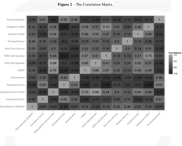
Considering the correlation matrix presented in Figure 2, the only variables with
moderate correlations (greater than .30) with academic grade was the TCM (.54), the
TDRI (.46), the ENEM exam (.49), the TCM Self-Appraisal Scale (.55) and the TDRI
Self-Appraisal Scale (.37). The other variables presented only small correlations with
the academic grade. So, considering the analysis of differences between groups, the size
of the effects and the correlation pattern, it is possible to elect some variables as
favorites for being predictive of the academic achievement. However, as the learning
tree analysis showed, the picture is a little bit different than showed in Table 2 and
Figure 2.
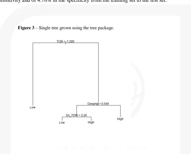
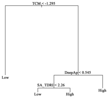
In spite of inputting all the tests plus sex as predictors in the single tree analysis,
the tree package algorithm selected only three of them to construct the tree: the TCM,
the EABAP (in the Figure 3, represented as DeepAp) and the TDRI’ Self-Appraisal
Scale (in the Figure 3, represented as SA_TDRI). These three predictors provided the
best split possible in terms of misclassification error rate (.27), residual mean deviance
86 nodes (Figure 3). The TCM is the top split of the tree, being the most important
predictor, i.e. the one who best separates the observations into two nodes. People with
TCM’ Rasch score lower than -1.29 are classified as being part of the low achievement
class, with a probability of 52.50%.
Figure 2 – The Correlation Matrix.
By its turn, people with TCM’ Rasch score greater than -1.29 and with EABAP’s
Rasch score (DeepAp) greater than 0.54 are classified as being part of the high
achievement class, with a probability of 60%. People are also classified as belonging to
the high achievement class if they present a TCM’ Rasch score greater than -1.29, an
EABAP’s Rasch Score (DeepAp) greater than 0.54, but a TDRI’s Self-Appraisal Rasch
Score greater than 2.26, with a probability of 80%. On the other hand, people are
87 the same profile as the previous one but the TDRI’s Self-Appraisal Rasch score being
less than 2.26. The total accuracy of this tree is 72.50%, with a sensitivity of 57.89%
and a specificity of 85.71%. The tree was applied in the testing set for cross-validation,
and presented a total accuracy of 64.86%, a sensitivity of 43.75% and a specificity of
80.95%. There was a difference of 7.64% in the total accuracy, of 14.14% in the
sensitivity and of 4.76% in the specificity from the training set to the test set.
Figure 3 – Single tree grown using the tree package.
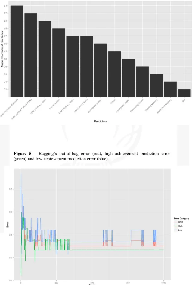
The result of the bagging model with one thousand bootstrapped samples showed
an out-of-bag error rate of .37, a total accuracy of 65%, a sensitivity of 63.16% and a
specificity of 66.67%. Analyzing the mean decrease in the Gini index, the three most
important variables for node purity were, in decreasing order of importance: Deep
Approach (EABAP), TCM, and TDRI Self-Appraisal (Figure 4). The higher the
decrease in the Gini index, the higher the node purity when the variable is used.
Figure 5 shows the high achievement prediction error (green line), out-of-bag
error (red line) and low achievement prediction error (black line) per tree. The errors
88
Figure 4 – Mean decrease of the Gini index in the Bagging Model.
89 The bagging model was applied in the testing set for cross-validation, and
presented a total accuracy of 67.56%, a sensitivity of 68.75% and a specificity of
66.67%. There was a difference of 2.56% in the total accuracy and of 5.59% in the
sensitivity. No difference in the specificity from the training set to the test set was
found.
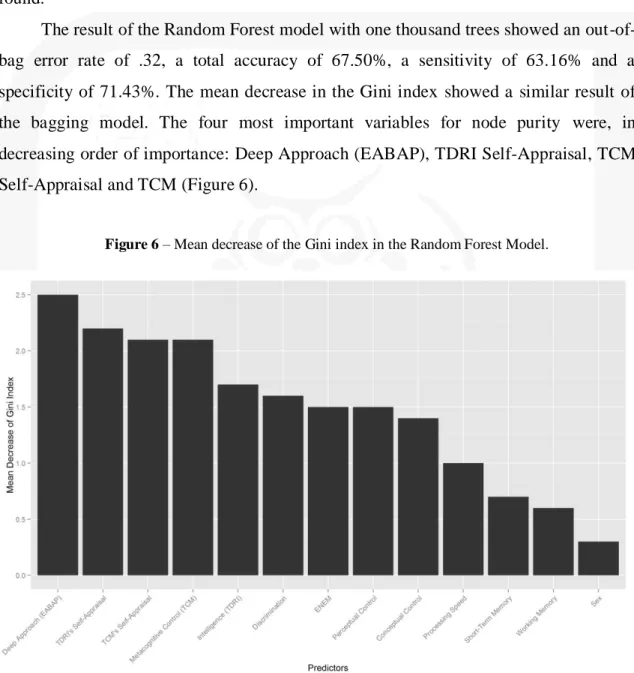
The result of the Random Forest model with one thousand trees showed an
out-of-bag error rate of .32, a total accuracy of 67.50%, a sensitivity of 63.16% and a
specificity of 71.43%. The mean decrease in the Gini index showed a similar result of
the bagging model. The four most important variables for node purity were, in
decreasing order of importance: Deep Approach (EABAP), TDRI Self-Appraisal, TCM
Self-Appraisal and TCM (Figure 6).
Figure 6 – Mean decrease of the Gini index in the Random Forest Model.
The Random Forest model was applied in the testing set for cross-validation, and
presented a total accuracy of 72.97%, a sensitivity of 56.25% and a specificity of
81.71%. There was a difference of 5.47% in the total accuracy, of 6.91% in the
90 Figure 7 shows the high achievement prediction error (green line), out-of-bag
error (red line) and low achievement prediction error (black line) per tree. The errors
became more stable with approximately more than 250 trees.
Figure 7 –Random Forest’s out-of-bag error (red), high achievement prediction error (green) and low achievement prediction error (blue).
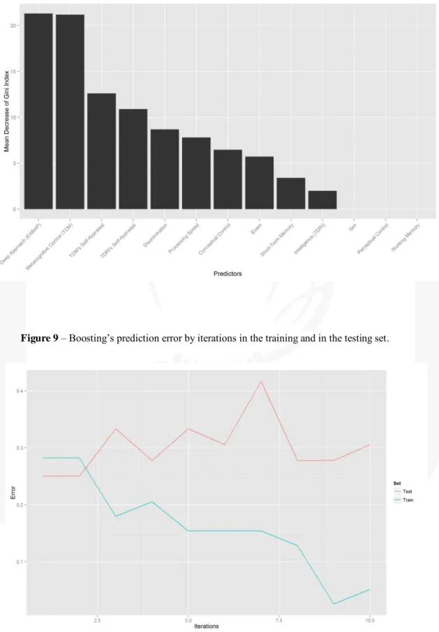
The result of the boosting model with ten trees, shrinkage parameter of 0.001, tree
complexity of two, and setting the minimum number of split to one, resulted in a total
accuracy of 92.50%, a sensitivity of 90% and a specificity of 95%. Analyzing the mean
decrease in the Gini index, the three most important variables for node purity were, in
decreasing order of importance: Deep Approach (EABAP), TCM and TCM
Self-Appraisal (Figure 8).
The boosting model was applied in the testing set for cross-validation, and
presented a total accuracy of 69.44%, a sensitivity of 62.50% and a specificity of 75%.
There was a difference of 22.06% in the total accuracy, of 27.50% in the sensitivity, and
of 20% in the specificity. Figure 9 shows the variability of the error by iterations in the
91
Figure 8 – Mean decrease of the Gini index in the Boosting Model.
92 Table 4 synthesizes the results of the learning tree, bagging, random forest and
boosting models. The boosting model was the most accurate, sensitive and specific in
the prediction of the academic achievement class (high or low) in the training set (see
Table 4 and Table 5). Furthermore, there is enough data to conclude a significant
difference between the boosting model and the other three models, in terms of accuracy,
sensitivity and specificity (see Table 5). However, it was also the one with the greater
difference in the prediction between the training and the testing set. This difference was
also statistically significant in the comparison with the other models (see Table 5).
Table 4 – Predictive Performance by Machine Learning Model.
Model
Training Set Testing Set Difference between the
training set and testing set
T ot al A cc u rac y S en si ti v it y S p ec if ic it y T ot al A cc u rac y S en si ti v it y S p ec if ic it y T ot al A cc u rac y S en si ti v it y S p ec if ic it y
Learning Trees .725 .579 .857 .649 .438 .810 .076 .141 .048
Bagging .650 .632 .667 .676 .688 .667 -.026 -.056 .000
Random Forest .675 .632 .714 .730 .563 .817 -.055 .069 -.103
Boosting .925 .900 .950 .694 .625 .750 .231 .275 .200
Both bagging and Random Forest presented the lowest difference in the predictive
performance between the training and the testing set. Comparing the both models, there
is not enough data to conclude that their total accuracy, their sensitivity and specificity
are significantly different (see Table 5). In sum, both bagging and Random Forest were
Pairwise Comparisons
Comparison between sample sets Comparison between models (prediction in the training set)
Total Accuracy
Sensitivity
Specificity Total Accuracy Sensitivity Specificity
V al ue C ri ti ca l R ange D if fe re nc e S igni fi ca nt ? V al ue C ri ti ca l R ange D if fe re nc e S igni fi ca nt ? V al ue C ri ti ca l R ange D if fe re nc e S igni fi ca nt ? V al ue C ri ti ca l R ange D if fe re nc e S igni fi ca nt ? V al ue C ri ti ca l R ange D if fe re nc e S igni fi ca nt ? V al ue C ri ti ca l R ange D if fe re nc e S igni fi ca nt ?
Learning Tree – Bagging .051 .055 No .086 .074 Yes .048 .038 Yes .075 .116 No .053 .123 No .19 .104 Yes
Learning Tree – Random Forest .022 .062 No .072 .077 No .055 .066 No .05 .115 No .053 .123 No .143 .102 Yes
Learning Tree – Boosting .154 .089 Yes .134 .101 Yes .152 .081 Yes .2 .092 Yes .321 .103 Yes .093 .073 Yes
Bagging – Random Forest .029 .049 No .013 .061 No .103 .054 Yes .025 .119 No 0 .121 No .048 .116 No
Bagging – Boosting .205 .080 Yes .219 .089 Yes .200 .071 Yes .275 .097 Yes .268 .101 Yes .283 .092 Yes
Random Forest – Boosting .176 .085 Yes .206 .091 Yes .097 .089 Yes .25 .096 Yes .268 .101 Yes .236 .089 Yes