Learning Aids Tropical Forest Carbon Mapping
Joseph Mascaro*, Gregory P. Asner, David E. Knapp, Ty Kennedy-Bowdoin, Roberta E. Martin,
Christopher Anderson, Mark Higgins, K. Dana Chadwick
Department of Global Ecology, Carnegie Institution for Science, Stanford, California, United States of America
Abstract
Accurate and spatially-explicit maps of tropical forest carbon stocks are needed to implement carbon offset mechanisms such as REDD+ (Reduced Deforestation and Degradation Plus). The Random Forest machine learning algorithm may aid carbon mapping applications using remotely-sensed data. However, Random Forest has never been compared to traditional and potentially more reliable techniques such as regionally stratified sampling and upscaling, and it has rarely been employed with spatial data. Here, we evaluated the performance of Random Forest in upscaling airborne LiDAR (Light Detection and Ranging)-based carbon estimates compared to the stratification approach over a 16-million hectare focal area of the Western Amazon. We considered two runs of Random Forest, both with and without spatial contextual modeling by including—in the latter case—x, and y position directly in the model. In each case, we set aside 8 million hectares (i.e., half of the focal area) for validation; this rigorous test of Random Forest went above and beyond the internal validation normally compiled by the algorithm (i.e., called ‘‘out-of-bag’’), which proved insufficient for this spatial application. In this heterogeneous region of Northern Peru, the model with spatial context was the best preforming run of Random Forest, and explained 59% of LiDAR-based carbon estimates within the validation area, compared to 37% for stratification or 43% by Random Forest without spatial context. With the 60% improvement in explained variation, RMSE against validation LiDAR samples improved from 33 to 26 Mg C ha21when using Random Forest with spatial context. Our results suggest that spatial context should be considered when using Random Forest, and that doing so may result in substantially improved carbon stock modeling for purposes of climate change mitigation.
Citation:Mascaro J, Asner GP, Knapp DE, Kennedy-Bowdoin T, Martin RE, et al. (2014) A Tale of Two ‘‘Forests’’: Random Forest Machine Learning Aids Tropical Forest Carbon Mapping. PLoS ONE 9(1): e85993. doi:10.1371/journal.pone.0085993
Editor:Ben Bond-Lamberty, DOE Pacific Northwest National Laboratory, United States of America ReceivedJune 12, 2013;AcceptedDecember 3, 2013;PublishedJanuary 28, 2014
Copyright:ß2014 Mascaro et al. This is an open-access article distributed under the terms of the Creative Commons Attribution License, which permits unrestricted use, distribution, and reproduction in any medium, provided the original author and source are credited.
Funding:This study was supported by the John D. and Catherine T. MacArthur Foundation and the endowment of the Carnegie Institution for Science. The Carnegie Airborne Observatory is made possible by the Avatar Alliance Foundation, Gordon and Betty Moore Foundation, W. M. Keck Foundation, Margaret A. Cargill Foundation, Grantham Foundation for the Protection of the Environment, Mary Anne Nyburg Baker and G. Leonard Baker Jr., and William R. Hearst III. The funders had no role in study design, data collection and analysis, decision to publish, or preparation of the manuscript.
Competing Interests:The authors have declared that no competing interests exist. * E-mail: jmascaro@carnegiescience.edu
Introduction
Machine learning algorithms are increasingly being applied in image analysis problems ranging from face recognition [1] to self-driving vehicles [2]. Recently, the Random Forest algorithm [3], has been used in global tropical forest carbon mapping [4]. However, there is considerable resistance to the use of machine learning algorithms in ecological applications, as the discipline has been the purview of traditional parametric statistics for decades [5,6]. The cause for concern is genuine: Random Forest has not often been applied to spatial mapping applications, and there has been limited evaluation of its performance in such applications relative to alternative and more traditional methods. Here we present a side-by-side comparison of Random Forest-based carbon mapping predictions relative to the reliable and often-used approach of stratification-based sampling [7].
The problem of tropical forest carbon mapping continues to challenge ecologists and remote sensing experts. In practice, measuring the amount of carbon stored in a patch of forest is straightforward, if logistically challenging. Plant biomass may be harvested, dried and weighed [8], and from this material the carbon fraction determined [9]. However, it is easy to see that such
efforts would be futile for determining spatially explicit carbon stock estimates at larger scales. Traditional field campaigns utilize national forest inventory networks—grids of field plots within which tree diameters, heights and wood densities are measured, and allometric models to relate such measurements to estimated carbon stock per tree [10]. But while such networks may be sufficient for estimating total carbon stock in a habitat type, ecoregion or jurisdiction, they are inadequate for estimating spatially explicit carbon stocks. Even immediately adjacent to a particular field plot, an investigator or landowner has much lower predictive power to estimate carbon stock compared to their ability to predict regional totals. Yet, such spatially-explicit carbon estimates are essential for many ecological applications as well as for carbon emissions programs such as the United Nations’ Reduced Emissions from Deforestation and Forest Degradation (REDD+) effort [11].
accurately with LiDAR than from the ground via traditional techniques such as clinometer trigonometry, particularly in dense, tall-statured tropical forests. Still, while LiDAR measurements offer a possible spatial mapping tool for carbon estimates, they too reach a geographic limit due to cost and logistical considerations [17]. Aircraft cannot yet cover all the world’s tropical forests, and spacecraft are limited to a net-like sampling scheme [4,15]. Thus, additional data from satellite inputs, such as Landsat, Shuttle Radar Topography Mission (SRTM), Tropical Rainfall Mapping Mission (TRMM), Moderate Resolution Imaging System (MODIS) and other sources are used to scale up LiDAR-based carbon estimates [17].
Various regional, jurisdictional and global tropical forest carbon mapping approaches that have utilized LiDAR measurements as the principal carbon estimator have employed several different techniques to extend or scale up their LiDAR-based carbon estimates [4,7,14,15,17–20]. Stratification is most often employed [7]; this method involves identifying unique classes often with a vegetation map [18], or by isolating unique combinations of input variables into distinct classes similar to a vegetation map [17,20]. Random Forest has been used in few carbon (or biomass) mapping efforts to date [4,16,21]. Random Forest is a machine-learning algorithm that fits multiple decision trees to input data using a random subset of the input variables for each tree constructed; the mode of these trees is used to create an ‘‘ensemble’’ tree that is used for prediction. Random Forest has a large potential upside: it is non-parametric, insensitive to data skew, robust to a high number of variable inputs, and the algorithm purportedly ‘‘cannot’’ overfit [5]. However, these purported benefits—partic-ularly the lack of overfit—have not been tested using spatial data. Ecological applications of Random Forest are increasing [22,23], but skepticism about the method remains.
Here we evaluate the performance of Random Forest as a spatial upscaling tool for LiDAR-based carbon sampling, and we compare its performance to the more traditional stratification approach. We utilize a focal study area of 16 million hectares of tropical forest, swamp, and used lands within the Maran˜on and Ucayali watersheds in Northern Peru. The area harbors enormous ecological heterogeneity, including lowland terra firmeand flood-plain forests, swamps, marshes, mid- and high-elevation forests, and heavily utilized lands within each of these habitat types, including pasture, mining, oil extraction and selective logging.
Methods
Study area
The focal area for this study is a 16 million ha region spanning from a SW corner of 77.557u West Longitude 6.962u South Latitude to a NE corner of 73.942 West Longitude 3.349uSouth Latitude (Figure 1). The focal area covers an ecoregion of enormous biophysical and floristic variation, and is among the most biologically diverse regions in Amazonia [24]. Ground elevations range from 90 m a.s.l. in the eastern section of the focal area to 3884 m in the southwestern portion. The area is dissected by a series of rivers draining into the upper Amazon, including the Nanay, Tigre, Maran˜on, Pacaya, Samiria, and Ucayali rivers. The Pacaya-Samiria National Reserve found near the center of the focal area is a swampland covering more than 20,000 km2. To the east of the swamp, upland and rolling terra firme soils extending towards Brazil contain very high biomass stocks, and to the west of the swamp, the Pastaza Fan, Nauta and Pebas formations harbor a wide array of forest compositions and structures [25–27].
LiDAR data
The LiDAR data were collected using the Carnegie Airborne Observatory (CAO) Airborne Taxonomic Mapping System (AToMS) [28]. The AToMS scanning LiDAR sensor is full waveform, but the work presented here relied only on the discrete return data of up to four returns per pulse in order to make the results applicable to a much wider range of LiDARs currently in operation throughout the world [29]. AToMS LiDAR was operated at 2,000 m above ground level with 1.12 m spot spacing, a 30ufield of view, and a pulse repetition frequency of 50 kHz, for which the aircraft maintained a ground speed of #110 knots. Laser beam divergence is customized to 0.56 mrad (1/e).
Although carbon estimation can be accomplished with many LiDAR metrics, we relied on a simple metric of ‘‘top-of-canopy height’’ (TCH) for this study. TCH, estimated in m, is determined in two steps: (1) ground and surface models are generated from the 1.12 m discrete return 3-D LiDAR point cloud data collected by CAO, (2) the ground model is subtracted from the surface model to produce TCH.
Carbon estimation
The focus of this study was to quantitatively compare two approaches—stratification and Random Forest—for scaling up airborne LiDAR-based estimates of forest carbon density to larger regional areas beyond the LiDAR coverage. For purposes of carbon mapping, the field calibration to LiDAR data is also critically important, but we did not evaluate it in this study. Asner and Mascaro [30] present a database of carbon calibration plots, and from these we subset 214 plots for Peruvian forests (ranging from 0.28 ha to 1.0 ha in size). The following equation was determined using maximum likelihood: ACD = 0.3124TCH1.854, where TCH is the top of canopy height (m), and ACD is
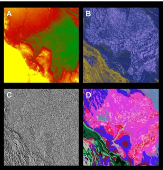
Figure 1. Fractional cover of photosynthetic vegetation (PV; green), non-photosynthetic vegetation (NPV; blue), and bare substrate (S; red) of our focal study region in Northern Peru.
The inset shows the location of the focal area within Peru. The region spans 16 million ha of ecological heterogeneity within the Maran˜on and Ucayali Watersheds. For carbon modeling purposes, airborne LiDAR data from CAO were divided using a checkerboard configuration, with 694,243 ha of calibration data (white) and 669,943 ha of validation data (black).
aboveground carbon density of all stems$10 cm in diameter (Mg C ha21
). This equation yields an R2of 0.84 and RMSE of 26 Mg C ha21
(see also [29]). The units of carbon estimated by this equation should be viewed for the purposes of this study as a consistent and reasonable output upon which to base the upscaling analyses for the region. Importantly, we emphasize that the present study is very unlikely to be influenced by the LiDAR calibration model used; Random Forest is a non-parametric algorithm, and any changes to the LiDAR-ACD calibration model would have a minimal impact on the magnitude of the ACD values and an even lower impact on the spread of those values.
Large-area data inputs
An overview of each large-scale input variables is provided in Table 1 and described in detail here; see also Figures 1, 2. Each data layer was prepared for Peru in its entirety, from which the focal area was subset.
First, we mosaicked ten 90-m resolution Shuttle Radar Topography Mission (SRTM) tiles [31] to produce a baseline elevation map of the focal area in Peru (Figure 2). The original data were resampled to 100-m resolution using pixel averaging, and from these data we produced topographic models of slope and aspect using a 363 sliding kernel (i.e., the slope or aspect of the
center pixel is calculated based on the elevations of all 9 pixels in the local environment of the center pixel).
Second, we processed 1071 Landsat 5 and Landsat 7 scenes (SLC off) taken in 2011 using Carnegie Landsat Analysis System lite (CLASlite). CLASlite automates radiometric correction and uses Monte Carlo Unmixing (MCU) to produce estimates of the percentage cover of soil, photosynthetic vegetation (PV), and non-photosynthetic vegetation (NPV) in every image pixel [32]. We used a pixel-selection algorithm (median Normalized Difference Vegetation Index, NDVI) to produce a ‘‘best-pixel’’ 2011 mosaic of 30 m-resolution MCU fractional cover. Due to persistent clouds in several regions, especially mid- and high-elevation forests, the resulting Landsat MCU mosaic lacked coverage for 2.4% of the
area. To plug these gaps, we mosaicked our Landsat fractional cover mosaic overtop of 500-m MCU output from MODIS. In this case, all MODIS fractional cover estimates were normalized with co-occurring Landsat pixels prior to mosaicking.
Finally, we incorporated a 134-class habitat map to represent geological and soil variation thought to regulate forest properties in Amazonian Peru and nearby regions [25,26,27,33]. The base input for this map was a national geological map for Peru to provide information on geologic and edaphic patterns in the study area [34]. Due to the importance of recent Quaternary fluvial features that were not included in the base map, we supplemented it with information from the NatureServe national vegetation map [35]. Lastly, we manually edited the geological map to account for recent findings on edaphic and floristic patterns in the region [25,33].
Upscaling methodology
We aligned all layers of the input data and resampled to 1-ha resolution using nearest neighbor resampling. We aligned corre-sponding 1.12-m resolution CAO LiDAR TCH data and determined average TCH in each 1-ha grid cell (follows [30]). From the large extent of the input data, we performed all upscaling on an area bounding the entire Maran˜on Watershed to avoid edge effects for our focal area of 16 million hectares.
Stratification. We stratified the input variables (Figures 1–2)
according to quantiles. Our goal was to produce as many unique (and useful) classes of habitat variation in order to map carbon variation among these classes [7]; however, an inordinately high number of breaks among the various input variables quickly results in too high a number of classes; ideally most classes will maintain a LiDAR sample of more than 100 ha or 1% [17,20], but in this case sampling was very dense (overall 8.5% of the focal area). We dispersed 20 bins non-randomly among our continuous input variables (i.e., STRM elevation, slope and aspect; CLASlite MCU soil, PV and NPV), based on the strength of those variables in influencing carbon stocks (Table 2). In previous studies, for
Table 1.Variables used to support three alternative upscaling methods for LiDAR-estimated tropical forest carbon stocks in a 16 million ha focal region in Northern Peru.
Upscaling method
Input Variable Explanation Stratification Random Forest
Random Forest with position
information
easting UTM X coordinate X
northing UTM Y coordinate X
diagx X coordinate after 45 degree clockwise image rotation X
diagy Y coordinate after 45 degree clockwise image rotation X
frac_soil Percent cover of soil as determined by Landsat image processing with CLASlite (%)
X
frac_pv Percent cover of photosynthetic vegetation as determined by Landsat image processing with CLASlite (%)
X X X
frac_npv Percent cover of non-photosynthetic vegeation as determined by Landsat image processing with CLASlite (%)
X X X
elevation SRTM elevation above sea level (m) X X X
slope SRTM slope (degrees) X X X
aspect SRTM aspect (degrees) X X X
geoeco Habitat class as determined by synthetic integration of national geological map, NatureServe and other sources
X X X
example, PV and elevation were found to be the primary controlling variables on carbon stock variation in Amazonian forests (follows [17]). We subsequently intersected all unique variable combinations with the 134-class habitat map. The
resulting classified map contained 8,035 classes. We intersected this class map with the CAO LiDAR data (for all of the Maran˜on region and surrounding environs, to avoid edge effects) to estimate median LiDAR-carbon content for each class; this median value was then mapped onto all pixels within that class using the class map.
Random Forest. We utilized the Random Forest algorithm
(as contained within the R package ‘‘randomForest’’ version 4.6– 7; R version 2.15.2 [36]) to produce a mapping prediction from the same input data layers as used in stratification. Although the Random Forest algorithm tested does include a built-in ‘‘out-of-bag’’ validation scheme, the effectiveness of this internal metric has not been tested with spatial data to our knowledge. Thus, to rigorously test Random Forest, we limited the model input data to a systematic subset based on a 50-km (on a side) grid cell (Figure 1). This limitation required the model to predict across large validation regions containing no input data. Combined, the focal region contained 36 calibration cells and 36 validation cells, providing a 50% leave out strategy—extremely conservative compared to most spatial modeling techniques (see, e.g., [37]).
We considered two separate ‘‘runs’’ of Random Forest, each using an identical set of 80,000 randomly selected input pixels among the calibration cells, which was at the limit of our computational resources. First, we produced a Random Forest model based on the large-scale input variables alone. Second, we produced a Random Forest model based on the input variables plus an additional four ‘‘position’’ parameters: x and y coordinates, combined with two diagonal coordinates (i.e., columns and rows for the image stack running from NW-to-SE and SW-to-NE, respectively). Position information can be critical in modeling underlying geographic trends within ecological data [38,39], and is now used in many examples of spatial modeling for purposes of predicting ecological trends [40–42]. We did not include such variables to imply any mechanistic control, but rather to serve the applied goal of accurately predicting carbon stock variation. We refer to this run of Random Forest throughout as that having ‘‘position information’’.
Model comparison and evaluation
We examined the resulting carbon maps side-by-side, first by considering differences among the maps. We then assessed performance by comparing the predicted ACD values within the 36 validation cells against LiDAR-observed ACD within those same cells. We used a distance transform of the extent of CAO calibration input data to determine whether the model perfor-mances were affected by increasing distance from CAO sample LiDAR data (Figure 3). The distance transform employed an approximate Euclidian distance algorithm which reproduces Euclidian distance effectively but is less computationally inten-sive—specifically ‘‘morph distance’’ in IDL (see also [43]).
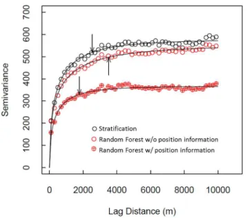
We also considered the spatial autocorrelation of each model’s residuals using two approaches. First, we created omnidirectional semivariograms (R package ‘‘geoR’’, version 1.7–3 [36]), which depict the correlation of observations according to increasing distance between those observations. Due to computational limitations, we created semivariograms using a random subset of 15,000 residuals (i.e., consistent spatially across all three upscaling approaches). Second, we applied Moran’s I, an index of spatial autocorrelation (R package ‘‘ape’’, version 3.0–8 [36]); Moran’s I ranges from21 to 1, where positive values indicate clumping and negative values indicate organized opposition (i.e., a chessboard pattern). Due to computational limitations, we assessed Moran’s I within a randomized subset of 5,000 observations (i.e., consistent spatially across upscaling approaches).
Table 2.Bin ranges for input variables used to produce a stratified map of the region over which carbon modeling was performed (see methods).
Soil PV NPV Elevation Slope Aspect
[0, 5) [0, 85) [0, 6) [0, 136) [0, 1.5) [0, Inf) [5, Inf) [85, 88) [6, 13) [136, 193) [1.5, Inf)
[88, 90) [13, Inf) [193, 443)
[90, 91) [443, Inf)
[91, 92) [92, 93) [93, 94) [94, Inf)
Twenty total bands were dispersed non-randomly according to the strength of each variable in predicting carbon stocks, which has been shown to be an effective stratification method in previous studies (e.g., [17]). Thereafter, the input variables were subset by quantiles to determine bin ranges for the bands. These class combinations were subsequently intersected with a 134-class habitat map as described in the methods, resulting in 8,035 unique classes within the focal area of the present study. A hard bracket indicates values ‘‘greater than or equal to’’, while a parenthesis indicates values that are ‘‘less than’’.
doi:10.1371/journal.pone.0085993.t002
Finally, we considered over-fitting by comparing the internal ‘‘out-of-bag’’ percent variation explained reported by the Random Forest algorithm to the percent variation explained in the 36 validation cells left out of the model input data.
Results
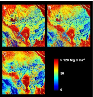
Stratification and Random Forest (both with and without position information) yielded predicted maps of ecosystem carbon stock that highlighted enormous variation across the 16 million-hectare focal area (Figure 4). The Pacaya-Samiria Swamp (center and east of the region) was generally modeled as containing low carbon stocks ranging from near 0 to,50 Mg C ha21, but also
showing considerable heterogeneity throughout the swampland. Upland terra firme forests were modeled consistently among the three approaches, including in the NE, SE, and NW corners of the focal area. However, several regions exhibited pronounced differences when using Random Forest with position information relative either to the other two approaches (Figure 5).
However, a clear benefit of using Random Forest with position information emerged during statistical comparison of the ap-proaches (Figure 6). As a baseline, stratification yielded a RMSE of 33.2 Mg C ha21
and adjusted r2 of 0.37 (predicted versus observed). A modest improvement was detected with Random Forest without position information (RMSE = 31.6 Mg C ha21, adjusted r2= 0.43), but the Random Forest model that included position information yielded a 20% improvement in RMSE (26.7 Mg C ha21
) and a 60% improvement in adjusted r2(0.59). The improvement when using Random Forest with position informa-tion appeared to be consistent at all distances from CAO LiDAR data (Figure 6).
We examined the net bias in each of the 36 validation cells separately by summing all residuals between predicted ACD and aircraft-observed ACD within each cell. In doing so, we found that Random Forest with position information out-performed both Stratification and Random Forest without position information in most cells (Figure 7). Notably, only one of 36 cells exhibited an
Figure 3. A distance transform map of the LiDAR-based carbon density calibration data used to evaluate the performance of the stratification and Random Forest models with increasing distance from aircraft observations. White areas indicate the greater distance from the calibration LiDAR flightlines in black. doi:10.1371/journal.pone.0085993.g003
Figure 4. Predicted carbon stocks using three different methodologies. (a) Stratification and mapping of median carbon stocks in each class, (b) Random Forest without the inclusion of position information, (c) Random Forest using additional model inputs for position.
doi:10.1371/journal.pone.0085993.g004
Figure 5. Three side-by-side carbon map comparisons. (a) Stratification minus Random Forest without position information, (b) Stratification minus Random Forest with position information, (c) Random Forest without position information minus Random Forest with position information. Areas consistently lower when position information is included (yellows in b and c) are largely low, inundated swamps and wetlands or mid-elevation pasturelands—all of which maintain high levels of photosynthetic vegetation cover (PV) but are comprised of lower carbon stocks in the airborne LiDAR data. Light blue areas (in b and c) are mostly low-elevation floodplain forests. See Discussion section regarding two annotated regions.
absolute net bias greater than 10 Mg C ha21
when using Random Forest with position information, and the overall distribution of bias among validation cells exhibited greater kurtosis (i.e., the distribution is more peaked around zero; Figure 7).
We found that the residuals of all three models were positively spatially autocorrelated; i.e., errors were spatially clustered (Figure 8). Moran’s I was highly significant in all cases (P%0.0001): Random Forest without position information
exhib-ited the highest Moran’s I (0.1466), followed by stratification (0.1155), and Random Forest with position information (0.1153). Finally, we detected over-fitting by Random Forest; both with and without position information, Random Forest’s internal ‘‘out-of-bag’’ percent variation explained was 29% greater than what the percentages determined using the 36 validation cells.
Discussion
Monitoring, reporting and verification is a critical part of any possible tropical forest carbon accounting system [11,44]. But
from individual landowners to entire nations, each jurisdictional entity must be able to determine not just how much carbon their land holds, but where that carbon is located. Ultimately, this means a spatially explicit, hectare-by-hectare capability is needed. We show here that Random Forest machine learning—if carefully implemented—can be a powerful spatial modeling tool to aid tropical forest carbon monitoring.
We evaluated two options for Random Forest, in the first case using a suite of input variables but lacking information on geographic position. This model performed similarly to the more traditional approach of stratification (sensu [7]), but it had some drawbacks that suggest high risk: model fit to validation data was somewhat better than stratification (i.e., modest decrease in RMSE and increase in adjusted r2), but a downside was increased spatial autocorrelation among the model residuals, as measured by a 27% increase in Moran’s I when using Random Forest.
However, the second option, which included the same suite of input variables as well as four position parameters, produced much more accurate results with validation data compared to the
Figure 6. Performance of three modeling techniques as assessed in 36 validation cells.Left panels highlight model performance against LiDAR-observed aboveground carbon density from CAO aircraft data (Mg C ha21), while right panels highlight the model performance by increasing
distance from CAO aircraft data. The color-scale reflects the two-dimensional density of observations, adjusted to one dimension using a square root transformation.
stratification approach, and without increasing spatial autocorre-lation in the residuals. Side-by-side comparison of the carbon maps resulting from the three techniques provides some insight into the improvement in model predictions when pixel position is included (Figure 5). Within the Pacaya-Samiria swampland in the focal area, for example, a band of floodplain forests several kilometers wide follows the Ucayali River (annotation 1 in Figure 5); these forests have high carbon stocks in LiDAR data, but occupy a very low-lying area relative to the rest of the focal area, and they appear to have common elevation, slope, and greenness to lower-carbon swamps and marshes elsewhere in the swampland. Similarly, context-dependent patterns appear to influence carbon stocks in the southwest portion of the focal area (annotation 2 in Figure 5). Here, high elevation forested valleys have relatively high predicted carbon stocks in all three models,
but nearby east-facing mountain slopes maintain high greenness yet exhibit lower carbon stocks in LiDAR data; these areas have much lower predicted carbon stocks when position information is included in the Random Forest model. Ecologically, the results suggest that relative rather than absolute elevation may be more predictive of localized variation in carbon stocks in many instances throughout the region.
Our results suggest that the inclusion of position information is helpful—and potentially critical—to advancing Random Forest as an upscaling and modeling approach for tropical forest carbon mapping. With position information as model input variables, we suggest that Random Forest is better able to account for the context in carbon stock patterns—i.e., spatial autocorrelation of observed carbon stocks in LiDAR data—increasing its predictive accuracy in unseen data. To our knowledge, although Random
Figure 7. Spatial performance of each modeling approach within 36 validation regions.The net bias for the model was determined against the aircraft-based observed validation data (i.e., 1-ha CAO aircraft samples shown in black in figure 1). The color-scale is defined within the histograms, and is constant in all panels.
Forest has been used in several ecological and spatial studies to date, position information has yet to be included in any predictive model of carbon or other ecological parameter [4,16,22,23]. Our results suggest that future efforts should make better use of position information in order to improve predictive power and possibly better account for spatial autocorrelation. In principle, including position information in the stratification approach might lead to a similar improvement in performance. However, unlike Random Forest, the stratification approach lacks an algorithm to decon-struct which position information that is relevant to ACD patterns and which is not. Given that 8,035 classes were created from the intersection of the limited variable set considered in this case, the rapidly increasing number of classes may quickly make the exercise intractable.
Does Random Forest over fit to spatial data? Our results suggest that it does. Random Forest leaves out portions of the input data (called ‘‘out-of-bag’’) to evaluate its prediction and this approach is theoretically less prone to over fitting to training data compared to other machine learning algorithms [22]. But, in implementing both instances of Random Forest here, the ‘‘out-of-bag’’ predictive power generated by the model was 29% higher than what we
determined for validation areas never included at any stage. Ultimately, while over-fitting is not desirable, Random Forest with position information still produced the best results in unobserved areas as assessed by validation data (Figure 7). This suggests that care must be taken when using Random Forest with spatial data and that the internal ‘‘out-of-bag’’ feature appears not to be robust to spatial data.
Our mapping predictions exhibited spatial autocorrelation of errors, as has been the case with most other regional-, jurisdictional- and national-scale carbon mapping efforts. While including position information as input variables in Random Forest did reduce spatial autocorrelation, it did not eliminate it (i.e., Moran’s I declined from 0.1466 to 0.1153, which was a difference outside the standard deviation of each Moran’s I estimate). With position information, Random Forest exhibited no statistical difference in spatial autocorrelation from the stratifica-tion approach (at a Moran’s I of 0.1155), yet produced a major improvement in model performance in terms of RMSE and r2in validation data. Although the spatial autocorrelation of errors is undesirable, Random Forest with position information provided an improvement over stratification, and maintained the same spatial autocorrelation as with stratification.
Machine-learning algorithms have the potential to substantially improve spatial modeling of carbon stocks in tropical forests and possibly other ecosystems. Although some drawbacks remain unresolved—namely over-fitting and spatial autocorrelation of model errors—Random Forest may provide a viable pathway to improve large-area modeling of carbon stocks over existing methods such as stratification. This is particularly true in large-scale, high-resolution modeling exercises that are currently intractable when using parametric statistical approaches such as simultaneous autoregressive modeling due to computational limitations (e.g., SAR [37,45]). We emphasize that our modeling outcomes greatly benefited from an unprecedentedly high density of airborne LiDAR data over a large geographic region, and this suggests that high data density may be critical moving forward. Further, testing Random Forest against other modeling approach-es beyond stratification (e.g., k-nearapproach-est neighbor, maximum entropy) is also critical to determine its ultimate utility in carbon mapping.
Acknowledgments
The manuscript was greatly improved by comments from two anonymous reviewers, as well as insight from M. Colgan and F. Collman.
Author Contributions
Conceived and designed the experiments: JM GPA DEK. Performed the experiments: JM GPA DEK. Analyzed the data: JM GPA DEK TK REM CA MH KDC. Wrote the paper: JM GPA.
References
1. Fanelli G, Gall J, Van Gool L (2011) Real time head pose estimation with random regression forests. In Computer Vision and Pattern Recognition (CVPR), 2011 IEEE Conference. pp. 617–624.
2. Triebel R, Grimmett H, Paul R, Posner I (2013) Introspective Active Learning for Scalable Semantic Mapping. Workshop on Active Learning in Robotics: Exploration, Curiosity and Interaction. Robotics Science and Systems. 3. Breiman L (2001) Random forests. Machine Learning 45: 5–32.
4. Baccini A, Goetz SJ, Walker WS, Laporte NT, Sun M, et al. (2012) Estimated carbon dioxide emissions from tropical deforestation improved by carbon-density maps. Nature Climate Change 2: 182–185.
5. Evans JS, Murphy MA, Holden ZA, Cushman SA (2011) Modeling species distribution and change using random forest. In: Drew CA, Wiersma YF, Huettmann F, editors. Predictive species and habitat modeling in landscape ecology: concepts and applications. New York City, NY, , USA: Springer Science+Business Media. pp. 139–159.
6. Breiman L (2001) Statistical modeling: The two cultures (with comments and a rejoinder by the author). Statistical Science 16: 199–231.
7. Asner GP (2009) Tropical forest carbon assessment: integrating satellite and airborne mapping approaches. Environmental Research Letters 4: 034009. 8. Colgan MS, Asner GP, Swemmer T (2013) Harvesting tree biomass at the
stand-level to assess the accuracy of field and airborne biomass estimation in savannas. Ecological Applications: 23:1170–1184.
9. Martin AR, Thomas SC (2011) A reassessment of carbon content in tropical trees. PLoS One 6: e23533.
10. Chave J, Andalo C, Brown S, Cairns MA, Chambers JQ, et al. (2005) Tree allometry and improved estimation of carbon stocks and balance in tropical forests. Oecologia 145: 87–99.
11. Angelsen A (2008) Moving Ahead with REDD: issues, options and implications. Bogor, Indonesia: Center for International Forestry Research (CIFOR). 156p.
Figure 8. Variograms of residuals from three model predictions of carbon stock in the focal area: Stratification (black circles), Random Forest without position information (red open circles), and Random Forest with position information (red circles with target). Fitted curves are weibull functions, and the arrows indicate a y-axis value of 90% of the fitted asymptote (i.e., the ‘‘a’’ parameter in the weibull function).
12. Drake JB, Knox RG, Dubayah RO, Clark DB, Condit R, et al. (2003) Above-ground biomass estimation in closed canopy neotropical forests using lidar remote sensing: Factors affecting the generality of relationships. Global Ecology and Biogeography 12: 147–159.
13. Ene LT, Naesset E, Gobakken T, Gregoire TG, Stahl G, et al. (2012) Assessing the accuracy of regional LiDAR-based biomass estimation using a simulation approach. Remote Sensing of Environment 123: 579–592.
14. Asner GP, Powell GVN, Mascaro J, Knapp DE, Clark JK, et al. (2010) High-resolution forest carbon stocks and emissions in the Amazon. Proceedings of the National Academy of Sciences 107: 16738–16742.
15. Saatchi SS, Harris NL, Brown S, Lefsky M, Mitchard ETA, et al. (2011) Benchmark map of forest carbon stocks in tropical regions across three continents. Proceedings of the National Academy of Sciences of the United States of America 108: 9899–9904.
16. Hudak AT, Strand EK, Vierling LA, Byrne JC, Eitel JUH, et al. (2012) Quantifying aboveground forest carbon pools and fluxes from repeat LiDAR surveys. Remote Sensing of Environment 123: 25–40.
17. Asner GP, Clark JK, Mascaro J, Galindo Garcı´a GA, Chadwick KD, et al. (2012) High-resolution mapping of forest carbon stocks in the Colombian Amazon. Biogeosciences 9: 2683–2696.
18. Asner GP, Hughes RF, Mascaro J, Uowolo A, Knapp DE, et al. (2011) High-resolution carbon mapping on the million-hectare Island of Hawai’i. Frontiers in Ecology and the Environment 9: 434–439.
19. Mascaro J, Asner GP, Muller-Landau HC, Van Breugel M, Hall J, et al. (2011) Controls over aboveground forest carbon density on Barro Colorado Island, Panama. Biogeosciences 8: 1615–1629.
20. Asner GP, Clark JK, Mascaro J, Vaudry R, Chadwick KD, et al. (2012) Human and environmental controls over aboveground carbon storage in Madagascar. Carbon balance and management 7: doi:10.1186/1750-0680-1187-1182. 21. Asner GP, Mascaro J, Anderson C, Knapp DE, Martin RE, Kennedy-Bowdoin
T, et al. (2013) High-fidelity national carbon mapping for resource management and REDD+. Carbon balance and management 8: 1–14.
22. Cutler DR, Edwards TC, Jr., Beard KH, Cutler A, Hess KT (2007) Random forests for classification in ecology. Ecology 88: 2783–2792.
23. Rodriguez-Galiano VF, Abarca-Hernandez F, Ghimire B, Chica-Olmo M, Atkinson PM, et al. (2011) Incorporating Spatial Variability Measures in Land-cover Classification using Random Forest. In: Stein A, Pebesma E, Heuvelink G, editors. 1st
Conference on Spatial Statistics 2011 - Mapping Global Change. pp. 44–49.
24. ter Steege H, Pitman NCA, Phillips OL, Chave J, Sabatier D, et al. (2006) Continental-scale patterns of canopy tree composition and function across Amazonia. Nature 443: 444–447.
25. Tuomisto H, Ruokolainen K, Yli-Halla M (2003) Dispersal, environmental, and floristic variation of western Amazon forests. Science 299: 241–244. 26. Tuomisto H, Ruokolainen K, Kalliola R, Linna A, Danjoy W, et al. (1995)
Dissecting Amazonian biodiversity. Science 269: 63–66.
27. Higgins MA, Ruokolainen K, Tuomisto H, Llerena N, Cardenas G, et al. (2011) Geological control of floristic composition in Amazonian forests. Journal of Biogeography 38: 2136–2149.
28. Asner GP, Knapp DE, Boardman J, Green RO, Kennedy-Bowdoin T, et al. (2012) Carnegie Airborne Observatory-2: Increasing science data dimensionality via high-fidelity multi-sensor fusion. Remote Sensing of Environment 124: 454– 465.
29. Asner GP, Mascaro J, Muller-Landau HC, Vieilledent G, Vaudry R, et al. (2012) A universal airborne LiDAR approach for tropical forest carbon mapping. Oecologia 168: 1147–1160.
30. Asner GP, Mascaro J (2013) Mapping tropical forest carbon: Calibrating plot estimates to a simple LiDAR metric. Remote Sensing of Environment 140:614– 624.
31. Jarvis A, Reuter HI, Nelson A, Guevara E (2008) Hole-filled seamless SRTM data V4. International Centre for Tropical Agriculture (CIAT). http://srtm.csi. cgiar.org.
32. Asner GP, Knapp DE, Balaji A, Paez-Acosta G (2009) Automated mapping of tropical deforestation and forest degradation: CLASlite. Journal of Applied Remote Sensing 3: 033543.
33. Higgins MA, Asner GP, Perez E, Elespuru N, Tuomisto H, et al. (2012) Use of Landsat and SRTM data to detect broad-scale biodiversity patterns in Northwestern Amazonia. Remote Sensing 4: 2401–2418.
34. INGEMMET (2000) Geolo´gico del Peru´. Lima, Peru: Instituto Geologico Minero Y Metalurgico.
35. Josse C, Navarro G, Encarnacio´n F, Tovar A, Comer P, et al. (2007) Ecological Systems of the Amazon Basin of Peru and Bolivia. Arlington, Virginia, USA: NatureServe.
36. R Core Team (2013). R: A language and environment for statistical computing. Vienna, Austria: R Foundation for Statistical Computing.
37. Dahlin KM, Asner GP, Field CB (2012) Environmental filtering and land-use history drive patterns in biomass accumulation in a mediterranean-type landscape. Ecological Applications 22: 104–118.
38. Miller J, Franklin J, Aspinall R (2007) Incorporating spatial dependence in predictive vegetation models. Ecological Modelling 202: 225–242.
39. Legendre P, Legendre L (1998) Numerical Ecology: second english edition. Developments in Environmental Modelling: 20.
40. Dahlin KM, Asner GP, Field CB (2012) Environmental filtering and land-use history drive patterns in biomass accumulation in a mediterranean-type landscape. Ecological Applications 22: 104–118.
41. Dahlin KM, Asner GP, Field CB (2013) Environmental and community controls on plant canopy chemistry in a Mediterranean-type ecosystem. Proceedings of the National Academy of Sciences 110: 6895–6900.
42. Hudak AT, Crookston NL, Evans JS, Hall DE, Falkowski MJ (2008) Nearest neighbor imputation of species-level, plot-scale forest structure attributes from LiDAR data. Remote Sensing of Environment 112: 2232–2245.
43. Fabbri R, Costa LDF, Torelli JC, Bruno OM (2008) 2D Euclidian distance transform algorithms: a comparative survey. ACM Computing Surveys 40: 1– 44.
44. Herold M, Skutsch M (2011) Monitoring, reporting and verification for national REDD+ programmes: two proposals. Environmental Research Letters 6: 014002.