Abstract—Product innovations, accelerated product life cycles, globalization, and increased customer requirements are challenges of the automotive industry today. Original equipment manufacturers face these challenges in offering multiple models, derivates, and options that affect the efficiency of processes and resources in logistics systems. To provide transparency over product variety-induced complexity, individual product variants, product variety and their impacts on logistics costs and performance need to be linked. Against this background, the authors develop an evaluation method to quantify these impacts focusing on the automotive logistics.
This research provides a structured framework to account for impacts caused by product variety in order to support product variety decisions at an early stage in the product design phase. The method identifies relevant influences for measuring variant-driven complexity in logistics and highlights reciprocal effects among product variety, logistics costs and logistics performance. By integrating different logistics resources as well as dynamic factors, the research provides a unique evaluation approach in automotive logistics. Furthermore, the authors provide a case study proving the practicability.
Index Terms—Automotive Logistics, Complexity, Product Variety, Activity-based Costing
I. INTRODUCTION
Globalization and market saturation leading to an increased competition, product innovations, and accelerated product life cycles are challenges of the automotive industry at the beginning of this century [1]. Furthermore, increased customer demands that require individuality in terms of options and configurations of automobiles at decreased
Manuscript received December 8, 2010; revised January 14, 2011. The Authors gratefully acknowledge the research CAPES / DFG (BRAGECRIM project IDELN / HeliOPP) for their support.
A. Lechner is a researcher with the Fraunhofer Institute for Material Flow and Logistics, Joseph-von-Fraunhofer-Str. 2-4, 44227 Dortmund, Germany (phone: +49(0)231-9743283; fax: +49(0)231-974377283; e-mail: annika.lechner@ iml.fraunhofer.de).
K. Klingebiel is the head of the Research Center for Logistics Assistance Systems at the Chair of Factory Organization, Technical University of Dortmund, Leonard-Euler-Str. 5, 44227 Dortmund, Germany (e-mail: [email protected]).
A. Wagenitz is the head of the department Supply Chain Engineering at the Fraunhofer Institute for Material Flow and Logistics, Joseph-von-Fraunhofer-Str. 2-4, 44227 Dortmund, Germany (e-mail: [email protected]).
customer reservation prices and variable customer demands characterize the automotive environment [2]. As a reaction, original equipment manufacturers (OEM) have and will considerably enlarge their model and option range [3]. This rise in number of product variants leads to an increased product variety that affects processes and resources in logistics systems [4]. The problems in logistics systems are lacking transparency regarding these impacts on costs and performance due to the interaction between logistics system elements and product variety, e.g. concerning capacities [5].
To evaluate logistics strategies at an early stage in the product design phase, e.g. the determination of an optimal order penetration point, knowledge over product variety’s impacts is a requisite. In order to provide transparency over product variety’s impacts, relevant influencing factors have to be identified and quantified in terms of costs and performance. Variant costs, often referred to as complexity costs, are generally regarded as overhead costs and are consequently accepted as fix costs. These fix costs account for the majority of supply chain costs [6]. In practice, volume effects of variants are overestimated, whereas their impacts on costs remain underestimated [7]. As a result, costs that are assigned to variants are too low [8]. Therefore, variant costs are often considered as hidden costs of doing business [9]. Hence, this research aims at developing an evaluation method, underlying the idea of Time-driven Activity-based Costing and a zero-base approach, which allocates overhead costs to the level of product variety according to the actual input involved.
The analysis presented in this research paper is the first of two modules towards the development of a model-based evaluation approach of variant-driven complexity in the automotive industry by capturing relevant product variety-driven costs and performance impacts. The proposed method builds the basis for an efficient evaluation of strategic decisions even at an early stage in the product design phase in terms of product variety.
This research paper is divided into five main chapters including this introduction. A literature review with related work is given in Chapter 2, whereas Chapter 3 comprises the development of the Variety-driven Activity-based Costing (VD-ABC). Chapter 4 presents a case study to evaluate the proposed method at a German OEM. The authors conclude in Chapter 5 with a final discussion and a summary of findings.
Evaluation of Product Variant-driven
Complexity Costs and Performance Impacts in
the Automotive Logistics with Variety-driven
Activity-based Costing
II. RELATED WORK
Publications in engineering, science, economics, business management as well as social sciences, use numerous definitions of the term complexity. A comprehensive overview over theories and interpretations of complexity is given by Meyer, Kirchhoff, and Specht, whereas Wu, Fredendall, and Frizelle give an overview over production engineering complexity theories [10]-[14]. In systems theory complexity is defined as a system characteristic described by the number of elements, their relations, and the transformation of elements and relations over time [10]. Static or structural complexity arises from the system structure, whereas the dynamic or operative complexity addresses the system behavior over time [7].In the context of automotive logistics, product variety is the known phenomenon of complexity [11]. Product variety not only affects logistics costs and performance, but also the design of logistics systems. A logistics system is any configuration of at least two logistics elements (e.g. parts) to plan, control, and monitor. Its structure comprises knots (e.g. production sites) and connections between the knots (e.g. transport routes) and serves the accomplishment of logistics processes [15].
Within the scope of this research, product variety-driven complexity in logistics systems is defined combining multiple system theoretic definitions as a system characteristic described by the number and variety of product variants, their relations among each other, and the transformation of elements and relations over time, which influences logistics costs and performance.
A. Methods to Evaluate Complexity
To evaluate impacts of an increasing product variety in logistics, evaluation approaches that address logistics costs and performance are examined at this point. The cost evaluation of variants and variety-induced complexity found much interest in research, whereas the performance evaluation has not been considered in logistics. Approaches to calculate variant costs vary in terms of the level of detail, the field of application, and the corresponding approach. The oldest approach to calculate variant costs is the overhead calculation by Pfeiffer, which allows a cost allocation to variant-rich products through an adjusted overhead allocation [16]. The overhead calculation addresses the problem that variant costs are mainly found in overhead costs. However, Pfeiffer only allocates product costs based on volumes. As a result, costs for variants with low volumes are underestimated.
Consequently, the Activity-based Costing (ABC) has been developed aiming a cost allocation to objects fair according to the input involved [17]. Evaluation approaches to calculate variant costs are often based upon ABC. The cost-benefit evaluation of variety of Heina and Puhl comprises a variant calculation method based on a classic ABC [18], [19]. Their calculation distinguishes between standard and variant attributes of objects. Variant costs are calculated with average rates subject to the volume instead of variant-specific cost rates. However, process times in variant-rich automotive logistics systems differ significantly
subject to product variety. The resource-oriented ABC (RPK) avoids this simplification in allowing detailed cost drivers for sub-processes. Schuh developed a model, which quantifies the variant-specific consumption of resources with cost and usage functions [7]. However, this implies a comprehensive data collection and a high update effort.
To avoid a comprehensive data collection, Kaplan and Anderson developed the Time-driven ABC (TD-ABC) [20]. TD-ABC uses time functions, which potentially allow the allocation of different consumption rates to different product variants. TD-ABC determines resource demands and hence costs based on time functions. Everaert et al.
applied this method to calculate logistics costs at a wholesaler [21]. Within the scope of the research project BAU-MO, a TD-ABC model was developed to evaluate variants in the construction machinery industry [22], [23]. The model is based upon cost drivers. However, proposed time functions are subject to individual variants and neglect the overall level of variety.
Besides these process-oriented approaches to evaluate variant costs, there are further static evaluation approaches. Schaffer developed a complexity cost model to capture the complexity costs structure in the automotive production [24]. He identified complexity cost types and calculates cost rates for different cost drivers on an automobile level. Cost rates are developed using cost structures. Further, Wulfsberg and Schneider present a variant cost tool on the basis of the Fuzzy Set Theory with a fuzzy quantification of variant costs [25]. Rosenberg developed an approach to determine the cost effectiveness of complexity-changing activities from a financial point of view, where costs are calculated as reduced or additional costs [26]. Bohne developed a theoretical complexity cost analysis with a zero-base analysis [27]. On the basis of variant-free activities, resource demands of each cost center in research and development, sales, marketing, and production are analytically redesigned. Further, Lackes developed a production attribute-oriented variant standard costing on the basis of a flexible cost accounting [28].
B. Discussion and Research Question
Existing evaluation approaches that consider product variety in their costing determine variant-induced percentages on the basis of estimates or fixed ratios. However, this allocation is not fair according to the actual input involved. For instance, Schaffer estimates the complexity-induced ratio with a complexity factor; the BAU-MO approach distinguishes processes according to their level of interference with variety in strong, medium or low. Often, these estimates are based on interviews.
intensive planning, control and coordination processes in the automotive industry are not considered. This focal point on partial costs leads to escalated capacity adaptations through an unknown incremental increase of capacity demands, which only become apparent after it is too late.
Summarizing, existing evaluation methods either show no connection between variety-induced logistics costs and their impacts on the logistics performance, are based on estimates or cannot be adjusted to the application area. Against this background, these deficits lead to the following research question: What is the design of an evaluation approach to assess product variety-driven complexity in order to quantify the impacts of product variety on logistics costs and logistics performance without relying on estimates?
Hence, this research aims at developing an evaluation approach, which allocates costs, in particular overhead costs, to the level of product variety according to the actual input involved. The challenge is the development of a method that is not based on estimates. The author’s idea is the relative indication of complexity to a hypothetic zero-variant-scenario on the basis of Bohne’s zero-base analysis and Kaplan and Anderson’s TD-ABC. The combination of the two methods offers the potential to connect variety resource demands in automotive logistics, costs, and performance impacts without being based upon estimates. Consequently, these methods have to be specified according to context-specific requirements.
III. VARIETY-DRIVEN ACTIVITY-BASED COSTING
In terms of product variety and complexity, the automotive industry takes up a leading role. On the one hand, automobiles are complex products with complex product structures [29]. The total number of product variations in automobiles even exceeds the number of 1020 for several models of the German automotive premium segment, e.g. BMW, Audi, and Mercedes models [30]. On the other hand, automotive logistics systems are complex systems due to their high number of system elements, relations, and transformations over time [7]. Typical elements are products (e.g. parts, modules) or resources (personnel, space, means of transportation, etc.).
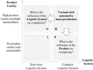
Dependent on product variety and the logistics systems, the authors distinguish between four product-system types, which are displayed in Fig. 1. The matrix differentiates between the level of product variety, i.e. automobile variety and the level of complexity of the logistics system. Existing automotive logistics systems within a variant-rich mass production are classified as complex systems with complex products (iii).
Given this background, the authors ask the following questions: What is the influence of the product and what is the influence of the logistics system on complexity? As product variety is considered as the core source of complexity, the focus of this research paper is to capture the influence of the product. The authors limit their research to the first question in developing a calculation method based on product variety changes.
iv
ii iii
i
Product Variety
High product variety (multiple
automobiles)
No product variety (one automobile)
Zero-base Logistics System
Complex Logistics System
Logistics System Variant-rich
automotive mass production
What is the influence of the
Producton complexity? What is the
influence of the
Logistic System
on complexity?
Fig. 1. Classification of Products and Logistics Systems
Consequently, the logistics system remains unchanged in this analysis, whereas different levels of product variety, ranging from zero variants to multiple variants, are analyzed. With a zero-variety approach, base and variant parts of an automobile are identified. This influence of the product and product variety respectively is determined by comparing costs of a logistics system producing variant automobiles to costs of the same logistics system producing just one base automobile as end product. In the context of time, the proposed evaluation represents a short-term evaluation as logistics structures cannot be changed quickly [31].
A. From TD-ABC to VD-ABC
To capture the demand according to variants, the authors propose an enhanced costing method, which is based upon the idea of TD-ABC [20]. To account for characteristics in automotive logistics systems, in particular product variety, the concept of ABC has been adjusted. In applying TD-ABC, two parameters have to be determined:
- Capacity cost rate as the ratio of costs of capacity supplied and the practical capacity of resources supplied
- Capacity demand rates
For logistics processes, the practical capacity is expressed as the amount of time that employees can work, without overtime. By dividing total costs by the practical capacity, costs per unit of time are calculated. These are assigned to orders by multiplying the costs per unit of time with the time needed to perform the process. These resource or capacity demands respectively are calculated using process time equations (1). The authors define the standard process time t0, the process time of incremental activity i as ti, and the number of incremental activities xi. The variable yi is a binary variable which equals 1 if an incremental activity is necessary and zero otherwise.
v v
vx y
t y x t y x t t
times process individual
of sum time process
2 2 2 1 1 1 0
(1)
intensive data collection and allocation to cost drivers as is the case in other process-oriented evaluation methods.
TD-ABC has not been developed to calculate variety-driven logistics complexity costs in particular. This transformation is achieved within the scope of this research. Through the differentiation of automobile parts into base and variant parts, a reference scenario with zero variants is created, which allows the comparison to existing scenarios with variety.
Resources of a logistics system include floor space, personnel, inventory, equipment, auxiliary equipment, and organisational equipment [32]. These logistics resources are occupied and consumed during the transformation of logistics objects - product variants - in processes. To calculate costs which occur through the consumption of logistics resources, the authors introduce the concept of Variety-driven Activity-based Costing (ABC). VD-ABC uses the capacity cost rate to drive overhead costs to variants by determining the demand for logistics resource capacity subject to product variety. With process equations based on the concept of TD-ABC, the resource consumption of personnel and equipment is captured as these resource costs are directly dependent on the consumed time. However, as TD-ABC only comprises capacities in terms of units of time, it is impossible to capture demands of the logistics resources inventory and floor space with process equations. Yet, this is evident to account for all relevant costs of a logistics system according to [32]. Consequently, the authors expand the concept of TD-ABC to capture capacities in parts and square meter, which cannot be measured in units of time. Against this background, the authors developed the following three capacity equations, which build the heart of VD-ABC:
- Process time equations are modeled for each process assigning each sub-process an individual time depending on product variety. Process equations account for demands of the logistics resources personnel and equipment as their consumption is dependent on time. From an intensity point of view, process times become adjusted to the degree of the handled product’s complexity, i.e. product variety. - Inventory equations are modeled assigning individual
inventory levels to variants depending on the inventory strategy and product variety.
- Floor space equations are modeled for each process, assigning each variant’s sub-process individual space demands subject to product variety.
The capacity equations comprise the base capacity consumption and terms of additive incremental capacity consumption. Whereas the base capacity is needed in a zero-variant-scenario, incremental capacities are required in a variety-scenario. Consequently, the capacity equations of VD-ABC capture resource demands for different levels of product variety bottom-up. Capacity equations are not interdependent and interact with each other.
Variant-driven complexity costs are obtained using the capacity equations. The difference between a scenario having v variants and a zero-variant-scenario is considered as variant-driven complexity and therefore quantified in terms of complexity costs for each variant and resource.
Summing up the complexity costs over all logistics resources, the overall complexity costs in a variety-scenario are quantified.
B. Variety Process Equation
The adaptation of TD-ABC to account for product variety is addressed in the following. Processes and products correlate in three ways: process content, process type and number of processes. Additional costs due to variants occur for processes, which are only necessary in variant-rich logistics systems (e.g. a sequencing process) as well as for processes, which become more laborious and thus increase the throughput time and resource demands. Due to the scalability of the proposed process functions, processes on different levels, i.e. sub-processes and main processes are determined. Variant-induced resource demands of personnel and all types of equipment for one variant are determined using process time equations (2).
v vy t y t y t t
TP 0 1 1 2 2 (2)
This principle allows the allocation of individual demands to variants. The authors define time t for process P for one variant v as TP in units of time (TU), the total number of variants and product variety respectively as V with the range of variant v = 1,…,V. The variable yv is a binary variable which equals 1 if the sub-process is necessary for variant v and zero otherwise. In the context of logistics material flow systems of the automotive mass production, differences in process times between individual variants are not significant as shown in Fig. 2.
0 2 4 6 8 10
ba se pa rt va ria nt 1 va riant 2 va ria nt 3
P
ro
ces
s T
im
e
(T
U
)
Va ria nt Fig. 2. Process Times dependent on the Variant
This is explained by the similarity of product variants in terms of logistics handling. Hence, resource costs for individual product variants do not vary. This variant behavior differs from other industry’s variant processes, e.g. the construction industry, where process times vary with each variant as variants and products respectively are all individual.
0 2 4 6 8 10 12 14 16
base parts: 0 variants 1 additional variant 2 additional variants 3 additional variants P ro c e ss T im e ( T U )
Va ria nt Scena rio
additional capacity demand (AC)
base capacity demand
AC1= + 2 TU
AC2= + 4 TU
AC3= + 6 TU
Fig. 3. Process Times subject to Product Variety
The corresponding process equations subject to the number of variants and thus product variety are shown in (3). For variety process equations the authors define the time for process P in a logistics system with v variants TPv , the process time referring to a specific variant as tv, the additional capacity demand time for v variants ACv, and the number of parts per variant v per unit of time at V as V
v x . v to due increase time AC x x t x t TP x x x t x t x t x t TP x t TP v V v v V V v V
( ) ) ( 0 0 1 1 1 0 0 0 0 0 1 1 1 1 1 0 0 0 1 1 1 1 0 0 1 0 0 0 0 (3)
At this point, step-fix costs which occur due to variety increases are of interest. Step-fix costs arise based on process type changes as well as based on an intensification of the process work content. They occur if capacities are limited and insufficient due to unsteady capacity increases. An increased time demand requires additional personnel and equipment capacities. These capacity adaptations are not steadily increasing with the demand, but rather occur in discrete steps.
Capacity cost rates of all logistics resources are calculated by dividing the total resource costs by the practical capacity supplied. The difference between a scenario having v variants and a zero-variant-scenario with v = 0 constitutes the variant-driven complexity costs. The authors further define complexity costs CC for all logistics resources R, the total costs of resource R as CR, the practical capacity of R as cR, and the capacity cost rate of R as CRR. Then, variety-driven complexity costs for personnel CCP and equipment CCE are calculated as follows:
R R R v R v R R v c C CR AC CC with CC
CC
/ (4)Moreover, impacts on the throughput time as the essential component of the logistics performance are depicted with the proposed process equations. As long and variable throughput times counteract a high delivery service, the method even allows qualitative conclusions to the delivery service [33].
C. Variety Inventory and Floor Space Equations
At the OEM, inventory is distinguished in stock of inventory and work-in-progress (WIP). WIP can be calculated according to process equations. However, this is impossible for stocks. With an increase of product variety, higher inventories of stocks at several stages along the supply chain are needed [34]. This leads to increased stock keeping costs, as stock-outs for each individual variant have to be prevented. In reverse, the consolidation of individual stocks leads to a lower overall stock. This concept is known as variability pooling [35]. The same concept can be applied to the reduction and increase of product variety. To capture this effect on the logistics resource inventory, relevant influencing factors on inventory are identified being the number of variants and demand variations [36].
Inventory equations are modeled to indicate the inventory development as a function of product variety. According to process equations, inventory equations consist of the base inventory and additive incremental inventories. For this purpose the authors use the safety stock concept of the Newsvendor Model, which calculates inventories according to demand variations, the number of variants and the service level [37], [35]. Given a scenario with zero variants, no safety stocks have to be hold due to demand variability because a constant number of parts is required per unit of time. For example, all automobiles need one windshield. Given that windshields are compulsory variants, the demand of this particular windshield is constant as the windshield is assembled for all cars. Consequently, the required inventory comes to the average demand. However, in a scenario with several windshield variants, a higher safety-stock is needed for each variant to prevent stock-outs as demands are variable. It can be stated that the more variants, the lower the average demands and the higher demand volatility. To calculate demands, it is appropriate to assume normally distributed demand variations [38].
The proposed variety inventory equations are given in (5) capturing the inventory of stock and inventory costs (6). The authors define the inventory in a V-variant-scenario as Iv, the mean demand of variant v in a scenario of V variants per unit of time and the corresponding demand standard variation V
v
and V
v
respectively. The parameter z is chosen from statistic tables to make sure the probability of this variants stock out is above a certain service level.
v to due inventory additional AI z I z z I z I v V v V v V
10 0 1 1 1 0 0 0 1 1 1 0 1 1 1 0 1 0 0 0 0 0 0 0 ) ( ) (
(5)
With increased inventories, additional capital is tied up at the OEM as innovative payment concepts are just about to develop (Pay-on-Production, Supplier-Managed-Inventory, etc.) [39]. Inventory stock costs CIv are dependent on the interest rate r and on the variant’s purchased prices V
v
e ,
supplier faces additional costs due to decreased lot sizes and costly variants. Therefore, variety-induced inventory complexity costs CCIV for v variants are calculated as opportunity costs due to an additional capital lockup. CCI1 for example represents the incremental cost increase due to one variant as shown in (6).
1 1 1 1 0 1 0 1 1 1 1 1 1 1 0 0 0 1 0 0 0 0 0 )] ( ) ( [ CCI z e z e r r e CI r e CI (6)
As inventories largely determine the required floor space, variety floor space equations are developed in the same way. According to the quantification of complexity costs for process equations, floor space complexity costs are determined.
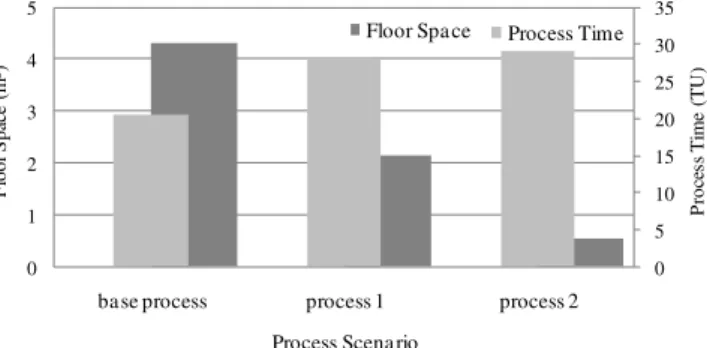
Variety process, inventory and floor space equations need not to be examined independently, but have to be captured simultaneously to account for the overall complexity (see Fig. 4). With this, the consequences of product differentiation and reduction of lot sizes along the supply chain are captured in comparing a zero-variant-scenario with a variety scenario with respect to floor space and process time. 0 5 10 15 20 25 30 35 0 1 2 3 4 5
base process process 1 process 2
P ro ces s T ime ( T U ) Fl o o r Sp ac e (m ²)
Process Scena rio
Floor Spa ceFloor Spa ce Process Time
Fig. 4. Interaction of Capacity Equations using the example of Variety Process Equations and Floor Space Equations subject to processes
IV. PRACTICAL EVALUATION OF THE METHOD
In this section, the authors evaluate the proposed method to quantify variety-driven complexity by means of a real use situation. Thereby, the authors analyze its applicability and practical benefit. The method is applied at a German OEM and especially focuses on inbound logistics as the majority of variety-induced costs and performance cuts are found here [40].
A. Case Description
The OEM is an automotive manufacturer operating a variant-rich mass production that offers customer individual automobiles. The scope of the use case comprises the internal inbound material flow at the main plant with one model being offered in six derivates. Complexity costs are determined with VD-ABC based on the existing product variety in the given logistics system. To capture variety-driven complexity, the capacity functions of VD-ABC in terms of time, inventory and space are specified in order to
calculate additional capacity demands under product variety whereas the logistics system remains unchanged. Having determined variety-induced capacity demands, complexity costs and performance impacts are calculated.
VD-ABC is conducted using the example of windshields, which are offered to the customer in three different variants besides the standard windshield. The base windshield is with heat-absorbing glass, whereas ‘Variant 1’ is equipped with a grey wedge, ‘Variant 2’ is sized for the cabriolet derivate and ‘Variant 3’ has a rain-sensor.
B. Personnel and Equipment Complexity Costs
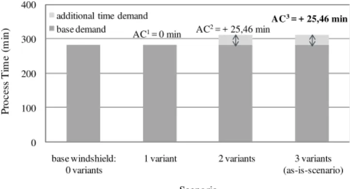
The main process ‘internal supply’ of windshields consists of the sub-processes ‘remove from internal stock’, ‘transport to sequencing area’, ‘sequencing’, and ‘transport to final assembly’, where windshields are provided part heterogeneously. The average rate of assembly X is 748 vehicles per day. As windshields are compulsory variants, 748 windshields are needed every day, which have to pass through all processes of ‘internal supply’. Comparing the existing variety of three variants to a scenario of zero windshield variants, additional process times become necessary for more frequent removals and transports because each variant has to be handled separately. Depending on the level of product variety, step-fix process times and resource demands occur, which are determined with process equations stated in (7) and displayed in Fig. 5.
Additionally to the abbreviations in the previous chapter, the authors define the inbound process time for a scenario of v variants Tv, the transport time ttv [min/container], the loading time tuv [min/container], and the sequencing time tsv [min/part] with V=3; v = 0,…,3 respectively. Further, the amount of containers V
v
b [container/day], the number of parts per container f [parts/container] and the amount of parts of variant v under product variety V are defined as V
v x
[parts/day]. Note thatX x v V
v V
v
0 .min 04 . 311 3 / 3 / 3 / 3 / min 12 . 283 3 / 3 3 3 3 3 3 3 2 2 3 2 2 3 1 1 3 1 1 3 0 0 3 0 0 3 0 0 0 0 0 0 0 X ts b tu b tt b tu b tt b tu b tt b tu b tt T X ts b tu b tt T v v (7)
0 100 200 300 400
base windshield: 0 variants
1 variant 2 variants 3 variants (as-is-scenario)
P
ro
ces
s T
im
e
(m
in
)
Scena rio
additional time demand
base demand AC1= 0 min AC2= + 25,46 min
AC3= + 25,46 min
Fig. 5. Inbound Process Times for Windshields
The cost rate of the capacity supply of personnel CRP is calculated by dividing the overall personnel costs in the period by the practical capacity supply in this period, i.e. the time that personnel is available after deductions to CRP = 0.35 EUR/min. Capacity cost rates for equipment CRE (e.g. means of transportation) are calculated accordingly and amount to CRP = 0.1 EUR/min. Altogether, variety-driven personnel complexity costs CCP3 and work equipment complexity costs CCE3 in the existing logistics systems having 3 variants, amount to 3119 Euro per year. These complexity costs are calculated with w = 250 working days per year according to (8):
. . 698
. . 2421
3 3
3 3
a p EUR w
CRE AC
CCE
a p EUR w
CRP AC
CCP
(8)
C. Inventory and Space Complexity Costs
All windshield variants have to be stocked. To ensure availability, a service level of 99.9 percent is achieved leading to z = 3.08. As for windshields purchasing costs e for variant v do not vary with the degree of product variety V, the inventory cost equations are simplified as shown in (9). The mean demand of variant v in a scenario of V variants per unit of time and the corresponding demand standard variation V
v
and V
v
respectively are given in parts per day. Inventory equations are constructed and inventory costs CIv and inventory complexity costs CCIv are calculated with r = 9 %; 0
0
= 748; 3 0
= 321; 3 1
= 104; 3 2
= 227; 3 3
= 95; 0 0
= 0; 3 0
= 25.7; 3 1
= 8.32; 3 2
= 18.2;
3 3
= 7.62; e1 = 44 EUR/part; e2 = 56.79 EUR/part; e3 = 61.41 EUR/part. Hence, CI0 = 2962 EUR per year and CI3 = 4208 EUR per year.
) (
0 0
0
0 e r e r
CI V
v v
V v
v
(9)
. . 1246
0 3
3 CI CI EUR pa
CCI (10)
Comparing the inventory on stock in the three-variants-scenario to the zero-variant-three-variants-scenario leads to an inventory increase by 25 percent. Due to higher purchasing prices for variants, inventory complexity costs amount to 1246 Euro per year (10). This represents an increase of 42 percent. Fig. 6 graphically shows this cost jump. Besides the stock of
inventory, inventory complexity costs for WIP have to be considered. WIP inventory accumulates in the sequencing area, during transport and at the assembly line. Complexity costs for WIP amount to 1080 Euro per year. In total, variety-driven inventory complexity costs CCI3 sum up to 2326 Euro per year.
0 1000 2000 3000 4000 5000
base windshield: 0 variants
1 variant 2 variants 3 variants (as-is-scenario)
Inve
nt
ory Cos
ts
(E
U
R
)
Scenario inventory complexity costs (CC) ba se inventory costs
+ 42% CCI1= + 91 EUR
CCI2= + 762 EUR
CCI3= + 1246 EUR (CCI)
Fig. 6. Inventory Complexity Costs for Windshields
In addition to process and inventory equations, floor space equations are constructed. The available floor space is clustered in internal areas (internal warehouse, assembly line and preparation area) and external areas (external warehouse). Floor space dedicated to windshields becomes necessary at different stages at the factory premises: at the warehouse, at the sequencing area and at the assembly line. Floor space costs are based on a floor space capacity cost rate per cluster in terms of monthly lease costs in EUR/m². Fig. 7 graphically illustrates the floor space equations in (11) for the sequencing area. Windshields in the sequencing area are provided with two containers per variant which leads to a linearly increasing space demand subject to the number of variants. To calculate the floor space, the container width is wc = 1.8 m², the container length is lc = 1.2 m², and the number of containers 0
0
c is 2 in all variant scenarios.
2 3
3 3 2 3 1 3 0 3
2 0
0 0
01 . 19 ) )( (
75 . 4 ) (
m l
w c c c c F
m l
w c F
c c Sequencing
c c Sequencing
(11)
The additional capacity demand of floor space AF3 in the sequencing area for 3 variants is quantified with AF3 = F3 – F0 = 14.3 m².
0 5 10 15 20 25
base windshield: 0 variants
1 variants 2 variants 3 variant (as-is-scenario)
Fl
o
o
r Sp
a
c
e
(m
²)
Va ria nt Scena rio additional floor space demand (AF) basis floor space demand
AF1= + 4,74 m²
AF2= + 9,5 m²
AF3= + 14,3 m²
With a floor space cost rate CRF of 4 EUR/m² for the sequencing area, the variety-driven floor space complexity costs at the sequencing area CCF3 are calculated in (12):
month EUR CRF
AF
CCFSequencing3 3 57 / (12)
Space complexity costs for the warehouse and the assembly line are calculated in the same way and amount to 9.50 Euro per month for the warehouse and 0 Euro per month for the assembly line. The latter can be explained, because the sequenced provision of windshields at the assembly line does not require more space than a homogenous provision in a zero-variant-scenario; both require two containers at the assembly line. Summing up, space complexity costs CCF3 amount to 798 Euro per year.
D. Overall Complexity Costs
In total, all product variety-driven complexity costs for windshields due to the existence of three variants CC3 are calculated by summing up all resource’s complexity costs (13). The overall complexity costs amount to 6248 Euro per year, which is an increase by 39 percent compared to zero-variant logistics costs.
. . 6248
3 3
3 3
3 3
a p EUR
CCF CCI
CCE CCP
CC CC
R R
(13)At first glance, the amount of 6248 Euro per year does not seem high. Taking into consideration that one automobile consists of approximately 3000 different modules and 12.000 different parts, variety-driven complexity costs for one automobile are much higher. Taking further into account that the costs of 6248 EUR per year only occur in the OEM internal inbound material flow due to the existence of three variants, it can be imagined that complexity costs rise considerably if product variety is higher for other parts (as is the case for engines, bumpers, steering wheels, tires, etc.).
According to complexity costs, impacts on the logistics performance are quantified. The variety-driven additional process time of 27.92 minutes per day represents an increase of approximately ten percent compared to a zero-variant-scenario. The process time in the automotive industry as HPV (hours per vehicle) is an important figure to perform benchmarks with other OEM in the Harbour Report [41]. With a separate statement of basis and complexity ratios of HPV, a more significant benchmark could be carried out in taking product variety-induced effects into consideration.
The case study shows, that the proposed evaluation method of product variant-driven complexity is applicable in praxis. In future, a comprehensive analysis of all parts and all models at the OEM is aimed. In particular, it is of interest if the complexity cost ratio of 39 percent and the complexity throghput time of ten percent for windshields are represantative for other parts and hence a complete automobile. The case study focused product-driven complexity costs. To account for both operative (product-driven) and structural (system-(product-driven) complexity, the
influence of the logistics system requires further analysis in the future. In this case-study, system-driven complexity for instance would account for the sequencing area that is not necessary in a zero-variant-scenario.
V. SUMMARY AND CONCLUSION
Impacts of an increased product variety in the automotive industry in particular affect the field of logistics. To capture product variety-driven complexity, the logistics system has to be evaluated subject to product variety. This knowledge regarding impacts of product variety is necessary to support strategic decisions, e.g. the determination of an optimal order penetration point in the supply chain. Towards providing relevant information, the authors of this research paper gave intensive attention to influences of product variety on logistics costs and performance. The proposed evaluation method overcomes the lack of transparency in combining several evaluation methods to a variety-specific approach, underlying the concepts of zero-base and TD-ABC. As opposed to existing evaluation methods, the proposed cost allocation is not based on estimates, rather along involved processes in a variant scenario compared to a zero-variant-scenario. The following innovations in evaluating complexity have been achieved:
- Zero-Variety approach to identify base and variant parts of the automobile
- Variety-Driven ABC (VD-ABC) to capture logistics costs and impacts on the logistics performance subject to product variety
Through the differentiation of automobile parts into base and variant parts, a reference scenario with zero variants is created, which allows the comparison to variant scenarios. With VD-ABC variety-specific additional resource demands are captured. Hence, the percentage of complexity in terms of costs and performance is identified subject to product variety. In taking specific characteristics of automotive logistics systems into account, variety equations for processes, inventory and floor space have been developed. Also, demand variability is considered through inventory equations.
The case study at a German OEM shows, that the proposed evaluation method is applicable in praxis. Findings about the amount of complexity costs and performance impacts are gained which constitute 39 percent and ten percent respectively within the given scope. Nevertheless, the method’s field of application is not restricted to inbound material flows, but can easily be adjusted to other fields of logistics (e.g. distibution) or to information flow processes (e.g. planning processes within product design).
REFERENCES
[1] H. Becker, Auf Crashkurs. Automobilindustrie im globalen
Verdrängungswettbewerb. 2nd ed., Berlin: Springer, 2007, pp. 10.
[2] M. Hüttenrauch and M. Baum, Effiziente Vielfalt. Die dritte
Revolution in der Automobilindustrie. Berlin: Springer, 2008, pp. 46.
[3] L. F. Scavarda, J. Schaffer, H. Schleich, A. C. Reis, and T. C. Fernandes, “Handling Product Variety and its Effects in Automotive Production” in Proceedings of the 19th Annual POMS Conference. La Jolla, California, 2008, pp. 2.
[4] W. Kersten, K. Rall, C. M. Meyer, and J. Dalhöfer, “Complexity Management in Logistics and ETO-Supply Chains” in T. Blecker and N. Abdelkafi, Complexity management in supply chains. Concepts,
tools and methods. Berlin: E. Schmidt, 2006, p. 325.
[5] A. Calinescu, J. Efstathiou, J. Schirn, and J. Bermejo, “Applying and Assessing Two Methods for Measuring Complexity in Manufacturing” in Journal of the Operational Research Society, 1998, pp. 723.
[6] A. Braithwaite and E. Samak, “The Cost-to-Serve Method” in
International Journal of Logistics Management, vol. 9, no. 1, 1998,
pp. 76.
[7] G. Schuh, Produktkomplexität managen. Strategien - Methoden -
Tools. 2nd ed., München: Hanser, 2005, pp. 19.
[8] P. Horváth, Controlling. 11th ed., München: Vahlen, 2009.
[9] P. K. Jagersma, “The hidden cost of doing business” in Business Strategy Series, vol. 9, no. 5, 2008, pp. 238.
[10] C. M. Meyer, Integration des Komplexitätsmanagements in den
strategischen Führungsprozess der Logistik. Bern: Haupt, 2007, pp.
21.
[11] R. Kirchhof and D. Specht, Ganzheitliches Komplexitätsmanagement. Grundlagen und Methodik des Umgangs mit Komplexität im
Unternehmen. Wiesbaden: Deutscher Universitätsverlag, 2003, pp.
38.
[12] Y. Wu, G. Frizelle, and J. Efstathiou, “A study on the cost of operational complexity in customer-supplier systems” in International
Journal of Production Economics, vol. 106, 2007, pp. 218.
[13] L. D. Fredendall and T.J. Gabriel, “Manufacturing Complexity: A Quantitative Measure” in Proc. POMS Conference, Savannah, GA, 2003, pp. 2.
[14] G. Frizelle and E. Woodcock, “Measuring complexity as an aid to developing operational strategy” in International Journal of operations & Production Management, vol. 15, no. 5, 1995, pp. 26. [15] H.-C. Pfohl, Logistiksysteme. Betriebswirtschaftliche Grundlagen.
Berlin: Springer, 2010, pp. 4.
[16] W. Pfeiffer, U. Dörrie, A. Gerharz, and S. v. Götze,
„Variantenkostenrechnung“ in W. Männel, Handbuch
Kostenrechnung. Wiesbaden: Gabler, 1992, pp. 861.
[17] R. Guerreiro, B. Rodrigues, M. Villamor, and V. Elvira, “Cost-to-serve measurement and customer profitability analysis” in The
International Journal of Logistics Management, vol. 19, no. 3, 2008,
pp. 391.
[18] J. Heina, Variantenmanagement. Kosten-Nutzen-Bewertung zur
Optimierung der Variantenvielfalt. Wiesbaden: Deutscher
Universitätsverlag, 1999, pp. 56.
[19] H. Puhl, “Komplexitätsmanagement. Ein Konzept zur ganzheitlichen Erfassung, Planung und Regelung der Komplexität in Unternehmensprozessen”. Ph.D. dissertation, University of Kaiserslautern, Germany, 1999, pp. 69.
[20] R. S. Kaplan and S. R; Anderson, Time-driven activity-based costing.
A simpler and more powerful path to higher profits. 3rd ed., Boston,
MA: Harvard Business School Press, 2009, pp. 10.
[21] P. Everaert, W. Bruggeman, G. Sarens, S. R. Anderson, and Y. Levant, “Cost modeling in logistics using time-driven ABC. Experiences from a wholesaler” in International Journal of Physical Distribution & Logistics Management, vol. 38, no. 3, 2008, pp. 173. [22] R. Hentschel, W. Gross, E. Okhan, S. Kuhn, F. Brungs, C. Schwab et
al., „Baumaschinen im nationalen Hochleistungsnetzwerk rationell produzieren und kundenindividuell für den Weltmarkt montieren“ in Forschungs- und Entwicklungsbericht BAU-MO 2008. Stuttgart: Fraunhofer IPA, 2008, pp. 160.
[23] W. Gross, J. Heimel, S. Kuhn, and C. Schwab, “Towards case-based product and network configuration for complex construction machinery” in T. Blecker and K. Edwards, Innovative processes and
products for mass customization. Berlin: GITO, 2007, p. 121.
[24] J. Schaffer, „Entwicklung und Optimierung eines treiberbasierten Modells zur Bewertung varianteninduzierter Komplexitätskosten in industriellen Produktionsprozessen“ Ph.D. dissertation, Leuphana University Lüneburg, Germany, 2010, pp. 128.
[25] J. Wulfsberg and M. Schneider, „Neue Methoden zur unscharfen Erfassung variantenbedingter Kosten“ in Zeitschrift für
wirtschaftlichen Fabrikbetrieb, vol. 100, 2005, pp. 331.
[26] O. Rosenberg, „Kostensenkung durch Komplexitätsmanagement“ in K.-P. Franz and P. Kajüter, Kostenmanagement. Wertsteigerung
durch systematische Kostensteuerung. 2nd ed., Stuttgart:
Schäffer-Poeschel, 2002, pp. 225.
[27] F. Bohne, Komplexitätskostenmanagement in der Automobilindustrie.
Identifizierung und Gestaltung vielfaltsinduzierter Kosten.
Wiesbaden: Deutscher Universitätsverlag, 1998, pp. 146.
[28] R. Lackes, „Die Kostenträgerrechnung unter Berücksichtigung der Variantenvielfalt und der Forderung nach Kostenbegleitender Kalkulation“ in ZfB Zeitschrift für Betriebswirtschaft, vol. 61, no. 1, 1991, pp. 87.
[29] K. Turner and G. Williams, “Modelling complexity in the automotive industry supply chain” in Journal of Manufacturing Technology
Management, vol. 16, no. 4, 2005, pp. 448.
[30] K. F. Pil and M. Holweg, “Linking Product Variety to Order-Fulfillment Strategies” in Interfaces, vol. 34, no. 5, 2004, pp. 395. [31] M. Toth, Eine Methodik für das kollaborative Bedarfs- und
Kapazitätsmanagement in Engpasssituationen. Ein ganzheitlicher Ansatz zur Identifikation, Anwendung und Bewertung von
Engpassstrategien am Beispiel der Automobilindustrie. Dortmund:
Verlag Praxiswissen, 2008, p. 82.
[32] A. Kuhn and B. Hellingrath, Supply Chain Management. Optimierte
Zusammenarbeit in der Wertschöpfungskette. Berlin: Springer, 2002,
p. 217.
[33] P. Nyhuis, “Produktionskennlinien – Grundlagen und
Anwendungsmoeglichkeiten” in P. Nyhuis, Beiträge zu einer Theorie der Logistik. Berlin: Springer, 2008, pp.186.
[34] M. Holweg and A. Reichhart, “Build-to-Order: Impacts, Trends and Open Issues” in G. Parry and A. Graves, Build To Order. The Road to
the 5-Day Car. London: Springer, 2008, pp. 45.
[35] D. Simchi-Levi and P. Kaminsky, Managing the supply chain. The
definitive guide for the business professional. New York:
McGraw-Hill, 2004, p. 64.
[36] A. Lechner, B. Hellingrath, and A. Wagenitz, “Evaluation of variant-driven complexity in the automotive industry: Analysis of influencing variables of product variety regarding logistics processes and structures” in J. S. Arlbjørn, Logistics and Supply Chain Management
in a Globalised Economy. Proceedings of the 22nd Annual NOFOMA
Conference, Kolding, Denmark, 2010, pp.377.
[37] S. Axsäter, Inventory control. 2nd ed., New York, NY: Springer, 2006, pp. 114.
[38] T. Gudehus and H. Kotzab, Comprehensive Logistics. Berlin: Springer, 2009, p. 296.
[39] L. Herold, Kundenorientierte Prozesssteuerung in der
Automobilindustrie. Die Rolle von Logistik und Logistikcontrolling im
Prozess vom Kunden bis zum Kunden. Wiesbaden: Deutscher
Universitätsverlag, 2005, pp. 167.
[40] H. Schleich, E. Lindemann, J. Miemczyk, G. Stone, M. Holweg, Klingebiel, K. et al., „State of the art of complexity management”, Information Societies Technology (IST) and (NMP) joint programme ILIPT, Lüneburg, Dortmund , 2005, pp. 75.