1
Evaluating the Impact of Conditional Cash Transfers on Schooling in
Honduras: An experimental approach
Paul Glewwe (University of Minnesota) Pedro Olinto (IFPRI-FCND)
Priscila Z. de Souza (EPGE-FGV)
First Draft (Incomplete)
3
I. Introduction
The Programa de Asignacion Familiar (PRAF) is one of the largest government social welfare programs in Honduras, the third poorest country in Latin America and the Caribbean (in terms of per capita GNP). PRAF was initiated in 1990 as a social safety net to compensate the poor for lost purchasing power brought about by macroeconomic adjustment. It was restructured in 1998, and now includes a reformulated project known as PRAF/IDB - Phase II (henceforth referred to as PRAF II). The objective of this project is to encourage poor households to invest in their family's education and health by
providing incentives to increase primary school enrollment, the use of preventive health care services, and the quality of both education and health-care services.
An unusual and important feature of the PRAF II project is that it includes a monitoring and evaluation component managed by the International Food Policy Research Institute (IFPRI) to assess the program’s impact over time. This paper is the first draft of a study that will evaluate the impact of PRAF II on education outcomes in poor communities in Honduras.
This paper has the following outline. The next section explains the PRAF II program and the data that have been collected so far. Section III provides some descriptive statistics from data collected in 2000 from 70 poor municipalities in Honduras. An analysis of the of the impact of the program on school attainment is presented in Section IV. Finally, Section V provides brief concluding remarks.
II. Description of PRAF II and Data
Honduras's Family Allowances Program (PRAF) began operation in 1990. The program was initially intended to be a temporary program to ease the burden of
macroeconomic adjustment on poor households. PRAF was originally a cash transfer program, distributing cash grants from health centers and schools. Continued widespread poverty in Honduras extended the time horizon of PRAF beyond the initial
4
families, so the program was modified to provide assistance that would enable those families to increase their human capital, particularly the health and education of children in poor families.
A. The PRAF II Program
In 1998, the Honduran government modified PRAF to redirect it toward these new objectives. This modified program will be referred to as PRAF II in the rest of this paper. PRAF II has the following specific objectives: (i) boost the demand for education services; (ii) encourage the “education community” to take part in children's learning development; (iii) instruct mothers in feeding and hygiene practices; (iv) ensure that sufficient money is available for a proper diet; (v) promote demand for, and access to, health services for pregnant women, nursing mothers and children under age 3; and (vi) ensure timely and suitable health care for PRAF beneficiaries. More generally, the objective of PRAF II is to increase the health and education of Honduran children in poor rural communities.
PRAF II has the following distinctive features: (i) a new system for selecting beneficiaries; (ii) interventions to stimulate the demand for and the supply of education, nutrition and health services; (iii) baseline data collection and subsequent annual data collection to measure outcomes and progress under the program; (iv) assessment of the program based on randomized treatment and control groups. PRAF II is being piloted in 70 of the poorest municipalities in Honduras. The municipalities were selected in October, 1999, and the interventions began in 2000.
To estimate the impacts of both the supply side and the demand side
interventions, IFPRI designed an evaluation procedure in which the 70 municipalities were assigned randomly to four different groups, designated as G1 – G4:
G1 = Demand side intervention only (20 municipalities)
G2 = Demand and supply side interventions (20 municipalities) G3 = Supply side intervention only (10 municipalities)
G4 = Control group without intervention (20 municipalities).
5
In each municipality in groups G1-G3, both health and education projects are implemented. Both health and education interventions take two distinct forms: a) demand side incentives (cash transfers) conditioned on school attendance and frequent heath clinic visits by the recipient; and b) supply side investments, aimed at improving the quality of schooling and health services supplied in poor rural areas. On the health side, the demand side consists of monetary transfers to pregnant women and to mothers of children under three years of age. The voucher is provided only for women who have visited health clinics every month as required by the program. Each family may receive up to three health vouchers per month, each worth approximately US$4.
The supply side of the health component consists of monetary transfers to primary health care teams, which is formed by members of the community and local health care workers (nurses and doctors when available). To receive the transfers, each team needs to prepare a plan with specific tasks and a budget specifying what equipment and medicine will be purchased for the health center. Each team receives in average US$6,000 per year, but the amount varies between US$3,000 and US$15,000, depending on the size of the population served by the health center.
To promote education, the demand incentive is generated using monetary payments that are received only if children age 6-12 enrolled in the first four years of primary school are actually attending school. A maximum of up to three children per family are eligible. Each receive approximately US$5 per month; therefore a maximum of US$15 per month is given to families. To be eligible, children need to be enrolled in school by the end of March, and need to maintain an attendance rate of 85%.
The supply side intervention is payments to Parent Teacher Associations
organized around each primary school. The associations need to obtain legal status, and need to prepare plans to improve the quality of the education provided by their respective schools. The plan needs to include a budget for the list of equipment and materials
6
B. Data
After the 70 poor municipalities were chosen, baseline data were collected from all 70 before the PRAF II program was implemented in the municipalities in groups G1, G2 and G3. The baseline data were collected in 2000 from August to
mid-December. The follow up survey was conducted in 2002, from mid May to mid-August. From each municipality, eight communities (“clusters”) were randomly selected, and from each cluster 10 dwellings were randomly selected. Assuming one household per dwelling, this implies a total baseline sample of 5600 households. In fact, some of these dwellings had more than one household, so the total number of households selected in the baseline was 5784. In most cases, each group of 10 dwellings is found within a different village (aldea) of the municipality, but in some cases two or more groups of 10 are from the same village. These 5784 households contained a total of 30,588 members.
In the follow up 2002 survey, an attempt was made to interview households that moved away from where they were first interviewed in 2000. Also, new households derived from original baseline households were interviewed whenever they contained members that were in the initial survey and who belonged to the program’s targeted population (pregnant women, lactating mothers and children 0-16). As seen in table 7, approximately 84% of the households interviewed in 2000 were interviewed again in 2002, and approximately 3.6% of the original households spun off at least one new household. These figures are very similar across the four treatment groups. Therefore, we do not expect severe attrition bias in our impact estimates below.
Three kinds of data were collected. First, a household questionnaire was administered to all households from August to December, 2000. That questionnaire collected data on: a) housing; education and employment of all household members; b) education (very detailed) of all children age 6-16; c) the health of all women who were pregnant in the past 12 months; d) the health of all children below three years of age (and height, weight and hemoglobin information for all children under five years); e)
7
age 6-12 doing various activities; and k) households’ evaluation of the quality of local health centers and primary schools.
Second, data were collected on community characteristics in each of the 560 clusters. The data include: a) whether the community has a primary school, a public hospital or public transport; b) daily wage rates for local agricultural and non-agricultural work; c) the availability of work away from the community; d) a small amount of
information on local crime; and e) prices for a large number of food items and the going daily wage rate.
Third, questionnaires were administered to primary schools in each of the 70 municipalities. Three schools were randomly selected from each municipality, totaling 210 schools. The school questionnaire collected the following data: a) general
information on the school (days open, number of grades, etc.); b) characteristics of teachers; c) pedagogical aids (library books, dictionaries, paper etc.); and d) school organizations (PTA, teachers association, etc.).
III. Education Outcomes from the 2000 Baseline Data
This section presents some basic data on the education outcomes of children of primary school age, age 6-12. This is done to set the stage for the analysis in Section IV of the impact of the program on years of schooling for children in this age group.
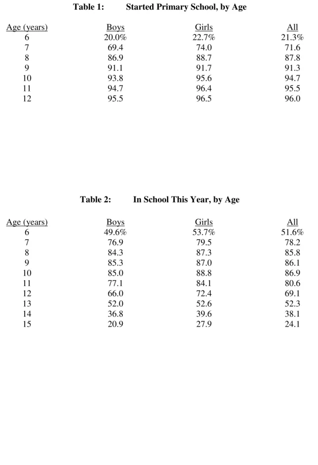
Table 1 shows the ages by which children of different ages have started primary school. Although the official policy of Honduras’ Ministry of Education is that children should begin school at age 6, only 21% of 6-year-old children from these 70 poor municipalities have started schooling by that age. Yet by the time they are seven years old, most children have started primary school; 72% have done so by that age. By age 10, 95% of these children have started primary school, and this percentage peaks at about 96% at age 12. Thus only about 4% of the children in these poor municipalities never attend school, but delayed enrollment in primary is a common phenomenon. The table also provides this figures by sex; girls are slightly more likely to start on time, but the difference is not very large.
8
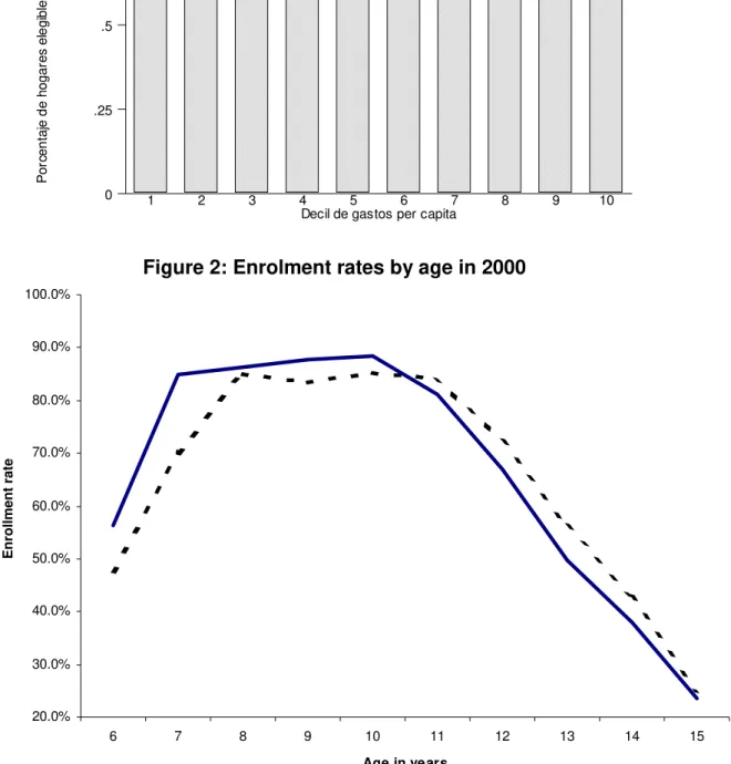
these 70 municipalities, enrollment peaks at 86-87% at ages 8-10, after which it steadily declines so that only about 15% of 16-year-olds are enrolled in school. (Note, ages 6 and 7 include some children who are still enrolled in pre-school..) Even by age 13 only about half of these children are still enrolled in school. Girls are more likely to be enrolled in school at all ages, but the difference is not very large.
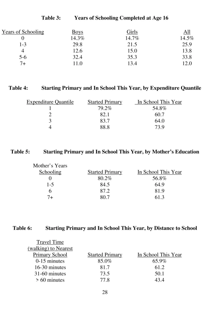
The tables examined so far show that almost all (95%) of Hondurans children in these poor municipalities do enroll in primary school, yet they often start their schooling 1-2 years late and they do not stay in school very long. In particular, about half have dropped out by age 13 and about 85% have dropped out by age 16. This implies that these children complete only a few years of schooling before leaving school. This is shown in Table 3, which shows years of schooling completed for children who are 16 years old. About 15% have completed a single year of primary school, and about one fourth completed only 1-3 years of schooling. A common rule of thumb is that four or more years of schooling are needed before someone acquires and retains basic literacy skills, which implies that about 40% of the children in these communities will be illiterate when they become adults. About half (48%) attain 4-6 years of schooling, and only 12% attain seven or more years (i.e. secondary school). Clearly, school attainment in these Honduran communities is quite low and fully justifies programs to increase it.
The next three tables examine patterns that may explain why children are not enrolled in school. Table 4 examines, for children age 6-16, whether children have started primary school and whether they are currently enrolled in school, by income levels. More precisely, children were divided into four groups of equal size according to household consumption expenditures per capita. The poorest 25% are called quartile 1, the next poorest 25% are quartile 2, and so on. For the poorest quartile, only 79% have started primary school and only 55% are currently enrolled in school. These numbers increase steadily for wealthier groups, until at the fourth quartile (wealthiest 25%) 89% of these children have started primary school and 74% are still in school. This suggests, as one would expect, that better off households are more likely to enroll their children in school.
9
looks at starting primary school and current school attendance when children are classified according to their mothers’ level of education. About one third (36%) of children age 6-16 have mothers with no education at all. About 80% of those children had started primary school, and only 57% were currently attending school. Children whose mothers had some primary school education (1-5 years) fared better; 85% had started primary school and 65% were currently attending school. Children whose mothers had completed primary schooling (about 12% of the sample) performed best of all, with 87% starting primary school and 82% currently in school. Somewhat
surprisingly, the small number of children whose mothers report higher than primary education (0.4% of the sample) did not do as well as mothers who had some or complete primary education; this could reflect the small sample size or it may simple indicate that these women were misclassified.
Another potentially important determinant of school progress is the distance to the nearest primary school. All households were asked how long it would take them to walk to the primary school that is nearest to their homes. Two thirds (68%) of the children live in households where this travel time (one way) is 15 minutes or less. About one fourth (23%) live in households were the travel time is 16-30 minutes, while another 6% have travel times of 31-60 minutes and 2% report travel times of more than one hour (the largest was five hours). Table 6 examines the relationship between travel time, starting primary school and current school attendance. About 85% of children who live within 15 minutes of a primary school have started primary school. This figures drops to 82% for children with travel times of 16-30 minutes and 74% for children with times of 31-60 minutes, and then increases slightly to 78% for children with times exceeding one hour. Current school enrollment has a clear monotonic relationship, ranging from 66% for children within 15 minutes of a primary school to 43% for children whose travel times exceed one hour.
IV. Empirical Methods: Estimating the impact of PRAF II on Schooling
The central problem in the evaluation of any social program is the fact that households participating in the program cannot be simultaneously observed in the
10
or household in the treated state (i.e., during or after participation in the program) and Y0
is the outcome in the untreated state (i.e., without participating in the program). Then the gain for any given individual or household from being treated by the program is
) (Y1−Y0
=
∆ . However, at any time a person is either in the treated state, in which case Y1 is observed and Y0 is not observed, or in the untreated state, in which case Y1 is
unobserved and Y0 is observed. Given that missing Y1 or Y0 preclude measurement of this
gain for any given individual, one has to resort to statistical methods as a means of addressing this problem (e.g., see Heckman, LaLonde and Smith, 1999). The statistical approach to this problem replaces the missing data on persons using group means or other group statistics, such as medians.
For example, the majority of the studies on evaluation of social programs focus on the question of whether the program changes the mean value of an outcome variable among participants compared to what they would have experienced if they had not participated. The answer to this question is summarized by one parameter called the “the mean direct effect of treatment on the treated.” Using formal notation, the mean effect (denoted by the expectation operator E) of treatment on the treated (denoted by T=1) with characteristics X may be expressed as
(
T X) (
E Y Y T X) (
EY T X) (
EY T X)
E ∆| =1, = 1− 0 | =1, = 1| =1, − 0 | =1, . (1)
The term E
(
Y1|T =1,X)
can be reliably estimated from the experience of program participants. What is missing is the mean counterfactual term E(
Y0 |T =1,X)
that summarizes what participants would have experienced had they not participated in the program.The variety of solutions to the evaluation problem differ in the method and data used to construct the mean counterfactual term E
(
Y0 |T =1,X)
. For example, one11
experimentation or randomization of individuals into treatment and control groups. Experimental designs use information from individuals or households in the control group to construct an estimate of what participants would have experienced had they not participated in the program, i.e., the term E
(
Y0 |T =1,X)
.1The empirical framework adopted by the PRAF II administration for the purposes of evaluating the program’s impact offers a very flexible approach to solving the
evaluation problem. Its advantages are derived from two key features. Firstly, it is an experimental design with randomization of municipalities, rather than households or individuals, into treatment and control groups.2 Secondly, data are collected from all households in both treated and control localities before and after the start the treatment. The combination of these two features permit researchers to evaluate the “mean direct effect of treatment on the treated” or in other words the impact of the program on program participants using any of the estimators available in the evaluation literature, including the before-after estimator, the difference-in-differences estimator, and the fist-difference or (cross-sectional) estimator discussed in more detail below.
Given the experimental design one may then construct all of the estimators commonly used in program evaluation. These are:
i) the cross-sectional difference estimator (CSDIF) that compares differences in the means of the outcome variable Y between groups A and B during the periods after the implementation of the program (i.e., t=1,2,3,…)
( )
(
)
[
| =1, =1]
−[
(
( )
| =0, =1)
]
= EY t T E E Y t T ECSDIF for t=1,2,3,… (2)
and,
1 For a more thorough discussion of the various solutions to the evaluation problem see Heckman, LaLonde, and Smith (1999).
2
12
ii) the double differences or difference-in-differences estimator (2DIF) that measures program impact by comparing differences in the means of the outcome between group A and B in post survey rounds with the differences in the mean the means of the outcome between group A and B in the pre –program round. Formally,
(
)
(
)
[
]
[
(
(
)
)
]
(
)
(
)
[
0 | 1, 1]
[
(
(
0)
| 0, 1)
]
. 1 , 0 | 1 1 , 1 | 1 2 = = = − = = = − = = = − = = = = E T t Y E E T t Y E E T t Y E E T t Y E DIF (4)Each of these estimators has some advantages and shortcomings associated with it. However, the 2DIF estimator in comparison to the CSDIF estimators is the preferred estimator for program evaluation. For example, one major advantage of the 2DIF estimator over CSDIF in evaluating the mean direct effect of treatment on the treated is that the former controls for any pre-existing differences in the expected value of Y between households in treatment and control localities. Measuring program impact based exclusively on post-program difference in the mean level of the outcome indicator between treatment and control localities, as done by the first difference estimator, may lead to potentially misleading conclusions about program impact.
Ultimately, the extent to which the CSDIF estimator may lead to biased results depends critically on whether the selection of treatment and control localities was indeed random. Pure and proper randomization of the selection of localities would ensure that there are no significant pre-program differences in the outcome variable of interest between treatment and control localities, i.e.,
(
)
(
)
[
EY t =0 |T =1,E=1]
=[
E(
Y(
t=0)
|T =0,E=1)
]
. (6)Satisfaction of condition (5) also ensures that CSDIF=2DIF. In other words,
randomization implies that focusing exclusively on post-program comparisons between treatment and controls yields unbiased conclusions about the impact of the program.
13
For most of the key outcome indicators of interest such as school enrollment and attendance, data are available before and after the start of the program that permit implementation of the 2DIF estimator. For some indicators, however, such as such as school desertion and labor force participation, observations in the baseline were affected by severe seasonality due to the coffee harvest that starts in October and November. For these outcome indicators, the CSDIF estimator provides the best available option for evaluating PRAF II.
Program Evaluation Within the Regression Framework
The discussion so far focused on evaluating PRAF II without making any adjustments for the role of observed characteristics of the individual, the household and the locality on the variation in the observed value of the outcome indicator of interest. Without any adjustment for the role of such confounding factors all the differences in the mean value of the outcome indicator are attributed to the program. As a matter of
principle it is preferable to have an estimate of the impact of the program net of the influence of these observed characteristics on the difference in the mean value between treatment and control households.
We also assume that the objective of the regression analysis is to obtain a consistent and unbiased estimate of the effect of the program on households or
individuals eligible for the program. WE do not address the issue of take up, although to the extent that take up differs a lot from eligibility biases from selectivity may be at work.
We begin with the case where there are data available for treatment and control households before and after the start of the program.3 Restricting the sample to eligible households only, the various estimators for program evaluation discussed above that
3
We assume only one observation after the start of the program for expositional simplicity only. More than one round of observations after the start of the program can be easily accommodated by including an additional binary variable (say R3) along its
14
control for individual, household and locality observed characteristics can be obtained by estimating a regressions equation of the form
( )
i t T( )
i R T( )
i R X(
i v t)
Y , =α +βT +βR 2+βTR( * 2)+
å
jθj j +η , , , (7)where Y(i,t) denotes the value of the outcome indicator in household (or individual) i in period t, α, β, γ and θ are fixed parameters to be estimated, T(i) is an binary variable taking the value of 1 if the household belongs in a treatment community and 0 otherwise (i.e., for control communities), R2 is a binary variable equal to 1 for the second round of the panel (or the round after the initiation of the program) and equal to 0 for the first round (the round before the initiation of the program), X is a vector of household (and possibly village) characteristics and η is an error term summarizing the influence random disturbances.
To better understand the preceding specification it is best to divide the parameters into two groups: one group summarizing differences in the conditional mean of the outcome indicator before the start of the program (i.e., α, βT,) and another group
summarizing differences after the start of the program (i.e., βR, and βTR). Specifically,
the coefficient βT allows the conditional mean of the outcome indicator to differ between
eligible households in treatment and control localities before the initiation of the program whereas the rest of the parameters allow the passage of time to have a different effect on households in treatment and control localities. For example, the combination of
parameters βR andβTR allow the differences between eligible households in treatment
and control localities to be different after the start of the program.
One advantage of this specification is that the t-values associated with some of these parameters provide direct tests of a number of interesting hypotheses. For example, the t-value associated with the estimated value βT provides a direct test of the equality in
15
conditional mean of the outcome indicator should be the identical across treatment and control households/individuals.
Specifically, given the preceding specification, the conditional mean values of the outcome indicator for treatment and control groups before and after the start of the program are as follows:
(
)
[
EY|T =1,R2=1,X]
=α+βT +βR +βTR +å
jθjXj (8a)(
)
[
EY|T =1,R2=0,X]
=α+βT +å
jθjXj (8b)(
)
[
EY|T =0,R2=1,X]
=α+βR +å
jθjXj (8c)(
)
[
EY|T =0,R2=0,X]
=α+å
jθjXj (8d)According to the preceding specification, the cross-sectional difference estimator is given by the expression:
= −
= (a c)
CSDIF
(
) (
)
[
EY |T =1,R2=1,X −E Y |T =0,R2=1,X]
= β +T βTR. (9)while the before-and-after difference estimator is given by
= −
= (a b)
BADIF
(
) (
)
[
EY |T =1,R2=1,X −EY |T =1,R2=0,X]
= β +R βTR. (10)Expression (9) describing the CSDIF estimator highlights the fact that the estimated impact of the program is inclusive of any pre-program differences between treatment and control groups (summarized by the presence of the βT term). Along
16
or aggregate effects in the changes of the outcome indicator Y (summarized by the presence of the βR term).
The advantage offered by the difference in differences (2DIF) estimator is that it provides an estimate of the impact of the program that is net of any pre-program
differences between treatment and control households and/or any time trends or aggregate effects in changes of the values of the outcome indicator.4 By comparing before and after differences between treatment and control households (or differences between treatment and control households after and before the program) one is able to get an estimate of the impact of the program (summarized by the single parameterβTR).
TR
d b c a d c b a
DIF = ( − )−( − ) =( − )−( − ) = β
2 (11)
Using the terminology of Heckman et al. (1999), the parameterβTR provides an
estimate of the “mean direct effect of treatment on those who take the treatment.” It should also be noted the program effect summarized by the parameterβTR is inclusive of
the role that the operational efficiency or inefficiency with which the program operates. It is likely that persistent delays in the processing of forms in some municipalities and other administrative bottlenecks may lead to weaker impacts of the program on households residing in these municipalities relative to that in municipalities where the program is operating more efficiently.
In this paper, the vector X typically consists of variables characterizing the age and gender, and grade in which students currently attend.. Given that the vector X does not contain any supply-related variables, βTR is an estimate of the impact of the
conditional cash transfers (demand-side effects) and the improvements in the quantity and quality (or supply-side effects) of educational and health services and facilities associated with the PRAF II program.
4
17
Estimating Longer-Term Impact: A Markov Schooling Transition Model
There are many schooling indicators that can be affected by the program, including effects on the initial age of school entry, dropout rates, grade repetition rates and the rate of school reentry among dropouts. To analyze the experimental program impact along these various dimensions, we adopt a Markov schooling transition model. This transition model provides a convenient framework to study the long-term impact of program participation on school attainment.
Let fg,a be the proportion of children of age a enrolled in grade g, fne,a the
proportion of children of age a never enrolled and fdrop,a the proportion of children of age
a that were enrolled at school in the past, but dropped out. For six-year-old children, there
are three possible schooling states (not yet enrolled, enrolled in grade one, or enrolled in grade 2) with the majority of six-year-olds enrolled in grade one. For seven-year-old children, there are six possible schooling states (not yet enrolled, dropped out after being enrolled as a six-year-old, enrolled in grade one, enrolled in grade 2, and enrolled in grade three) with the majority of seven-year-olds enrolled in grade two.
At age a, the probability of moving from state i to state j is given by pij,a.
Therefore, the transition from age 6 to 7 is given by:
÷ ÷ ÷ ø ö ç ç ç è æ ú ú ú ú ú ú û ù ê ê ê ê ê ê ë é = ÷ ÷ ÷ ÷ ÷ ÷ ø ö ç ç ç ç ç ç è æ 6 , 6 , 1 6 , 2 6 , 53 6 , 42 6 , 41 6 , 33 6 , 32 6 , 23 6 , 22 6 , 21 6 , 13 6 , 12 6 , 11 7 , 7 , 7 , 1 7 , 2 7 , 3 0 0 0 0 ne ne drop f f f p p p p p p p p p p p f f f f f
where the cells set equal to zero impose the restrictions that students cannot regress in grades and once enrolled, they can no longer enter the state of being “never enrolled”.
Thus, we denote the transition rule from age a to age a+1 by fa+1=Aafa. To
simulate the impacts of the program for a synthetic cohort from data on a short panel we require two assumptions:
18
ii) The transition matrices for an age group do not change over time.
Let sa be the schooling level at age a, T a variable indicating the whether the child
participates in the program and H a vector of treatment and schooling level history before age a. Formally, assumption (i) can be expressed as:
P(sa+1/sa, Ta, Ha)=P(s a+1/sa, Ta)
Under assumptions (i) and (ii), and given an initial vector of state proportions at some age, the predicted schooling state distribution at a later age can be obtained by:
where a is an age later than as, and T=1 if the child participates in the program, and T=0
otherwise.
V. Empirical Results
In this section we present the empirical results obtained from applying the two methods of estimating program impact explained above. We use the 2DIF estimators for most schooling indicators. For indicators that were likely affected by seasonality during the baseline survey (i.e., the coincidence of the coffee harvest season with the survey of the control group), we adopt the CSDIF estimator for the 2002 data.
Tables A.1 to A.5 in the appendix present 2DIF estimates of impact for several outcome indicators of interest for the program’s target population, children aging 6-12. These estimates were obtained from the following regression equation:
Yit = b0 + b1.G1i + b2.G2i + b3.G3i + b4.D2002it + b5.G1i.D2002it + b6.G2i.D2002it +
19
where G1i is an indicator variable determining whether household i lives in demand side-only municipality, G2i determines whether household i lives in a demand+supply-side municipality, and G3i determines whether household I lives in a supply side-only municipality. The dummy for households living in control municipalities (G4i) is
excluded. Therefore, b0 gives the mean outcome for the control households in 2000, and b4 gives the estimated change in this mean between 2000 and 2002. b1-b3 give the average differences between the respective treatment groups (G1, G2 and G3), and the control group G4 in the baseline in 2000. The 2DIF estimates of impact for each treatment are therefore given by parameters b5-b7.
Tables A.1 to A.5 also present statistical tests for the existence of synergetic effects between supply-side and demand-side interventions. That is, we test the null hypothesis H0: b6 = b5 + b7, against the alternative Ha: b6 ≅ b5 + b7. As one can see, we cannot reject the null hypothesis at any conventional significance level, and for any of the outcome indicators. Therefore, in the rest of the paper we focus on the analysis of impact via the following regression model
Yit = c0 + c1.Di + c2.Si + c3.D2002it + c4.Di.D2002it + c5.Si.D2002it + eit, (13),
where Di indicates that the municipality was treated with demand-side interventions, and Si indicates supply-side interventions. Therefore, observations from municipalities G2 will exhibit Di=1 and Si=1, while observations from the control municipalities G4 will exhibit Di=1 and Si=1. Accordingly, G1(G3) observations will exhibit Di=1 and Si=0 (Di=0 and Si=1).
20
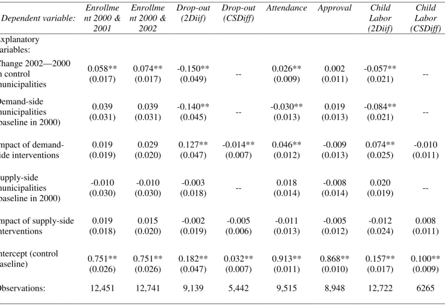
As it can be seen in table 9, there appears to be no impact of the program in enrollment rates for the 6-12 age group as a whole. This disappointing result can perhaps be explained by the graph in figure 2. The graph shows that enrollment rates for the ages 7-12, the main target of the program, are relatively high and therefore not likely to respond sharply to any demand-side cash transfers. That is, perhaps the opportunity cost of time for children aging 7-12 is still not elevated enough to permit a high response to the program. The graph shows that the program could have a greater impact if it had also targeted children aging 13-15.
Table 9 also shows strong and positive estimates of impact of the demand-side interventions on school dropouts. As discussed above, these unexpected results are likely due to the seasonality problems experienced by the baseline survey in 2000. Therefore, we shift attention to the CSDIF estimates of program impact on dropout rates. These indicate that the demand-side cash transfers have reduced dropout rates by 1.4 percentage points from a 3.2% basis, that is, a higher than 50% reduction in the rate of school
dropout.
Table 9 also presents estimates of the impact of the PRAF II on school attendance. As shown, the results point to a 4.6 percentage point increase (from an average of approximately 91%) in attendance rates due to the program’s demand-side interventions.
Therefore, while there is no evidence of increased enrollment due to the program, kids in the program appear less likely to dropout before the end of the school year and do seem to attend more classes. However, this increased contact with the school does not appear to boost school performance. As indicated in Table 9, approval rates do notseem to be higher for kids participating in program.
Finally, the impact of the program on child labor is also examined in Table 9. As seen, the 2DIF estimate suggests a 7.4 percentage point increase in the incidence of child labor up from approximately 16%. This substantial and counterintuitive result is also explained by the effect of seasonality during the baseline survey. That is, in 2000, the incidence of child labor for the control and supply-side treatment groups was
21
suggest that he program has no impact whatever in reducing the prevalence of child labor.
Estimating the schooling transition model
As observed above, there are very many channels via which the demand-side cash transfers may affect schooling. We next present the results of the estimation of the
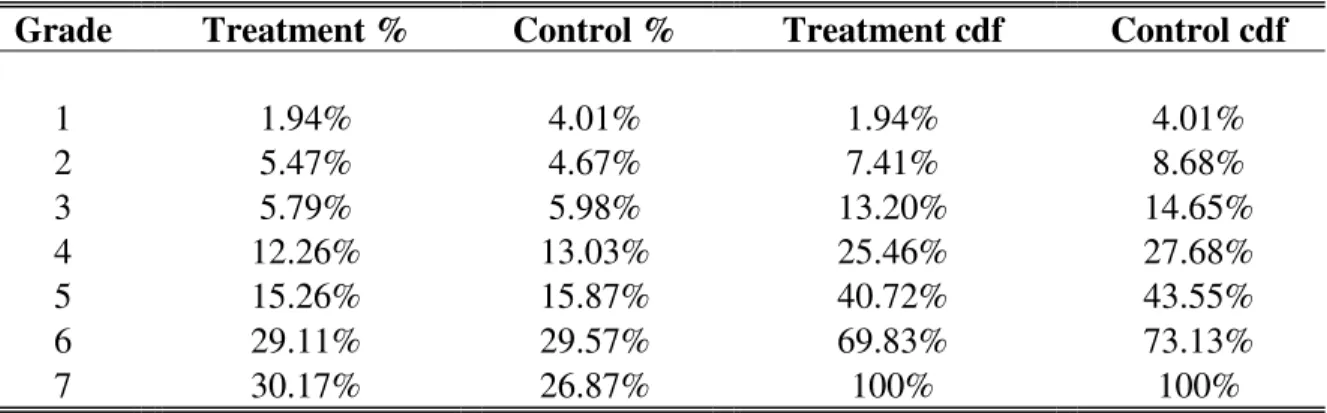
schooling transition model that was describe above, and can be used to summarize the impact of the program via several indicators into the impact of education attainment at age 13. We follow a procedure suggested in Behrman, Sengupta and Todd (2002) to estimate the probability transition matrices for ages 6 to 12, and then to simulate the resulting distribution of education attainment at age 13. The results are presented in table 18 and are graphically illustrated in figure 6.
Table 7 gives the simulated pdf and cdf values for treatments and controls, where treatment now refers to being a beneficiary of PRAF for 7 years from age 6 to 13. Figure 6 plots the corresponding histograms and cdf’s which reveal a slight difference between the treatment and control groups. Our simulation predicts an average education
attainment of 5.42 for program participants at age 13, as compared to 5.28 years for controls. A comparison of the predicted cdf for treatments and controls shows that the program induces about 12.3% more children to continue schooling into secondary school grades. These estimates can be combined with estimates of return to schooling in
Honduras to assess the cost-benefit ratio of the program.
VI. Conclusion
22
control group, where no transfers were made. Baseline data were collected from a random sample of 5,600 households living in these seventy municipalities before the program was implemented. A second round of surveys of the same families was conducted two years after the start of the program.
The results from the regression analysis and the simulated schooling transition model show a very weak impact of the demand-side component of the program, and no impact whatsoever of the supply-side interventions. The data suggest that the weak impact of the demand-side component is perhaps associated with poor targeting. Enrollment rates for children aging 6-12 were relatively high before program
implementation, thereby weakening the potential for impact. The design of the program should be revised to allow participation of older children (13-16).
23
Figura 1: Cobertura del Bono Escolar por decil de gastos per cápita.
P
or
cen
taj
e d
e hoga
res
el
e
gi
bl
es
que r
e
ci
b
io
e
l be
n
e
fic
io
Decil de gastos per capita 0
.25 .5 .75 1
Recibio su Bono Escolar
1 2 3 4 5 6 7 8 9 10
Figure 2: Enrolment rates by age in 2000
20.0% 30.0% 40.0% 50.0% 60.0% 70.0% 80.0% 90.0% 100.0%
6 7 8 9 10 11 12 13 14 15 Age in years
Enrol
lm
e
n
t ra
24
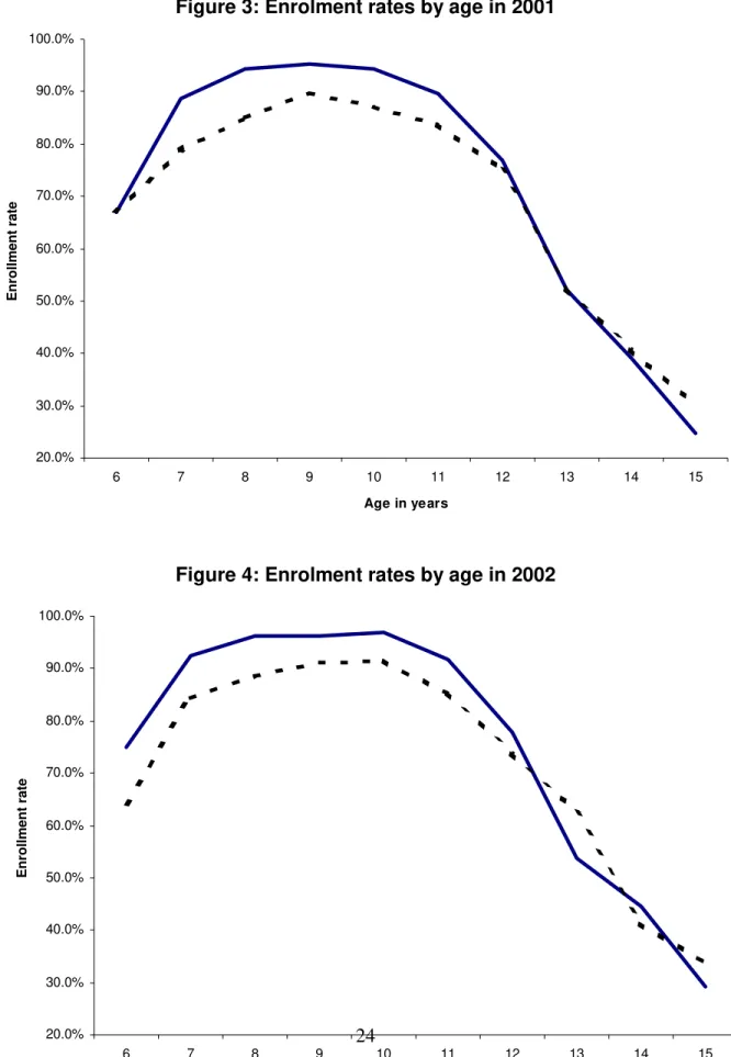
Figure 3: Enrolment rates by age in 2001
Figure 4: Enrolment rates by age in 2002
20.0% 30.0% 40.0% 50.0% 60.0% 70.0% 80.0% 90.0% 100.0%
6 7 8 9 10 11 12 13 14 15 Age in years
Enrol
lm
e
n
t ra
te
20.0% 30.0% 40.0% 50.0% 60.0% 70.0% 80.0% 90.0% 100.0%
6 7 8 9 10 11 12 13 14 15 Age in years
Enrol
lm
e
n
t ra
25
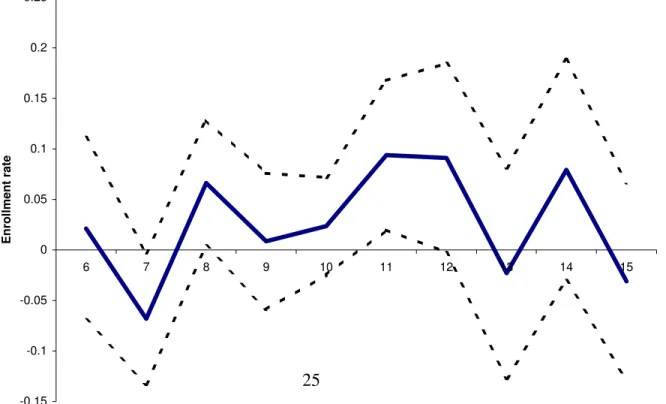
Figure 5: Average Demand Side Treatment Impacts on Enrollment by Age (2001-2000)
Figure 5: Average Demand Side Treatment Impacts on Enrollment by Age (2002-2000)
-0.25 -0.2 -0.15 -0.1 -0.05 0 0.05 0.1 0.15 0.2
6 7 8 9 10 11 12 13 14 15
Age in years
E
n
rol
lm
ent rate
-0.15 -0.1 -0.05 0 0.05 0.1 0.15 0.2 0.25
6 7 8 9 10 11 12 13 14 15
Age in years
E
n
rol
lm
e
26
Figure 6: Simulated Effects of Demand Treatment on Educational Attainment at 13
0 0.05 0.1 0.15 0.2 0.25 0.3
1 2 3 4 5 6 7
Demand treatment Control
0 0.1 0.2 0.3 0.4 0.5 0.6 0.7 0.8 0.9 1
1 2 3 4 5 6 7
27
Table 1: Started Primary School, by Age
Age (years) Boys Girls All
6 20.0% 22.7% 21.3%
7 69.4 74.0 71.6
8 86.9 88.7 87.8
9 91.1 91.7 91.3
10 93.8 95.6 94.7 11 94.7 96.4 95.5 12 95.5 96.5 96.0
Table 2: In School This Year, by Age
Age (years) Boys Girls All
6 49.6% 53.7% 51.6%
7 76.9 79.5 78.2
8 84.3 87.3 85.8
9 85.3 87.0 86.1
28
Table 3: Years of Schooling Completed at Age 16
Years of Schooling Boys Girls All
0 14.3% 14.7% 14.5%
1-3 29.8 21.5 25.9
4 12.6 15.0 13.8
5-6 32.4 35.3 33.8 7+ 11.0 13.4 12.0
Table 4: Starting Primary and In School This Year, by Expenditure Quantile
Expenditure Quantile Started Primary In School This Year
1 79.2% 54.8%
2 82.1 60.7
3 83.7 64.0
4 88.8 73.9
Table 5: Starting Primary and In School This Year, by Mother’s Education
Mother’s Years
Schooling Started Primary In School This Year
0 80.2% 56.8%
1-5 84.5 64.9
6 87.2 81.9
7+ 80.7 61.3
Table 6: Starting Primary and In School This Year, by Distance to School
Travel Time (walking) to Nearest
Primary School Started Primary In School This Year
0-15 minutes 85.0% 65.9%
16-30 minutes 81.7 61.2
31-60 minutes 73.5 50.1
30
Table 7: Sample evolution from 2000 to 2002 by random treatment group.
Grupo de asignacion aleatoria
Demanda Demanda+oferta Oferta Control Total
Ubicacion en el 2002
Hogar original 85.4% 84.5% 85.6% 82.5% 84.3%
Hogar derivado 3.9% 3.3% 3.6% 3.4% 3.6%
Murió 0.6% 0.7% 0.6% 0.8% 0.7%
Movio, no se pudo localizer 5.7% 6.0% 4.5% 7.0% 6.0%
Ignorado 0.7% 0.7% 0.9% 0.8% 0.8%
Fracaso (Rechazo/Ausente) 1.6% 2.2% 2.3% 2.5% 2.1%
Fracaso (Desocupada/No
encontrada) 2.1% 2.6% 2.5% 2.9% 2.5%
Total de personas 8823 8797 4197 8749 30566
Table 8: Coverage and leakage of the cash transfers in 2001.
Treatment Group
Demand (G1)
Demand +supply
(G2)
Supply (G3)
Control (G4)
Coverag
e 726/959 746/942
75.7% 79.2%
Leakega 15/689 12/669 3/798 19/1625 2.2% 1.8% 0.4% 1.2%
Table 9: Estimated impact of PRAF’s demand and supply side interventions on schooling indicators
Dependent variable:
Enrollme nt 2000 &
2001
Enrollme nt 2000 &
2002
Drop-out (2Diif)
Drop-out (CSDiff)
Attendance Approval Child Labor (2Diif) Child Labor (CSDiff) Explanatory variables: Change 2002—2000 in control municipalities 0.058** (0.017) 0.074** (0.017) -0.150**
(0.049) --
0.026** (0.009)
0.002 (0.011)
-0.057**
(0.021) --
Demand-side municipalities (baseline in 2000)
0.039 (0.031)
0.039 (0.031)
-0.140**
(0.045) --
-0.030** (0.013)
0.019 (0.013)
-0.084**
(0.021) --
Impact of demand-side interventions 0.019 (0.019) 0.029 (0.020) 0.127** (0.047) -0.014** (0.007) 0.046** (0.012) -0.009 (0.013) 0.074** (0.025) -0.010 (0.011) Supply-side municipalities (baseline in 2000)
-0.010 (0.030)
-0.010 (0.030)
-0.003
(0.018) --
0.018 (0.014)
-0.008 (0.014)
0.020
(0.019) --
Impact of supply-side interventions 0.019 (0.018) 0.015 (0.020) -0.002 (0.019) -0.005 (0.006) -0.011 (0.013) -0.005 (0.012) -0.012 (0.024) 0.008 (0.011) Intercept (control
baseline) 0.751** (0.026) 0.751** (0.026) 0.182** (0.047) 0.032** (0.007) 0.913** (0.011) 0.868** (0.010) 0.157** (0.017) 0.100** (0.009)
32
Table10: Impacto en la tasa de matricula escolar por edad (2001-2000)
Edad Control Doble-Diferencia
2000 2001 Cambio Demanda-Control valor-P
6 47.6% 66.8% 19.2% -8.7% 0.086
7 70.0% 78.7% 8.8% -4.9% 0.224
8 85.1% 85.2% 0.1% 8.1% 0.008
9 83.5% 89.7% 6.2% 1.4% 0.668
10 85.4% 87.3% 1.9% 3.8% 0.139
11 84.3% 83.8% -0.5% 8.8% 0.024
12 72.2% 75.0% 2.7% 7.1% 0.13
13 56.1% 52.4% -3.7% 6.2% 0.207
14 42.7% 40.7% -2.1% 3.1% 0.52
15 25.0% 29.9% 5.0% -3.7% 0.257
Table 11: Impacto en la tasa de matricula escolar por edad (2002-2000)
Edad Control Doble-Diferencia
2000 2002 Cambio Demanda-Control valor-P
6 47.6% 64.2% 16.6% 2.1% 0.642
7 70.0% 84.3% 14.4% -6.8% 0.040
8 85.1% 88.6% 3.4% 6.6% 0.037
9 83.5% 91.3% 7.7% 0.9% 0.801
10 85.4% 91.6% 6.2% 2.4% 0.334
11 84.3% 85.3% 1.1% 9.4% 0.014
12 72.2% 73.9% 1.7% 9.1% 0.056
13 56.1% 62.4% 6.3% -2.3% 0.660
14 42.7% 41.2% -1.5% 7.9% 0.153
15 25.0% 33.7% 8.8% -3.1% 0.526
33
Table12: Impacto en la deserción escolar en 2002 para grados de 1 a 6
Grado Control Demanda-Control Valor-P
1 5.3% -4.3% 0.000
2 2.6% -0.7% 0.508
3 3.0% -1.0% 0.368
4 2.3% 0.2% 0.817
5 3.6% -0.7% 0.697
6 3.3% 1.5% 0.349
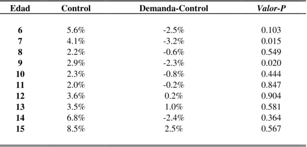
Table 13: Impacto en la deserción escolar en 2002 por edad
Edad Control Demanda-Control Valor-P
6 5.6% -2.5% 0.103
7 4.1% -3.2% 0.015
8 2.2% -0.6% 0.549
9 2.9% -2.3% 0.020
10 2.3% -0.8% 0.444
11 2.0% -0.2% 0.847
12 3.6% 0.2% 0.904
13 3.5% 1.0% 0.581
14 6.8% -2.4% 0.364
15 8.5% 2.5% 0.567
Table 14: Impacto en la tasa de asistencia escolar por grado de la primaria
Grado Control Doble-Diferencia
2000 2002 Cambio Demanda-Control valor-P
1 88.8% 93.4% 4.7% 3.0% 0.145
2 91.4% 93.4% 2.0% 6.5% 0.002
3 90.5% 94.3% 3.8% 3.9% 0.033
4 93.5% 94.1% 0.6% 6.2% 0.000
5 93.2% 95.3% 2.1% 3.3% 0.049
6 93.9% 95.4% 1.5% 2.7% 0.107
34
Table 15: Impacto en la tasa de asistencia escolar por edad
Edad Control Doble-Diferencia
2000 2002 Cambio Demanda-Control valor-P
6 90.6% 93.3% 2.7% 4.2% 0.040
7 90.8% 93.3% 2.4% 5.6% 0.010
8 91.7% 94.2% 2.5% 5.0% 0.012
9 91.4% 94.5% 3.1% 2.8% 0.113
10 91.1% 93.9% 2.8% 4.8% 0.017
11 91.3% 92.7% 1.4% 5.9% 0.001
12 91.8% 95.8% 4.1% 3.1% 0.087
13 92.9% 94.7% 1.8% 3.4% 0.089
14 93.6% 95.2% 1.6% 4.1% 0.187
15 92.5% 96.4% 3.9% -1.1% 0.744
Table16: Impacto en la tasa de aprobación por grado
Grado Control Doble-Diferencia
2000 2001 Cambio Demanda-Control valor-P
1 72.0% 73.3% 1.3% -5.4% 0.114
2 91.4% 90.2% -1.2% -0.8% 0.777
3 94.2% 92.3% -2.0% 0.5% 0.796
4 95.3% 91.6% -3.7% 1.6% 0.624
5 98.3% 96.2% -2.1% 3.9% 0.046
6 97.9% 98.0% 0.1% -0.3% 0.879
Table 17: Impacto en la tasa de aprobación por edad
Edad Control Doble-Diferencia
2000 2002 Cambio Demanda-Control valor-P
6 92.5% 94.2% 1.7% -0.5% 0.914
7 88.9% 83.2% -5.7% 6.9% 0.110
8 79.9% 80.1% 0.2% -8.2% 0.050
9 83.4% 86.0% 2.5% -8.4% 0.028
10 86.8% 86.7% -0.1% 0.1% 0.975
11 89.1% 89.5% 0.4% 3.2% 0.318
12 91.2% 92.0% 0.8% 3.7% 0.212
13 92.2% 93.1% 1.0% -1.0% 0.790
14 96.0% 95.9% -0.1% 3.7% 0.284
15 93.2% 92.3% -1.0% 5.8% 0.219
35
Table 18: Simulated Education distribution ast age 13 for Treatement and Control ChildrenAfter Exposure of treatement for 8 years, Age 6-13
Grade Treatment % Control % Treatment cdf Control cdf
1 1.94% 4.01% 1.94% 4.01%
2 5.47% 4.67% 7.41% 8.68%
3 5.79% 5.98% 13.20% 14.65%
4 12.26% 13.03% 25.46% 27.68%
5 15.26% 15.87% 40.72% 43.55%
6 29.11% 29.57% 69.83% 73.13%
37
Table A.1: Impacto en la tasa de matrícula escolar para niños y niñas de 6 a 12 años, 2001-2000
Grupo de asignacion aleatoria
Demanda Demanda+Oferta Oferta Control
2000 1,892 1,852 869 1,853
2001 N 1,772 1,724 805 1,684
2000 79.5% 77.5% 75.1% 74.6%
2001 % 86.7% 87.6% 81.7% 80.9%
Cambio 7.2% 10.1% 6.6% 6.4%
Doble diferencia 0.8% 3.7% 0.2%
Prueba para la existencia de efectos de sinergia: F( 1, 65) = 0.62, Prob > F = 0.4357
Table A.2: Impacto en la tasa de matrícula escolar para niños y niñas de 6 a 12 años,
2002-2000
Grupo de asignacion aleatoria
Demanda Demanda+Oferta Oferta Control
2000 1,892 1,852 869 1,853
2002 N 1,867 1,818 845 1,745
2000 79.5% 77.5% 75.1% 74.6%
2002 % 89.7% 89.4% 83.8% 82.1%
Cambio 10.2% 12.0% 8.6% 7.5%
Doble diferencia 2.7% 4.4% 1.1%
Prueba para la existencia de efectos de sinergia: F( 1, 65) = 0.03, Prob > F = 0.8738
38
Table A.3: Impacto en la tasa de deserción escolar para niños y niñas de 6 a 12 años
Grupo de asignacion aleatoria
Demanda Demanda+Oferta Oferta Control
2000 1,503 1,435 239 520
2002 N 1,675 1,626 708 1,433
2000 4.5% 3.4% 20.1% 17.1%
2002 % 1.9% 1.2% 2.8% 3.1%
Cambio -2.6% -2.2% -17.3% -14.0%
Doble diferencia 11.4% 11.8% -3.2%
Prueba para la existencia de efectos de sinergia: F( 1, 65) = 0.15, Prob > F = 0.6973
. Table A.4: Impacto en la tasa de asistencia escolar para niños y niñas de 6 a 12 años
Grupo de asignacion aleatoria
Demanda Demanda+Oferta Oferta Control
2000 1,435 1,383 411 965
2002 N 1,643 1,606 688 1,384
2000 88.5% 89.8% 94.0% 91.0%
2002 % 95.7% 95.9% 95.3% 93.6%
Cambio 7.2% 6.1% 1.4% 2.7%
Doble diferencia (p=0.004)4.6% (p=0.046)3.4% -1.3%
Prueba para la existencia de efectos de sinergia: F( 1, 65) = 0.00, Prob > F = 0.9486
39
Table A.5: Impacto en la tasa de aprobación para niños y niñas de 6 a 12 años
Grupo de asignacion aleatoria
Demanda Demanda+Oferta Oferta Control
2000 1,294 1,289 558 1,156
2002 N 1,433 1,450 570 1,198
2000 88.9% 87.7% 86.6% 86.6%
2002 % 88.3% 86.6% 86.5% 86.7%
Cambio -0.6% -1.2% -0.1% 0.1%
Doble diferencia -0.7% -1.3% -0.2%
Prueba para la existencia de efectos de sinergia: F( 1, 65) = 0.02, Prob > F = 0.8883