Journal of Mathematics and Statistics 7 (1): 61-67, 2011 ISSN 1549-3644
© 2010 Science Publications
Corresponding Author: J. Kasozi, 1Department of Mathematics, Makerere University, P.O. Box 7062 Kampala, Uganda
Dividend Maximization in the Cramer-Lundberg
Model using Homotopy Analysis Method
1Juma Kasozi, 2Fred Mayambala and 2Charles Wilson Mahera
1Department of Mathematics, Makerere University, P.O. Box 7062 Kampala, Uganda 2Department of Mathematics, University of Dares Salaam,
P.O. Box 35062, Dares Salaam, Tanzania
Abstract: Problem statement: We used the Homotopy Analysis Method (HAM) to numerically compute the value function of the dividend payment in the basic insurance process. Approach: The process is a constant income stream from premiums which is subtracted a claim process of the Poisson type. Further, an allowance for payment of dividends to share holders was incorporated. Results: The case when the claims are exponential has an analytical solution. The HAM was then applied to the resulting Hamilton-Jacobi-Bellman equation and the numerical results obtained were compared to the theoretical results in order to check the validity of the method. Conclusion: The HAM was then applied to the model to check for other claim size distributions. The results obtained are very encouraging. Key words: Cramer-Lundberg model, hamilton-jacobi-bellman equation, dividends, barrier strategy,
Homotopy Analysis Method (HAM), Expected Present Value (EPP) INTRODUCTION
The introduction of the classical collective risk model in by Lundberg (1903) to represent the surplus process of an insurance company sparked off lots of research on the probability of ruin of such a company for a long time and this approach was used to assess the stability of the company. It took not less than 50 years for De Finetti (1957) to criticize this approach and thereby laying the ground work for the study of dividend payouts since it was evident that a trajectory of the surplus process that did not lead to ruin in this model exceeded every finite level, which was typically unrealistic in practice.
De Finetti (1957) modeled the surplus of the insurance company using a discrete time surplus process with increments of ±1. He also assumed that the premium income per unit time was 1. He suggested that it was possible for a company to maximize the expected present value of all dividend payouts before ruin. He found an explicit solution for the value function and the optimal dividend strategy. He showed that the optimal strategy for his model was a barrier strategy.
The idea of dividend maximization later attracted much attention among researchers e.g., Gerber (1969; 1974; 1979). However the problem of dividend maximization in a classical continuous time model (Cramer-Lundberg model) was first studied by Buhlmann (1996). In section 6.4 of this text book, he
discussed this problem for exponential claims and obtained explicit results. He showed that the optimal strategy was a barrier strategy.
Since then many research groups have tried to address this optimality question under more general and more realistic model assumptions and until nowadays this turns out to be a rich and challenging field of research that needs the combination of tools from analysis, probability, stochastic control and numerical methods. However, not many of these address the dividend optimization problem using numerical methods.
Kasozi and Paulsen (2005a) used the block-by-block numerical method to study the flow of dividends under a constant force of interest. Their study culminated into a linear Volterra integro equation of the second kind. The block-by-block numerical method is fully developed in Paulsen et al. (2005). More pertinent literature is available in e.g., Paulsen (2003) and Paulsen and Gjessing (1997). Kasozi and Paulsen (2005b) also solved the problem of ultimate ruin probabilities in the classical model. They used an order four Block-by-block method in conjunction with Simpson’s rule to solve the resulting integral equation.
A very candid review of the history and studies about dividend payouts was documented by Avanzi (2009).
payouts prior to ruin. The method was proposed by Liao (1995) for his Ph.D dissertation. The method appears in his later works e.g., Liao (Liao, 1995; 2004; 2009).
In this method, the solution is considered as the summation of an infinite series, which usually converges rapidly to the exact solution. The HAM is based on homotopy, a fundamental concept in topology and differential geometry. The method relies on constructing a continuous mapping of an initial guess approximation to the exact solution of considered equations.
An auxiliary linear operator is chosen to construct such kind of continuous mapping and an auxiliary parameter is used to ensure the convergence of the series. The method enjoys great freedom in choosing initial approximations and auxiliary linear operators. The approximations obtained by the HAM are uniformly valid not only for small parameters, but also for very large parameters. Until recently, the application of the homotopy analysis method in nonlinear problems has attracted the attention of scientists and engineers.
The method has also been used to solve Integro Differential Equations that arise in scientific research, e.g., Bataineh et al. (2008a; 2008b; 2009); Golbabai and Javidi (2007) and Rawashdeh et al. (2009).
This method provides a series solution of the linear integro differential equation. By use of an initial approximation, it is possible to construct a series solution of the exact solution of the IDE in question. This is achieved by choosing “well” an auxiliary parameter, an auxiliary function and an auxiliary Linear operator. This method can be used to solve both linear and non linear problems in science. It has been used by very many researchers to solve differential equations, partial differential equations, Integro differential equations and other types of equations that arise in scientific research.
This method was used by Adawi et al. (2009) to numerically solve linear Volterra integral equations of the first and second kind and the results were very encouraging. In their study, they proposed theorems to show existence of the solution. They used MATLAB 7 to carry out the computations.
El-Nahhas (2007) used the HAM to numerically solve Volterra population equations. The results in that study were also highly acceptable. Like Adawi et al. (2009) and Lundberg (1903), he also stated a theorem for existence of the series solution and he provided a detailed proof for it. The work in this study is well detailed and even shows how to get the auxiliary parameter.
Jaradat et al. (2008), used the same method to provide a general way of numerically solving first order linear integro-differential equations. The validity of the method was checked using some examples in that study and the results were found to be very satisfactory.
A careful comparison of HAM with homotopy peturbation method was done by He (2004).
Most of the papers on HAM are handling first order Integro Differential Equations (IDEs) whose initial value is assumed to be known. However, in dividend maximization problems, the initial value of the resulting IDEs in the classical model is unknown. This poses a great challenge and it is another concern of this study.
The model: To give a mathematical formulation of the model, we assume that all the random variables and processes are defined on the stochastic basis (Ω,F,{ℱ}t∈R+,P) here, Ω is a sample space. It is the set of all possible scenarios that can occur. The elements of this sample space will be denoted by ω, F is a σ-algebra on Ω. It is the collection of all events A⊆Ω{ℱ}t∈R+ is a filtration. That is an increasing and right continuous family of sub σ algebras of F The probability measure defined on F is P.
In risk theory, the Cramer-Lundberg model or the classical risk model is:
t
N
t i
i 1
Y y pt X , t 0
=
= + −
∑
≥ (1)Where:
Yt = The surplus of the insurance company at time t
y =Y0 = The initial surplus (capital) p = The rate of premium income {N}t∈R+ = A Poisson process with rate
λ (which is the counting process for the claims), the {Xi}i∈R+∈N are independent and identically distributed (iid) random variables representing the claim sizes, with distribution function F. F has finite expectation and finite variance. N and X are independent.
Using Itˆo’s formula, the infinitesimal generator for Y is given by the following integro-differential operator:
0
Ag(y) pg '(y) (g(y x) g(y))dF(x) ∞
= + λ
∫
− − (2)such a way that when the surplus level hits b, premium income is paid to shareholders as dividends. If the surplus is b and a claim occurs, the claim is paid and no dividends are paid until the surplus hits b again. Eventually and with certainty, ruin will occur at some stage in the future. When ruin occurs, the process stops. Question at hand is what b ensures that the insurer pays maximum dividends to shareholders before ruin? When dividends D(t) are distributed according to such a strategy and if D(t) is a non-decreasing process that represents the sum of dividends over a time interval (0,t], then (1) becomes:
t
N
b b
t i t
i 1
y pt X D , t 0
=
Υ = + −
∑
− ≥ (3)The dividend value function, which is the Expected Present Value (EPP) of the dividend payouts before time of ruin, is given by:
b y
T
b y t
y t
0
V =E [ e dD ]
∫
−δ (4)Where:
δ = The discount factor
b y
T = Time of ruin given by:
b b
y t
T =inf{t;Υ <0} (5)
The dividend value function then satisfies the so called Hamilton-Jacobi-Bellman (HJB) equation below:
b b b
b A
y
b 0
max{1 V '(y), pV ' (y) ( )V (y)
V (y s)dF(s)} 0
∈ − − δ + λ + λ
− =
∫
(6)It should be noted that HJB equations are in general somehow hard to solve analytically. However attempts have been made to solve the above HJB equation when claims are exponential. That is F(s) = 1-e-αs.
The IDE thus becomes:
y
s
b b b
0
' b
pV '(y) ( )V (y) V (y s)e ds 0
with V (b) 1
−α − δ + λ + αλ − =
=
∫
(7)Converting the above IDE into a differential equation gives:
b b b
pV ''(y)+ α − λδ( p )V '(y)− αδV (y)=0 (8)
Solving the above equation with the condition
b
V '(b)=1gives:
1 2
1 2
m y m y
1 2
b m b m b
1 1 2 2
(m )e (m )e
V (y)
(m )m e (m )m e
+ α − + α =
+ α − + α (9)
where, m1<0 and m2>0 are the roots of the equation below:
2
pm + α − λδ( p )m− αδ =0 (10)
We now sort for a solution that n general works for all claim size distributions. This will be compared against results given by Eq. 9 to test its validity and there after applied for other claim size distributions.
MATERIALS AND METHOD
Homotopy involves defining a path by mapping points in the interval from 0-1 to points in the region in a continuous pattern; that is, so that the neighboring points on the interval correspond to neighboring points on the path.
Let us consider the problem of solving a general first order IDE below:
x
0
K(y, t)h(t)dt 0 h '(y) p(y)h(y) g(y) b(y)
with h(0) a
=
+ + +
=
∫
(11)Where:
a = A constant; p(y), g(y) and K(y, t) and are given functions
h(y) = The function to be determined
We shall let N be an operator such that N[h(y)] = 0, h0(y) denote an initial approximation of the exact solution h(y); h ≠ 0 be an auxiliary parameter; H(y) ≠ 0 be an auxiliary function; and L be an auxiliary Linear operator such that L[h(y)] = 0 when h(x) = 0.
If we use q
∈
[0, 1] as an embedding parameter, we can construct that homotopy as;0
0
H[ (y;q); h (y), H(y), h,q] (1 q) L[ (y,q) h (y)] qhH(y)N[ (y;q)]
∧
ϕ = −
ϕ − − ϕ (12)
If we make the homotopy (12 ) equal to zero, we get the zero-order deformation:
0
when, q = 0, the zero-order deformation becomes:
0
L[ (y, 0)ϕ −h (y)]=0 (14)
when, q = 1, we have:
hH(y)N[ (y;1)]ϕ =0 (15)
Since N[h(y)] = 0 and h ≠ 0, H(y) ≠ 0, we have:
(y,1) h(y) (y,1) h(y)
φ = φ = (16)
Notice that as q increases from 0-1, φ(y,q) varies continuously from the initial approximation h0(y) to the exact solution h(y). This is called deformation in homotopy. Using Taylor’s theorem:
m
0 m
m 1
m
m m
(y;q) h (y) h (y)q
(y;q)
where h (y) q 0
m! q ∞
=
ϕ = +
∂ ϕ
= =
∂
∑
(17)
when, q = 1, the Taylor series (17) becomes:
0 m
m 1 h(y) (y;1) h (y) h (y)
∞
=
= ϕ = +
∑
(18)To obtain the mth-order deformation equation, we differentiate the zero-order deformation (13) m times with respect to q and then divide by m! and then set q = 0. We make use of Leibnitz’s rule for derivatives of products to get:
m 1
m m m 1 m 1
N[ (y;q)]
L[h (y) h (y)] hH(y) q 0
(m 1)! q −
− −
∂ ϕ
− χ = =
− ∂ (19)
Where:
m
0 if m 1 1 if m 1
≤ ⎧
χ = ⎨ >
⎩ (20)
From equation:
x
0
N[h(y)]=h '(y)+p(y)h(y)+g(y)+b(y) K(y, t)h(t)dt
∫
(21) And so:m 1
m 1 m 1
m 1 q 0
x
m m 1
0 N[ (y;q)]
h ' (y) p(y)h (y) (m 1)! q
(1 )g(y) b(y) K(y, t)h (t)dt −
− −
− =
−
∂ ϕ = + +
− ∂
− χ +
∫
(22)
Thus the mth-order deformation (19) becomes:
m m m 1 m 1
x
m 1 m m 1
0
L[h (y) h (y)] hH(y)[h ' (y) p(y)
h (y) (1 )g(y) b(y) K(y, t)h (t)dt]
− −
− −
− χ = +
+ − χ +
∫
(23)and the homotopy series solution is given by (18). To complete the iterative formula, we need to choose the Linear operator L, the auxiliary parameter h, the auxiliary function H(y) and the initial approximation h0(y).
To implement HAM to the IDE (11), we suppose the solution to Eq. 6 is of the form:
b
V ' (y)=Ch(y) (24)
Then substituting ' b
V (b)=1into the above equation implies that C 1
h '(b)
= . Thus, the solution to (6) is:
b
h(y) V (y)
h '(b)
= (25)
RESULTS
Exponential claims: Consider Eq. 7 with Exp(α) claims and using (25), we get:
y
s
0
ph '(y)− δ + λ( )h(y)+ αλ
∫
h(y−s)e−αds=0 (26)Change of the integral sign leads to:
y
( y s)
0
ph '(y)− δ + λ( )h(y)+ αλ
∫
h(s)e−α − ds=0 (27) Now (27) and (11) give:( y s)
( )
p(y) , g(y) 0, b(y)
p
, and K(y,s) e p
−α − λ + δ
= =
αλ
= − =
(28)
Substituting (28) into (23) gives the following iterative scheme:
0
t ( t s) 1
0 h (y) a (note that a is unknown)
( )
L[h (y)] ahH(y) e ds
p p
−α − =
⎡ λ + δ αλ ⎤
= ⎢ − ⎥
⎣
∫
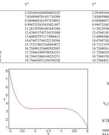
⎦Table 1: Value functions for exponential claims with λ = 2, α = 0.5, p = 6, δ = 0.1, h = -1.0
Y VN VA
A N
6 A
V V
E 100 10
V
−
= × ×
0 5.2916916284504482225 5.2916916569775340804 0.53909198999311822475
1 7.0349589701451734209 7.0349590080700739323 0.53909198998735995256
2 8.5898805261957479052 8.5898805725031060226 0.53909199000546704843
3 9.9947323935433021897 9.9947324474241042348 0.53909198999105221412
4 11.281297001601843380 11.281297062418411890 0.53909198714923774275
5 12.476013745734151800 12.476013812991324764 0.53909184433544653282
6 13.600927971173006613 13.600928044494065528 0.53908864656248120970
7 14.674473744322128506 14.674473823424548999 0.53904774675280347316
8 15.712119625168454872 15.712119709809724483 0.53870051383426619264
9 16.726901524402952093 16.726901614150049118 0.53654346211421986587
10 17.729862499798583231 17.729862593068722008 0.52606238930166806038
11 18.730415860168232371 18.730415950876770156 0.48428469513382021996
12 19.736645071356350220 19.736645139010132209 0.34278258291871530493
Fig. 1: The h-curve for y(10) for 8 iterations using exponential claims H(y) = 1
m m 1
m 1 m 1
t
( t s) m 1
0
L[h (y) h (y)] hH(y)
( )
h ' (y) h
p
for m 2
(t) h (s)e ds
p −
− −
−α − −
− =
λ + δ
⎡ + ⎤
⎢ ⎥
⎢ ⎥ ≥
⎢ αλ ⎥
−
⎢ ⎥
⎢ ⎥
⎣
∫
⎦m m 0 with h(y) h (y)
∞
= =
∑
On solving the scheme (29) up to the third iterate with L d
dy
= , H(y) = 1 we get:
0
y
1
2 y 2
2 y 2 y 2 2 2
h (y) a
( y e )
h (y) ha
p 1
h (y) ha( 2p e y 2p
2
2hp e y 2hp 2h he y
−α
α
α α
=
λ + α δ − λ = −
α
= − α δ + αλ
− α δ + αλ − λ + α δ
y 2 y
y y 2 y y 2 2
0 1 2
4h 4he y 2h y 2e hp
2p e 2e h 4e h )e / (p )
h(y) h (y) h (y) h (y) ...
α α
α α α −α
+ δλ + δλ α − λ α − λ α − α λ + λ − λ δ α
= + + +
(30)
To find the value function, we use:
b
h(y) V (y)
h '(b)
=
The optimal barrier level b*, we solve the equation h”(b*) = 0.
All calculations were done on a Pentium M computer using Maple 7. It should be noted that MATLAB or Mathematica could as well do the job very well.
The numerical solution for exponential claims are compared to the analytical solution in order to test the effectiveness of HAM.
Figure 1 shows the h-curve for the problem and clearly the range of the auxiliary parameter h is (-2,-1). Let bN be the numerical optimal barrier level and bA be the exact optimal barrier.
For twenty iterations; bN =
10.270110761128871629 and bA =
10.270109848973047166.
Table 1 shows the numerically computed dividend value function:
N N
h(y) V
h '(b )
=
Where:
VA = The analytical solution E = The relative percentage error Pareto claims: For Pareto calims:
k
F(s) 1 with , k 0 and s 0
k s α ⎛ ⎞
= −⎜ ⎟ α > ≥ +
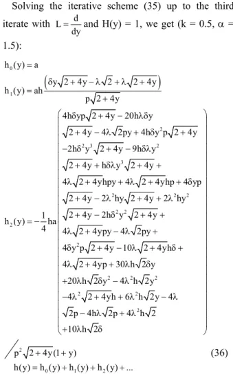
Fig. 2: The h-curve for y(10) for 3 iterations using Pareto claims H(y) = 1
Table 2: Value functions for Pareto claims with λ = 2, k = 0.5, α = 1.5, p = 6, δ = 0.1
y VN
0 21.64588797
2 26.89921874
4 29.61213274
6 31.83177968
8 33.89094615
10 35.89861418
12 37.90169528
14 39.92383481
Then:
y
( 1)
b b b
0
pV ' (y)− λ + δ( )V (y)+ λ
∫
V (y− αs) k (kα +s)− α+ ds=0 (32) And equivalently:y
( 1)
0
ph '(y)− λ + δ( )h(y)+ λ
∫
h(y− αs) k (kα +s)− α+ ds=0 (33) Change of variable results into:y
( 1)
0
ph '(y)− λ + δ( )h(y)+ λ
∫
h(s) k (kα α +(y−s))− α+ ds=0 (34) The iterative scheme (23) thus becomes:0
( 1) 1
0
m 1 m 1
m m 1 ( 1)
m 1 0
m m 0
h (y) a (a is unknown)
( )
L[h (y)] a k (k ( s) ds
p p
( )
h ' ( ) h ( )
p
L[h (y) h (y)] for m 2
k (k ( s))
p h (s)ds
with h(y) h (y)
τ
α − α+
− −
− τ α − α+
− ∞
= =
⎡ λ + δ λ ⎤ = ⎢ − α + τ − ⎥
⎣ ⎦
λ + δ
⎛ τ + τ −⎞
⎜ ⎟
⎜ ⎟
− =⎜ ⎟ ≥
α + τ − λ
⎜ ⎟
⎜ ⎟
⎝ ⎠
=
∫
∫
∑
(35)
Solving the iterative scheme (35) up to the third iterate with L d
dy
= and H(y) = 1, we get (k = 0.5, α = 1.5):
(
)
0
1
2
2 3 2
3
2 2 2
2 2
2
2 h (y) a
y 2 4y 2 2 4y
h (y) ah
p 2 4y 4h yp 2 4y 20h y
2 4y 4 2py 4h y p 2 4y
2h y 2 4y 9h y
2 4y h y 2 4y
4 2 4yhpy 4 2 4yhp 4 yp
2 4y 2 hy 2 4y 2 hy
2 4y 2h y 2 4y
1
h (y) ha
4 4 2 4ypy 4 2py
4 y p 2 4y
=
δ + − λ + λ + =
+
δ + − λδ
+ − λ + δ +
− δ + − δλ + + δλ + + λ + + λ + + δ
+ − λ + + λ
+ − δ + +
= −
λ + − λ +
δ +
2 2 2
2 2
2
2
0 1 2
10 2 4yh
4 2 4yp 30 h 2 y 20 h 2 y 4 h 2y
4 2 4yh 6 h 2y 4
2p 4h 2p 4 h 2
10 h 2
p 2 4y (1 y)
h(y) h (y) h (y) h (y) ...
⎛ ⎞
⎜ ⎟
⎜ ⎟
⎜ ⎟
⎜ ⎟
⎜ ⎟
⎜ ⎟
⎜ ⎟
⎜ ⎟
⎜ ⎟
⎜ ⎟
⎜ ⎟
⎜ ⎟
⎜ ⎟
⎜ ⎟
⎜ − λ + δ + ⎟
⎜ ⎟
⎜ λ + + λ δ ⎟
⎜ ⎟
⎜+ λ δ − λ ⎟
⎜ ⎟
− λ + + λ − λ
⎜ ⎟
⎜ ⎟
− λ + λ
⎜ ⎟
⎜+ λ δ ⎟
⎝ ⎠
+ +
= + + +
(36)
On working further to the more iterations, we notice that on solving for b there is convergence realized both in the numerically computed barrier bN and the value function VN. At the fourth iteration, the barrier approximates to 10.19323790. The value functions are shown in Table 2 and Fig. 2.
DISCUSSION
CONCLUSION
We have derived value functions for both light tailed and heavy tailed distributions representing small and large claims using the HAM. This method can be used to find value functions for the diffusion model. The method gives results that are encouraging and it assures quick convergence to the exact solution. However, it should be noted that this method involves repeated analytical integration and thus only works with symbolic software.
ACKNOWLEDGEMENT
The researchers extend their gratitude to NOMA for the financial support and anonymous referees for the valuable comments.
REFERENCES
Adawi, A., F. Awawdeh and H. Jaradat, 2009. A numerical method for solving Linear Integro Equations. Int. J. Contemp. Math. Sci., 4: 485-496. Avanzi, B., 2009. Strategies for Dividend Distribution:
A review. North Am. Actuarial J., 13: 217-251. Bataineh, A.S., M.S.M. Noorani and I. Hashim, 2008a.
Series solution of the multispecies Lotka-Volterra equations by means of the homotopy analysis method. Differential Equations Nonlinear Mech., 2008: 1-14. DOI: 10.1155/2008/816787
Bataineh, A.S., M.S.M. Noorani and I. Hashim, 2008b. Approximate analytical solutions of systems of PDEs by homotopy analysis method. Comput. Math. Appl., 55: 2913-2923. DOI: 10.1016/j.camwa.2007.11.022
Bataineh, A.S., M.S.M. Noorani and I. Hashim, 2009. Direct solution of nth-order IVPs by homotopy analysis method. Differential Eq. Non Linear Mech., 2009: 1-15. DOI: 10.1155/2009/842094
Buhlmann, H., 1996. Mathematical Methods in Risk Theory. 1st Edn., Springer, USA., ISBN-10: 3540051171, pp: 210.
De Finetti, B., 1957. Su un’ impostazione alternatival della teoria collectiva del rischio. Trans. XVth Int. Cong. Actuaries, 2: 433-443.
El-Nahhas, A., 2007. Analytic Approximations for volterra population Equations. Proc. Pak. Acad. Sci., 44: 255-261.
Gerber, H.U., 1969. Entscheidungskriterien fur den zusammengesetzten Poisson-Prozess. Schweiz. Verein. Versicherungsmath. Mitt., 69: 185-227. Gerber, H.U., 1974. The dilemma between dividends
and safety and a generalisation of the Lundberg-Cramer formulas. Scand. Actuarial J., pp: 46-57. Gerber, H.U., 1979. An Introduction to Mathematical
Risk Theory. 1st Edn., S. S. Huebner Foundation for Insurance Education, Wharton School, University of Pennsylvania, ISBN-10: 0918930081, pp: 164.
Golbabai, A. and M. Javidi, 2007. Application of He’s homotopy perturbation method for nth-order integro-differential equations. Applied Math. Comput., 190: 1409-1416. DOI: 10.1016/j.amc.2007.02.018
He, J.H., 2004. Comparison of homotopy perturbation method and homotopy analysis method. Applied Math. Comput., 156: 527-539. DOI: 10.1016/j.amc.2003.08.008
Jaradat, H., O. Alsayyed and S. Al-Shara, 2008. Numerical solution of linear integro-differential equations. J. Math. Stat., 4: 250-254. DOI: 10.3844/jmssp.2008.250.254
Kasozi, J and J. Paulsen, 2005b. Numerical Ultimate Ruin Probabilities under Interest Force. J. Math. Stat., 1: 246-251. DOI: 10.3844/jmssp.2005.246.251
Kasozi, J. and J. Paulsen, 2005a. Flow of dividends under a constant force of interest. Am. J. Applied Sci., 2: 1389-1394. DOI: 10.3844/ajassp.2005.1389.1394
Liao, S., 2004. Beyond Perturbation: Introduction to the Homotopy Analysis Method. 1st Edn., Chapman
and Hall/CRC, USA., ISBN-10: 158488407X, pp: 322.
Liao, S., 2009. Notes on the homotopy analysis method: Some definitions and theorems. Commun. Nonlinear Sci. Numer. Simul., 14: 983-997. DOI: 10.1016/j.cnsns.2008.04.013
Liao, S.J., 1995. An approximate solution technique not depending on small parameters: A special example. Int. J. Non-Linear Mech., 30: 371-380. DOI: 10.1016/0020-7462(94)00054-E
Lundberg, F., 1903. Approximerad Framst¨allning av Sannolikhetsfunktionen. °Aterf¨ors¨akering av Kollektivrisker. Thesis, Uppsala. http://projecteuclid.org/DPubS?service=UI&versio
n=1.0&verb=Display&handle=euclid.ss/1032280303
Paulsen, J. and H.K. Gjessing, 1997. Optimal choice of dividend barriers for a risk process with stochastic return on investments. Insurance: Math Econ., 20: 215-223. DOI: 10.1016/S0167-6687(97)00011-5 Paulsen, J., 2003. Optimal dividend payouts for
diffusions with solvency constraints. Finance Stoch., 7: 457-473. DOI: 10.1007/s007800200098 Paulsen, J., J. Kasozi and A. Steigen, 2005. A
numerical method to find the probability of ultimate ruin in the classical risk model with stochastic return on investments. Insurance: Math.
Econ., 36: 399-420. DOI: 10.1016/j.insmatheco.2005.02.008
Rawashdeh, E.A., H.M. Jaradat and F. Awawdeh, 2009. Homotopy Analysis Method for delay Integro