Semiparametric Modeling of Daily Ammonia
Levels in Naturally Ventilated Caged-Egg
Facilities
Diana María Gutiérrez-Zapata1,3*, Luis Fernando Galeano-Vasco2,3, Mario Fernando Cerón-Muñoz2,3
1Facultad de Ciencias Exactas y Naturales, Universidad de Antioquia, Medellín, Antioquia, Colombia, 2Facultad de Ciencias Agrarias, Universidad de Antioquia, Medellín, Antioquia, Colombia,3Grupo de Investigación en Genética, Mejoramiento y Modelación Animal (GaMMA), Universidad de Antioquia, Medellín, Antioquia, Colombia
Abstract
Ammonia concentration (AMC) in poultry facilities varies depending on different environ-mental conditions and management; however, this is a relatively unexplored subject in Colombia (South America). The objective of this study was to model daily AMC variations in a naturally ventilated caged-egg facility using generalized additive models. Four sensor nodes were used to record AMC, temperature, relative humidity and wind speed on a daily basis, with 10 minute intervals for 12 weeks. The following variables were included in the model: Heat index, Wind, Hour, Location, Height of the sensor to the ground level, and Period of manure accumulation. All effects included in the model were highly significant (p<0.001). The AMC was higher during the night and early morning when the wind was not
blowing (0.0 m/s) and the heat index was extreme. The average and maximum AMC were 5.94±3.83 and 31.70 ppm, respectively. Temperatures above 25°C and humidity greater
than 80% increased AMC levels. In naturally ventilated caged-egg facilities the daily varia-tions observed in AMC primarily depend on cyclic variavaria-tions of the environmental condivaria-tions and are also affected by litter handling (i.e., removal of the bedding material).
Introduction
Poultry farming in Colombia and other tropical countries depends on naturally ventilated facil-ities where it is difficult to control air quality, resulting in compromised bird welfare and per-formance [1–7]. Ammonia (NH3) formation and emission are inherent to poultry production.
Nitrogenous waste, such as undigested protein and uric acid, in bird excreta are precursors for NH3formation by microbes [8]. Ammonia formation and volatilization is controlled by pH,
temperature (T), moisture and nitrogen (N) content in excreta. Additionally, volatilization depends on factors such as the length of time excreta remains inside the facility, ventilation rates, and the level of gas concentration in the shed [6,8–10]. Therefore, knowing the daily gas fluctuations in response to variations of the above-mentioned conditions is useful to develop in-farm strategies for controlling AMC.
OPEN ACCESS
Citation:Gutiérrez-Zapata DM, Galeano-Vasco LF, Cerón-Muñoz MF (2016) Semiparametric Modeling of Daily Ammonia Levels in Naturally Ventilated Caged-Egg Facilities. PLoS ONE 11(1): e0147135. doi:10.1371/journal.pone.0147135
Editor:Jeffrey Shaman, Columbia University, UNITED STATES
Received:August 9, 2015
Accepted:December 28, 2015
Published:January 26, 2016
Copyright:© 2016 Gutiérrez-Zapata et al. This is an open access article distributed under the terms of the
Creative Commons Attribution License, which permits unrestricted use, distribution, and reproduction in any medium, provided the original author and source are credited.
Data Availability Statement:All relevant data are within the paper and its Supporting Information files.
Generalized additive models (GAM) have been widely used to study the effects of environ-mental components on human health because they are useful to model nonlinear relationships between the response variable and covariates [11–14]. GAM models only differ from general-ized linear models (GLM) in that the linear predictor is replaced by a sum of unknown non-parametric smooth functions of some or all model covariates, allowing a flexible dependence expression of the response variable in the covariates [15–17]. The expression“semi-parametric model”is used when, in addition to nonparametric components (smooth functions), paramet-ric effects (unsmoothed terms) are added to the GAM model [18].
Generalized additive models allow characterizing daily changes of air pollutants without making assumptions about the functional form of the data [11,19]. Furthermore, its additive structure allows to include variables separately, thus increasing the explanatory power of the results [18,20,21]. These models have also been used for studying trends of pollutants associ-ated with vehicle traffic [22–26] and NH3concentration in water and air [27,28], showing
great explanatory power (about 80% of the variation was explained) and adjustment for non-linear relationships between weather variables and gaseous compounds. Furthermore, the model results also highlighted the importance of each effect on the response measured, show-ing trends in temporal and spatial variation of pollutants, thereby allowshow-ing to make inferences.
The aim of this study was to apply GAMs for modeling the curve of daily AMC in a natu-rally ventilated facility for caged layers.
Materials and Methods
This study was approved by the Ethics Committee for Animal Experimentation of Universidad de Antioquia (approved on June 13, 2012).
The farm is owned by the Universidad de Antioquia and it is located in San Pedro de los Milagros (6°26’54.8”N, 75°32’35.2”W), Antioquia province (Colombia, South America). Its use in this study was approved by the Haciendas Department of the Facultad de Ciencias Agrarias. The study was conducted in a naturally ventilated shed occupied with 14406 Loh-mann Brown layers between 42 and 53 weeks of age. The shed included a total of 11 modules. Three of them contained battery cages disposed in three levels (cage measurements: 58 x 34 x 23 cm; length x width x height, respectively) with 6 birds/cage (329 cm2per bird). The remain-ing eight modules had two levels of batteries (cage measurements: 39 x 34 x 23 cm, length x width x height, respectively) with 3 birds/cage (442 cm2per bird).
Two people managed the facility. The feed was produced at the farm and the daily ration was offered manually to the birds during the morning. Water was offeredad libitumthrough drinking cups and nipples. Eggs were collected two times per day. Manure accumulated in piles under the cages, and wood shavings were periodically added to manure in order to control humidity. Sick animals were separated and mortalities were collected daily.
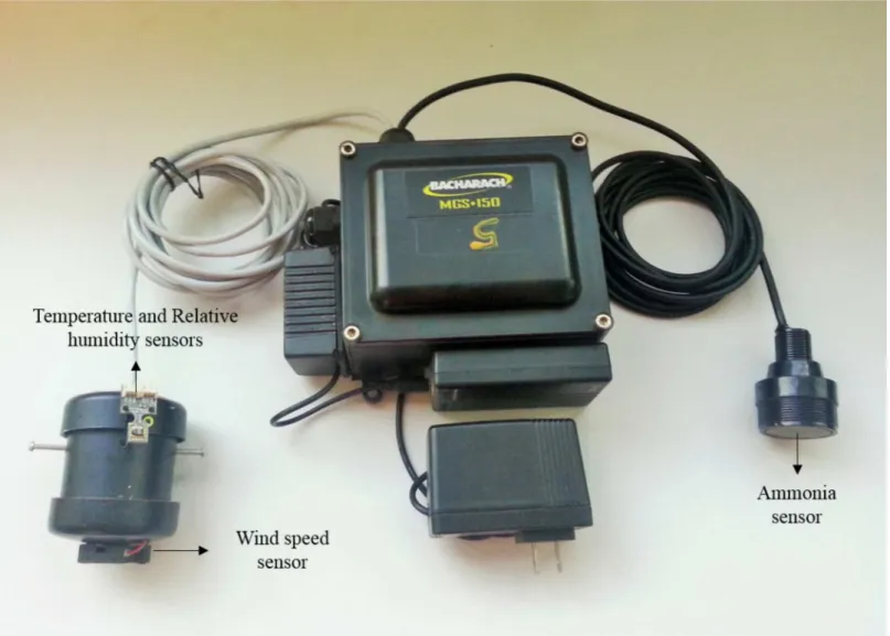
Data were recorded using a multivariable monitoring system composed of four sensor nodes (Fig 1) that simultaneously measured AMC (ppm), T (°C), relative humidity (RH, %), and wind speed (WS, m/s). Sensor node specifications are inS1 Table.
The shed area was divided into 72 parts (4 m wide by 5 m long, each). Within each of these parts we were able to measure at one of four possible heights (heights of the sensor to the ground level were 1.63, 2.12, 2.78, and 3.15 m), so there were 288 possible measuring locations in total. The selection of each location was made at random; once defined, records were taken day and night at 10-minute intervals during one week.
During the 12-week period, 9708 observations from 37 days were considered in the analysis (data inS1 Dataset). Part of the information was lost due to problems with the electrical sys-tem, and some more was discarded for the analysis. Availability of information of at least two Competing Interests:The authors have declared
different sensors and at least 30 records/sensor per day of manure accumulation at each height was set as a requirement for the data debugging process.
The days of manure accumulation in the shed were not consecutive due to loss of informa-tion. Therefore, considering the time spacing and AMC mean values, the days of manure accu-mulation were grouped into eight periods. Periods of manure accuaccu-mulation (PMA) were defined as follows: PMA 1 corresponds to the first 3 days of storage; PMA 2 days 4 to 6; PMA 3 days 7 to 9; PMA 4 days 23 to 25; PMA 5 days 26 to 29; PMA 6 days 29 and 30; PMA 7 days 59 and 60; and PMA 8 days 62, 64, and 65.
The combined effect of T and RH was included in the model as the heat index (HI) pro-posed by Schoen [29]:
HI¼T 1:0799e0:03755T
½1 e0:0801ðD 14Þ
whereTis temperature (°C) andDis the dew point:
237:3g
17:27 g
Fig 1. Measuring equipment (sensor node) used during the study.
where:
g¼
17:27T
237:3þTþln RH= 100
ð Þ
RH: percentage of relative humidity. The GAM model used was:
logðEðY
jklmnpÞÞ ¼aþGjþWkþHlþZmþteðtn;ipÞ þjklmnp
where:
Yjklmnp= Ammonia concentration~ Poi(μ) α= Intercept
Gj= Fixed effect of PMA, wherejranges from 1 to 8 periods.
Wk= Fixed effect of wind, wherekrefers to absence (WS = 0.0 m/s) or presence (WS>0.0 m/s) of wind.
Hl= Fixed effect of height of the sensor to the ground level, wherelvaries from 1 to 4 heights.
Zm= Fixed effect of the location, withm = 1,2,. . .,15locations.
te(tn,ip)= Smooth function of then-th hour of the day andp-th heat index.
jklmnp= Residual effect.
The scale parameter of the Poisson distribution was included as unknown in the model in order to model over dispersion. Hour and Location were variables added in order to account for the effects of time and space. A cyclic cubic regression spline was used for Hour to ensure consistency between initial and final points. The Gam procedure of mgcv library of R program was used for the analysis [30]. Adjusted R2and Generalized Cross Validation (GCV) were used for model selection, with the best fit corresponding to the highest R2and lowest GCV.
Results and Discussion
Both GAM and generalized linear models allow for non-constant variance structures, and errors should be approximately independent [18,31,32]. The residual plot (graphic not included) showed no patterns of residual distribution as they were randomly distributed around zero. Autocorrelation tests were conducted until the fifth lag, finding low correlations (maximum 0.29 in the fourth lag), indicating the absence of autocorrelation between residuals. All variables included in the model had an effect on it (p<0.001).
The adjusted R2of the model was 41.50%, which is between 27 and 70% reported elsewhere [33,34]. Richards et al. [27] used GAM to model AMC in estuary water in Australia. Their R2 was 88.10%. The high fit of their model could be due to the analysis of AMC in an environment different from that of the present study. According to Seedorf and Hartung [35] it is necessary to analyze many variables to determine all process interactions to account for differences in AMC inside animal facilities.
The maximum AMC was 31.70 ppm and the adjusted mean concentration was 5.94 ±3.83 ppm, these values are within those reported in the literature for layersTable 1. Groot et al. [36] reported mean concentrations varying between 8 and 27.10 ppm in broilers. Alloui et al. [1] reported 16.50 and 31.50 ppm AMC for naturally ventilated broiler facilities in sum-mer during the third and seventh weeks of age respectively, while AMC did not exceed 20 ppm in forced-ventilation systems. The differences found in all these studies can be attributed, among others, to changes in ventilation rates through the season, the ventilation system used, and differences in manure management.
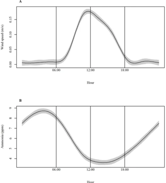
high speeds can also dilute NH3and promote manure drying, limiting NH3formation [8,36, 45,46]. The average AMC was high from 22:00 until the early morning, and low around noon Table 1. Ammonia concentration in laying hen facilities located in different countries and production systems.
Country/year Type of facility/ Ventilation
Manure handling Season Temperature (°C)
Relative humidity (%)
AMC (ppm)
England (1998) [36] BC S; W 10.1a 11.9a(29%)b
The Netherlands (1998) [36] BC S; W 9.8a 5.9a(30%)b
Denmark (1998) [36] BC S; W 8.4a 6.1a(39%)b
Germany (1998) [36] BC S; W 10.5a 1.6a(27%)b
USA (Iowa, 2003) [37] CC; MV HR (BF) 47a
USA (Iowa, 2003) [37] MV MB (D) 2.7a
USA (Iowa, 2003) [38] CC; MV HR (BF) 9.4±11.4c,d 71.0±12.9c,d 44.8
(70.4%)b USA (Pennsylvania, 2003–2004)
[38]
CC; MV HR (BF) 11.1±10.3c,d 77.1±9.2c,d 35.9
(56.4%)b
USA (Iowa, 2003) [38] CC; MV MB (D) 9.4±11.4c,d 71.0±12.9c,d 2.80
(60.4%)b USA (Pennsylvania, 2003–2004)
[38]
CC; MV MB (TW) 11.1±10.3c,d 77.1±9.2c,d 5.2 (65.2%)b
USA (Iowa, 2006) [39] CC; MV HR (BF) W 18.8–22.8e 41
–56e 8
–20e
USA (Iowa, 2006) [39] CC; MV HR (BF) S 28.3–30.1e 46
–53e 2
–4e
USA (Iowa, 2006) [39] CC; MV MB (D) W 22.6–27.1e 36
–47e 6
–8e
USA (Iowa, 2006) [39] CC; MV MB (D) S 30–31e 71–73e 2–8e
USA (Iowa, 2006) [39] CC; NV FR (BF) W 11.4–16.8e 62
–69e 20
–59e
USA (Iowa, 2006) [39] CC; NV FR (BF) S 24–25.5e 62
–66e 3
–15e
Norway, 2008 [40] FS; MV FR (BF) 21.4±0.09c 58±2.1c 98.2±14.1c
Norway, 2008 [40] MS; MV (W) 16.1±0.44c 65±2.5c 32.3±6.8c
Norway, 2008 [40] FC; MV (TW) 14.5±2.01c 5.2±4.1c
China (2011) [41] CC; NV (D) SP 3.27±1.42c
China (2011) [41] CC; NV (D) S 3.13±1.85c
China (2011) [41] CC; NV (D) A 7.96±3.55c
China (2011) [41] CC; NV (D) W 9.66±2.27c
China (2011) [41] CC; NV (D) AN 21a(12.9
–31.5)e 69a(25
–95)e 5.97±3.27c
Taiwan (2011) [42] CC; HS FR 4.5±2.5c
USA (Iowa, 2011–2012) [43] AV MB (1/3 D); FR (BF)
23.4±0.3c 64±3c 5.2±0.5c
USA (Midwest, 2011–213) [44] CC; MV MB; (3-4D) 24.6±1.9c 57±9c 4.0±2.4c
USA (Midwest, 2011–213) [44] AV;MV MB (3-4D); FR (BF)
26.7±1.1c 54±7c 6.7±5c
USA (Midwest, 2011–213) [44] EC; MV MB; (3-4D) 25.2±1.3c 56±9c 2.8±1.7c
BC, Battery cages; S, Summer; W, Winter; CC, Conventional cages; MV, Mechanical ventilation; HR, High-rise; (BF), Betweenflocks; MB, Manure belt; (D), Daily; (TW), Twice a week; NV, Natural ventilation; FR, Floor-rise; FS, Floor housing; MS, Multilevel system; (W), Weekly; FC, Furnished cages; SP, Spring; A, Autumn; AN, Annual; HS, Half-sheltered (T control by moisture); AV, Aviary house; (1/3D), One-third of the manure belt length was removed daily; (3-4D), Manure was removed every 3 to 4 days; EC, Enriched colony house.
aMean bCoef
ficient of variation cMean±SD
dDaily means outside the house eRange of variation
and early afternoon. This coincided with the pattern of daily WS variations recorded in the shed, with top speeds from around noon until the evening, as shown inFig 2.
This is similar to findings by Zhu et al. [41] who studied gas concentration and emission in naturally ventilated facilities for layers in China. They reported that gas concentration was directly influenced by environmental conditions with the highest values observed at night, when temperature and ventilation rates were lower. Different studies have shown the existence of patterns in NH3concentration and emission to the atmosphere depending on season and
hour of the day [41,47–49]. Harper et al. [45] observed that most NH3emissions occur in the
afternoon and evening, and the lowest at night. In addition, Calvet et al. [33] found higher con-centrations at night and during winter compared to summertime. They attributed it to changes in ventilation rates, which were higher in the warmest hours of the day and during the summer. They also found that NH3concentration and emission was negligible in the first days of the
flock, increasing progressively with bird size and feed intake. Fig 2. Daily variations of wind speed (A) and ammonia concentration (B).
Ventilation rate of naturally ventilated facilities is affected by factors such as the number of animals in the shed, and also by the design, orientation and equipment in the facility [50–52]. Birds form living barriers that influence wind distribution within the system, changing the air flow and affecting ventilation in some areas. This affects factors such as T, RH and gasses con-centration. The present study only recorded WS in the sampling locations at the time of mea-surement; accordingly, the dynamics of this flow is not known, so it is not possible to be precise about the extent of its effect in this study.
Both T and RH affect microbial activity so they are directly involved in NH3formation and
emission [53,54]. The highest mean T was observed between 10:00 and 15:00 (fluctuating from 21 to 23°C) while the mean RH ranged from 61 to 67%. The opposite occurred during the cool hours; in the evening or early morning the mean T fluctuated between 14 and 16°C, with 83 to 85% RH.
The AMC fluctuations in time presented a sinusoidal pattern (in the form of sine and cosine functions) similar to that observed by Calvet et al. [33] and Estellés et al. [55] who modeled NH3
concentration and emission. In the present study, the day started with high AMC, then decreased from around 10:00 until 18:00, and increased again at night after 22:00. The AMC daily variation is attributed to diurnal cycles of T and ventilation, which also showed sinusoidal patterns.
High T generates increased NH3formation and volatilization because of increased microbial
degradation of uric acid and proteins. Meanwhile, ventilation helps to release NH3from the
manure into the environment [36].The AMC was lower in the hottest hours, probably due to the increased ventilation during those periods (Fig 2). According to several researchers, high air-exchange rates can limit AMC in a facility as a result of the acceleration of NH3output (higher
emissions), its dilution in the air, and because it promotes manure drying [33,36,41,45,49]. Wind speed was lower and RH increased during the night and early morning. The RH pro-motes increased manure moisture, which is positively related to NH3production due to
increased microbial degradation of uric acid. High RH values can reduce the rate of manure drying. Increasing RH from 45 to 75% generates higher AMC, while decreasing manure mois-ture reduces NH3formation because the amount of NH3-N contained therein is lower [10,33, 35,46,56–59].
A significant correlation between T and RH was observed (-0.69;p<0.05), so the HI pro-posed by Schoen [29] was used in order to include both effects in the model. The HI values were higher than 30°C for extreme T (>30°C), and lower than 15°C for extreme RH (>80%).
Ammonia levels remained low during the day when HI was less than 15°C (Fig 3). The AMC increased from around noon until 18:00, when HI was higher than 30°C; however, the largest AMC were observed in the morning and evening hours (ends of the figure), when HI was between 15 and 20°C.
Accordingly, optimal conditions for low NH3levels are close to the thermo neutral zone
(between 13 and 24°C and 50 to 70% RH) [60,61] of the birds for most of the day (06:00–18:00 hours). In this range, the lowest concentrations were observed when HI was close to 25, corre-sponding to T between 20 and 24°C and RH between 50 and 60%. This indicates that maintain-ing a suitable environment within the facility helps prevent heat stress in the birds and
contributes to improved air quality due to greater control over the formation and release of harmful gases such as NH3. The pattern observed inFig 3is consistent with the cyclical
varia-tions recorded daily inside the shed.
the air, which promotes drying and therefore reduces NH3volatilization. It is important to take
into account that usage of wood shavings or other material to counter humidity was low during PMA 2. Moreover, air flow into the facility has an unknown pattern, so there can be areas where the air does not flow or it is insufficient.
Removal of poultry manure from the shed should also be considered. Manure removal begins around the second month of storage. Since the removal process helps release NH3the
values found during this period are highly variable, regardless of the accumulation period asso-ciated with the location. As the manure removal process can take several days, some areas have few days of manure accumulation (where manure has been already removed), while other areas continue accumulating during 60 or more days. In this case air flow is the most important factor to consider as the cause of variation. Manure management consisted of forming piles under the cages and adding wood shavings to control excessive moisture. The length of the manure accumulation periods was determined by labor availability to take the manure piles out of the building, which could last two weeks or more. The maximum accumulation period recorded for an area was 75 days.
Besides the above mentioned factors it is known that NH3levels are directly affected by
other components such as management activities (feeding, cleaning, etc.), animal density and age, and design of the facility, among others [33,36,45,49–52,63].
According to the analysis, when the height of the sensor to the ground level increases from 1.63 to 2.12 m the NH3levels decrease in 0.46 ppm. However, AMC increased 1.29 ppm at 2.78
m and then decreased 0.67 ppm at 3.15 m. According to Tinôco [61], there are three layers of air in a naturally-ventilated poultry facility: an upper layer of hot air and high NH3and H2S
concentrations, a middle layer with newly introduced air, and a lower layer of cool air which is heated on contact with the birds and receives the CO2they generate. After being released from
manure, NH3is carried horizontally by the wind while it is dispersed in a lateral and vertical
movement [54]. As NH3is lighter than air, it is possible for it to quickly move to the top of the
facility and therefore it should be detected in higher concentrations there. However, the pattern observed in the present study varied between heights, and only a minor difference between concentrations was observed at more than 2.12 m. According to some studies, air flow is Fig 3. Ammonia concentration as a smooth function of hour and heat index.Ammonia level is higher in the yellow areas compared to the red ones.
continuous above 2 m because fewer elements are located at that height, thus air flow is not interrupted; additionally, wind speed is lower, so gas concentration tends to be constant at the top and less predictable at the bottom [64,65]. To adequately characterize AMC variations with regard to height, it is necessary to establish the airflow dynamics within the facility, which is difficult in open sheds because of the number and complexity of the intervening variables (e.g. turbulent transport).
Even though the mean NH3levels observed in this study were less than 10 ppm, at times
NH3values were close to the safe exposure limits for humans during an 8-hour period set by
US agencies between 25 and 50 ppm [66,67]. In poultry production there is no legal limit for exposure of birds to NH3; however, levels below 10 ppm are generally considered adequate for
proper animal welfare and performance, with a maximum of 25 ppm at the height of the bird [68,69]. The maximum exposure to NH3levels greater than or equal to 25 ppm was 310
min-utes (5 hours; between 01:00 and 06:00). Negative effects of NH3on birds or staff have been
widely reported [1,3,5,7,66,70–77]. Since the effects depend on both gas concentration and time of exposure it would be necessary to further investigate whether exposure to low AMC has cumulative effects in hens during a full production cycle.
Conclusions
Daily AMC variations depend on cyclical changes of environmental conditions (T, RH and WS). Temperature and humidity above 25°C and 80% favor increased NH3levels in naturally
ventilated facilities.
Generalized additive models are a suitable alternative for analyzing nonlinear relationships, such as daily NH3variations and environmental factors. However, it is essential for a good fit
to include the greatest possible number of factors affecting NH3, especially those related to the
source of the gas (N, T, humidity, and pH of manure) and those associated with its release (air T and turbulent transport).
Supporting Information
S1 Dataset. This file contains the database used for the analysis presented in this work.
Information of each column corresponds to: Zone of measurement (zone), date, hour, RH (humidity), T (temperature), AMC (ammonia), wind speed (windspeed), nodo, days of manure acummulation (dma), Height (height), Hour (hourofday (s)), WS (ws), PMA (pma) and HI (hi). (CSV)
S1 Table. Specifications of the monitoring system.
(DOCX)
Acknowledgments
The authors acknowledge the support of the Comité para el Desarrollo de la Investigación CODI of Universidad de Antioquia through the E01533 "Design and validation of decision support systems for commercial-egg poultry farms" and the Estrategia de Sostenibilidad (Sus-tainability Strategy) CODI-UdeA 2016 projects granted to GaMMA research group.
Author Contributions
References
1. Alloui N, Alloui MN, Bennoune O, Bouhentala S. Effect of ventilation and atmospheric ammonia on the health and performance of broiler chickens in summer. J World's Poult Res. 2013; 3(2):54–6. 2. National Research Council (NRC). Air emissions from animal feeding operations: Current knowledge,
future needs. Final report. United States: The National Academies Press; 2003. p. 225.
3. Deaton JW, Reece FN, Lott BD. Effect of atmospheric ammonia on laying hen performance. Poult Sci. 1982; 61(9):1815–7. PMID:7134135
4. Fidanci UR, Yavuz H, Kum C, Kiral F, Ozdemir M, Sekkin S, et al. Effects of ammonia and nitrite-nitrate concentrations on thyroid hormones and variables parameters of broilers in poorly ventilated poultry houses. J Anim Vet Adv. 2010; 9(2):346–53.
5. Miles DM, Branton SL, Lott BD. Atmospheric ammonia is detrimental to the performance of modern commercial broilers. Poult Sci. 2004; 83(10):1650–4. PMID:15510548
6. Ritz CW, Fairchild BD, Lacy MP. Implications of ammonia production and emissions from commercial poultry facilities: A Review. J Appl Poult Res. 2004; 13(4):684–92.
7. Wang YM, Meng QP, Guo YM, Wang YZ, Wang Z, Yao ZL, et al. Effect of atmospheric ammonia on growth performance and inmmunological response of broiler chickens. J Anim Vet Adv. 2010; 9 (22):2802–6.
8. Atapattu NSBM, Serenata D, Belpagodagamage UD. Comparison of ammonia emission rates from three types of broiler litters. Poult Sci. 2008; 87(12):2436–40. doi:10.3382/ps.2007-00320PMID: 19038797
9. United States Environmental Protection Agency (EPA). National emission inventory-ammonia emis-sions from animal husbandry operations. Draftreport. United States2004. p. 131.
10. Patterson PH, Adrizal. Management strategies to reduce air emissions: Emphasis-dust and ammonia. J Appl Poult Res. 2005; 14(3):638–50.
11. Dominici F, McDermott A, Zeger SL, Samet JM. On the use of generalizedadditive models in time-series studies of air pollution and health. Am J Epidemiol. 2002; 156(3):193–203. PMID:12142253 12. Fairley D. Daily mortality and air pollution in Santa Clara County, California: 1989–1996. Environ Health
Perspect. 1999; 107(8):637–41. PMID:10417361
13. Schwartz J, Dockery DW, Neas LM. Is daily mortality associated specifically with fine particles? J Air Waste Manag Assoc. 1996; 46(10):927–39. PMID:8875828
14. Terzi Y, Cengiz MA. Using of generalized additive model for model selection in multiple poisson regres-sion for air pollution data. Sci Res Essays. 2009; 4(9):867–71.
15. Clark M. Generalized Additive Models. Getting started with additive models in R. Center for Social Research, University of Notre Dame; 2013.
16. Díaz Z, Fernández J, Heras A, Pozo ED, Vilar JL. Modelos aditivos generalizados aplicados al análisis de la probabilidad de siniestro en el seguro del automóvil. Madrid: Universidad Complutense de Madrid. Facultad de Ciencias Económicas y Empresariales. Campus de Somosaguas; 2013. 17. Tobías A, Saez M. Time-series regression models to study the short-term effects of environmental
fac-tors on health. Departament d’Economia, Universitat de Girona 2004.
18. Wood SN. Generalized Additive Models: an introduction with R: Taylor & Francis; 2006. 384 p. 19. Ramsay TO, Burnett RT, Krewski D. The effect of concurvity in generalized additive models linking
mor-tality to ambient particulate matter. Epidemiology. 2003; 14(1):18–23. PMID:12500041 20. Hastie T, Tibshirani R. Generalized Additive Models. Statist Sci. 1986; 1(3):297–310. 21. Hastie TJ, Tibshirani RJ. Generalized Additive Models: Taylor & Francis; 1990.
22. Aldrin M, Hobæk I. Generalised additive modelling of air pollution, traffic volume and meteorology. Atmos Environ. 2005; 39(11):2145–55.
23. Carslaw DC, Beevers SD, Tate JE. Modelling and assessing trends in traffic-related emissions using a generalised additive modelling approach. Atmos Environ. 2007; 41(26):5289–99.
24. Li L, Wu J, Hudda N, Sioutas C, Fruin SA, Delfino RJ. Modeling the concentrations of on-road air pollut-ants in Southern California. Environ Sci Technol. 2013; 47(16):9291–9. doi:10.1021/es401281rPMID: 23859442
25. Reina J, Olaya J. Ajuste de curvas mediante métodos no paramétricos para estudiar el comporta-miento de contaminación del aire por material particulado PM10. Rev EIA Esc Ing Antioq. 2012; 18:19– 31.
27. Richards R, Chaloupka M, Strauss D, Tomlinson R. Using generalized additive modelling to understand the drivers of long-term nutrient dynamics in the broadwater estuary (a subtropical estuary), Gold Coast, Australia. Journal of Coastal Research. 2014; 30(6):1321–9.
28. Staelens J, Wuyts K, Adriaenssens S, Avermaet PV, Buysse H, Bril BVd, et al. Trends in atmospheric nitrogen and sulphur deposition in northern Belgium. Atmos Environ. 2012; 49:186–96
29. Schoen C. Empirical model of the emperature–humidity index. J Appl Meteor. 2005; 44(9):1413–20. 30. R Core Team. R: A language and environment for statistical computing. Vienna, Austria R Foundation
for Statistical Computing; 2013.
31. Guisan A, Edwards TC Jr, Hastie T. Generalized linear and generalized additive models in studies of species distributions: Setting the scene. Ecol Modell. 2002; 157(2–3):89–100.
32. Venables WN, Dichmont CM. GLMs, GAMs and GLMMs: An overview of theory for applications in fish-eries research. Fish Res. 2004; 70(2–3):319–37.
33. Calvet S, Cambra M, Estellés F, Torres AG. Characterization of gas emissions from a Mediterranean broiler farm. Poult Sci. 2011; 90(3):534–42. doi:10.3382/ps.2010-01037PMID:21325223
34. Rumburg BP. Differential optical absorption spectroscopy (doas) measurements of atmospheric ammo-nia in the mid-ultraviolet from a dairy. Washington: Universidad Estatal de Washington; 2006. 35. Seedorf J, Hartung J. Survey of ammonia concentrations in livestock buildings. J Agric Sci. 1999; 133
(4):433–7.
36. Groot PWG, Metz JHM, Uenk GH, Phillips VR, Holden MR, Sneath RW, et al. Concentrations and emis-sions of ammonia in livestock buildings in Northern Europe. J agric Engng Res. 1998; 70(1):79–95. 37. Xin H, Liang Y, Gates RS, Wheeler EF, editors. Ammonia emission from Iowa layer houses.
Proceed-ings of the Midwest Poultry Federation Convention; 2004; St. Paul, MN.
38. Liang Y, Xin H, Wheeler EF, Gates RS, Li H. Ammonia emission for US poultry houses: Laying hens. 2004 ASAE/CSAE Annual International Meeting; 1–4 August; Ottawa, Ontario, Canada 2004. 39. Green AR, Wesley IV, Trampel DW, Xin H. Air quality and bird health status in three types of
commer-cial egg layer houses. J Appl Poult Res. 2009; 18(3):605–21.
40. Nimmermark S, Lund V, Gustafsson G, Eduard W. Ammonia, dust and bacteria in welfare-oriented sys-tems for laying hens. Ann Agric Environ Med. 2009; 16(1):103–13. PMID:19630203
41. Zhu Z, Dong H, Zhou Z, Xin H, Chen Y. Ammonia and greenhouse gases concentrations and emissions of a naturally ventilated laying hen house in Northeast China. Trans ASABE. 2011; 54(3):1085–91. 42. Cheng W-H, Chou M-S, Tung S-C. Gaseous ammonia emission from poultry facilities in Taiwan.
Envi-ron Eng Sci. 2011; 28(4):283–9.
43. Zhao Y, Xin H, Shepherd TA, Hayes MD, Stinn JP, Li H. Thermal environment, ammonia concentra-tions, and ammonia emissions of aviary houses with white laying hens. Trans ASABE. 2013; 56 (3):1145–56.
44. Zhao Y, Shepherd TA, Li H, Xin H. Environmental assessment of three egg production systems–part I: Monitoring system and indoor air quality. Poult Sci. 2015; 94(3):518–33. doi:10.3382/ps/peu076PMID: 25737567
45. Harper LA, Flesch TK, Wilson JD. Ammonia emissions from broiler production in the San Joaquin Val-ley. Poult Sci. 2010; 89(9):1802–14. doi:10.3382/ps.2010-00718PMID:20709964
46. Miles DM, Rowe DE, Cathcart TC. Litter ammonia generation: Moisture content and organic versus inorganic bedding materials1. Poult Sci. 2011; 90(6):1162–9. doi:10.3382/ps.2010-01113PMID: 21597054
47. Fiedler AM, Müller H-J. Emissions of ammonia and methane from a livestock building natural cross ven-tilation. Meteorologische Zeitschrift. 2011; 20(1):59–65.
48. O’Shaughnessy PT, Achutan C, Karsten AW. Temporal variation of indoor air quality in an enclosed swine confinement building. J Agric Saf Health. 2002; 8(4):349–64. PMID:12549241
49. Zhang G, Strøm JS, Li B, Rom HB, Morsing S, Dahl P, et al. Emission of ammonia and other contami-nant gases from naturally ventilated dairy cattle buildings. Biosystems Engineering. 2005; 92(3):355– 64.
50. Food and Agriculture Organization of the United Nations (FAO). Rural structures in the tropics. Design and development. Rome2011.
51. Green AR, Xin H. Effects of stocking density and group size on heat and moisture production of laying hens under thermoneutral and heat‐challenging conditions. Transactions of the ASABE. 2009; 52 (6):2027–32.
53. Gyldenkærne S, Ambelas C, Hertel O, Ellermann T. A dynamical ammonia emission parameterization for use in air pollution models. J Geophys Res Atmos. 2005; 110(D7):1–14.
54. Harper LA. Ammonia: Measurement issues. Lincoln, Nebraska: USDA Agricultural Research Service; 2005.
55. Estellés F, Calvet S, Ogink NWM. Effects of diurnal emission patterns and sampling frequency on preci-sion of measurement methods for daily ammonia emispreci-sions from animal houses. Biosystems Engineer-ing. 2010; 107(1):16–24.
56. Carey JB, Lacey RE, Mukhtar S. A Review of literature concerning odors, ammonia, and dust from broiler production facilities: 2. Flock and house management factors. J Appl Poult Res. 2004; 13 (3):509–13.
57. Singh A, Casey KD, King WD, Pescatore AJ, Gates RS, Ford MJ. Efficacy of urease inhibitor to reduce ammonia emission from poultry houses1. J Appl Poult Res. 2009; 18(1):34
–42.
58. Yang P, Lorimor JC, Xin H. Nitrogen losses from laying hen manure in commercial high-rise layer facili-ties. Trans ASAE. 2000; 43(6):1771–80.
59. Yang P, Loromor JC, Powers WJ, Zhang R. Retaining nitrogen in layer manure by restraining ammonia emission. ASAE Annual Meeting: American Society of Agricultural and Biological Engineers; 2002. 60. Kilic I, Simsek E. The effects of heat stress on egg production and quality of laying hens. J Anim Vet
Adv. 2013; 12(1):42–7.
61. Tinôco IFF. Avicultura Industrial: Novos conceitos de materiais, concepções e técnicas construtivas disponíveis para galpões avícolas brasileiros. Rev Bras Cienc Avic. 2001; 3(1).
62. Neijat M, House JD, Guenter W, Kebreab E. Production performance and nitrogen flow of Shaver White layers housed in enriched or conventional cage systems. Poult Sci. 2011; 90(3):543–54. doi:10. 3382/ps.2010-01069PMID:21325224
63. Xin H, Gates RS, Green AR, Mitloehner FM, Jr PAM, Wathes CM. Environmental impacts and sustain-ability of egg production systems1. Emerging issues: Social Sustainability of Egg Production Sympo-sium: Poult Sci. 2011. p. 1–15.
64. Fiedler M, Saha CK, Ammon C, Berg W, Loebsin C, Sanftleben P, et al. Spatial distribution of air flow and CO2concentration in a naturally ventilated dairy building. Environ Eng Manage J. 2014; 13 (9):2193–200.
65. Mendes LB, Edouard N, Ogink NWM, Dooren HJCv, Tinôco IdF, Mosquera J. Spatial variability of mix-ing ratios of ammonia and tracer gases in a naturally ventilated dairy cow barn. Biosystems Engineer-ing. 2015; 129:360–9.
66. U.S. Department of Health and Human Services (DHHS). Toxicological profile for ammonia. In: Public Health Service, Agency for Toxic Substances and Disease Registry (ATSDR), editor. 2004.
67. U.S. Department of Health and Human Services (DHHS), U.S. Department of Labor. Occupational safety and health guideline for ammonia. 1992:1–7.
68. The National Chicken Council (NCC). National Chicken Council animal welfare guidelines and audit checklist for broilers. 2014.
69. United Egg Producers (UEP). Animal husbandry guidelines for U.S. egg laying flocks. 2010. 70. Alencar M do CB, Nääs I de A, Gontijo LA. Respiratory risks in broiler production workers. Rev Bras
Cienc Avic. 2004; 6(1):23–9.
71. Al-Mashhadani EH, Beck MM. Effect of atmospheric ammonia on the surface ultrastructure of the lung and trachea of broiler chicks. Poult Sci. 1985; 64(11):2056–61. PMID:4070137
72. Anderson DP, Beard CW, Hanson RP. Adverse effects of ammonia on chickens including resistance to infection with Newcastle disease virus. Avian Diseases. 1964; 8(3):369–79.
73. Beker A, Vanhooser SL, Swartzlander JH, Teeter RG. Atmospheric ammonia concentration effects on broiler growth and performance1. J Appl Poult Res. 2004; 13(1):5
–9.
74. Heederik D, Sigsgaard T, Thorne PT, Kline JN, Avery R, Bønløkke JH, et al. Health effects of airborne exposures from concentrated animal eeeding operations. Environ Health Perspect. 2007; 115(2):298– 302. PMID:17384782
75. Donham KJ, Cumro D, Reynolds S. Synergistic effects of dust and ammonia on the occupational health effects of poultry production workers. J Agromedicine. 2002; 8(2):57–76. PMID:12853272
76. Yahav S. Ammonia affects performance and thermoregulation of male broiler chickens1. Anim Res. 2004; 53:289–93.