AUTOMATIC REGULATION AND OPTIMAL CONTROL REGARDING FLUVIAL OR SPATIAL NAVES EQUILIBRIUM STABILIZATION

(1)

“Mircea cel Batran” Naval Academy Scientific Bulletin, Volume XIX – 2016 – Issue 2

The journal is indexed in: PROQUEST / DOAJ / Crossref / EBSCOhost / INDEX COPERNICUS / DRJI / OAJI / JOURNAL INDEX / I2OR / SCIENCE LIBRARY INDEX / Google Scholar / Academic Keys/ ROAD Open Access /

Academic Resources / Scientific Indexing Services / SCIPIO / JIFACTOR

AUTOMATIC REGULATION AND OPTIMAL CONTROL REGARDING FLUVIAL OR

SPATIAL NAVES EQUILIBRIUM STABILIZATION

Mircea LUPU1 Gheorghe RADU2

Cristian-George CONSTANTINESCU3 1

Prof., PhD, “Transilvania” University of Brasov, member of Romanian Scientists Academy 2

Assist. Prof., PhD, “Henri Coanda” Air Force Academy, Brasov 3

Assist. Prof. eng., PhD, “Henri Coanda” Air Force Academy, Brasov

Dedicated to math. Gheorghe Radu, PhD, on his 65-th anniversary

Abstract: The first part of the paper deals with cruise, cargo or underwater naves equilibrium stabilization in case of rolling perturbations. The stabilization conditions are determined by using a hydro-pneumatic automate regulator. Oscillations damping is achieved with a hydro-pneumatic compensator, by using the water tanks that the naves are equipped with.

The second part of the paper deals with automatic stabilization of rockets, submarines or satellites dynamics. This stabilization is based on relay-type automatic regulators, by using the minimal time criterion for optimal control with the Pontreagiune extremal principle. In this study, the state variables are the rotation angles and the control function has 2 components, which are appearing because of lateral rolling perturbations. Finaly, numeric-analytical l studies are approached, and the results are graphically presented.

Key words: optimal control, control function, extreme principle of Pontreaguine, absolute stability.

MSC2010: 34H05, 49K35, 93C15, 93C73, 93D10.

1. INTRODUCTION

The goal of an optimal control problem (O.C.P.) of a dynamic system is to determine a set of state variables, of certain control and driving functions satisfying an optimization criterion, performing the extremization of aq quality index in this way. This performance index is a functional depending on these elements and time and spatial restrictions.. Practical applications requirements for these functionals are optimal controls of the following type: achievement of minimal time, minimum fuel consumption, energy, to achieve extreme performance [4,10,13]. Dynamical systems from different domains are generally represented generally by nonlinear equations with parameters, while internal or external disturbances occur leading to unstable solutions related to a free balance state. The stabilization of these regimes is done by using automatic controls that actually fast reacts for optimal control and routing [3,5-7, 12,14]. Lurie [8], [4], [13] and Popov [11], [4], [3] methods are known to automatically adjust the absolute stabilization, with applications. This paper, for optimal control of stabilizing angular

velocities of aircraft and missiles, deals with the "Minimum Time Criteria" and the Pontreaguine extremal [9], [1], [7], with results and studies in different applications [5][6][7]. The optimal control function will have 2 components: u

(

u₁,u₂

)

. 2. THE SHIPS STABILIZATION IN ROLLING

CASE

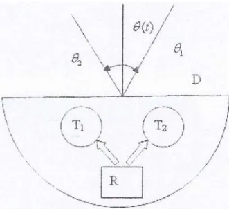
It is known that the maritime or spatial ships are disturbed in their movement (by the waves, wind or other mechanical parameters). The rolling oscillations that they are forced to do are represented in Figure 1 by the rotation angle θ

( )

t , side by a fixed mark. To re-achieve the stable movement regime, these oscillations have to be damped, and this is done by the mashinery presented in Figure 1.

437 DOI: 10.21279/1454-864X-16-I2-066

(2)

Fig. 1: A pump conected to two tanks Basically, it consists in two tanks (T1 and T2)

mounted simetrically of the longitudinal and vertical axis and a system of servo-mechanics and electronical leaded pumps (a hydraulic

regulator, R), which transfer fluid in the tanks, contra-ballancing the rolling oscillations.

The hydraulic regulator is shown in figure 2.

Fig. 2: The hydraulic regulator In this mode of discharge or filling the tanks in

contra ballance with the oscillation amplitude, a spell effect is achieved by the friction and the variation of the fluid mass (left - right), involving the asymptotic stability with intermittences. In the phase space, the spiral trajectories are wavy with the change of the movement sense, tending to the stable asymptotic focus.

The rolling angle θ (Figure 2) is signalized by the rolling indicator 4 in the gyroscopically quadrant

mounted on the ship. So, through the variation of this angle, the server 1 is involved by the pump (ex: in right side) an is opening the input of the fluid in the right half of the servo-motors 2. This produce a displacement r of the bar 3, proprtional with the angle θ.

Simplifying the model, the equation of the system with the free degree θ

( )

t is:

Kr M

Jθ=− θ− (1)

where J is the inertia momentum of the ship, relating the vertical axis which goes through the

438 DOI: 10.21279/1454-864X-16-I2-066

(3)

Academic Resources / Scientific Indexing Services / SCIPIO / JIFACTOR mass centre, θ

( )

t is the rolling angle side by the

0

=

θ , Mθ is the linear momentum of amortization by the friction of the viscous fluid, and r is the displacement of the mechanism arm owing to the rolling. I tis proportional with θ, so that Kr=Nθ. This is considered to be the the reaction momentum, necessary to damp the rolling oscillation, so that the ship returns to its normal course. To accelerate this amortization, the hydraulic absorber must keep the rolling angle in certain limits. In this way, this system is adding an „inverse link” (feedback) 5. The cylinder of the server acquires beside the rolling rotation (to the right) a double pressure. The server valves are closing and its operation is stopped. This is repeated acting to the left side, by discharging the right tank and filling the left one. So, a bigger amortization is achieved because of the momentum Nθ, and after a finite number of oscillations, the ship is stabilized to the null solution by decreasing the rolling oscillation amplitude (amortizing). The link is with „free bearing clearence” and for coulisse 6 an the 2B distance and the server body oscillating in the ±B

space, this mean r±B≈θ, or r=θB, with the „+” sign for θ>0 and the „-” sign for θ<0.

B 2λθ+ω2θ=±ω2

+ θ 

 ₍₂₎

In the phase space, the study of the movement is carried aut in the following way: we are considering the movement right-left with

(

−B,B

)

∈

θ . Denoting θ=x₁+B, (2) becomes:

0 ,

0 x x 2

x₁+ λ₁+ω2 ₁= δ=λ2−ω2<

 (3)

For n2 <k2 we have a low resistance is linearly amortized side by x≡0, having a displacing to the right face of the origin with B. he decrement of the oscillation is ∆=e−nπω. If the displacement is from left to right, then θ=x₂−B, resulting the following equation:

0 x x 2

x₂+ λ₂+ω2 ₂ =

 (4)

The amortization law is the same, but the oscillation will be displaced to the left with B. So, the trajectory in the phase space will trace a logarithmic spiral (figure 3) in the (x, y) plane,

y

x= with the solution for the homogeneous case:

(

C cos t C sin t

)

e

x= −λt ₁ δ + ₂ δ (5)

Fig. 3: The trajectory in the phase space in homogeneous case Then, with θ=x±B for the non-homogeneous

equation, the trajectory presented in figure 4 was obtained graphically: a cut was made on the x’Ox

axis and the upper figure is displaced to the right with B, since the down figure is displaced to the left with B.

439 DOI: 10.21279/1454-864X-16-I2-066

(4)

Fig. 4: The trajectory in the phase space in nonhomogeneous case The spirals are merged by continuity and will

ondulate to origin O thus: considering the initial position at t=0, xi₀ >0, then with recurrence ton the left:

(

−

)

∆− = ∆−

(

+∆

)

=

+ _x _B _B _x _B₁

xi₀1 i₀ i₀ (6)

The point will got o the left side of the origini if:

(

1

)

0

B

xi₀∆− +∆ > or xi₀ B1 1>2B     

∆ + >

(6) is conditioned by 0<xi₀ ≤B.

If B<xi₀≤B

(

1+∆−1

)

, the trajectory falls to origin through the inferior side without cross in the interval (-B , B) – figure 2.

Recalling (1), we obtain (2):

   

↑ θ > θ ω −

↓ θ < θ ω = θ ω + θ λ + θ

; 0 , B

2 ₂

2 2

  

 

The resistance force is a discontinuous pulse (relay type): F

( )

θ =2λθω2θ.

This equation caracterize an intermitent oscillation with a time-decreasing amplitude and the solutions will be recurent, θ_n =θ_n

( )

t , where the initial conditions for θ_n₊₁

( )

t will be

( ) ( )

0 n n 0 n 1

n t =θ t

θ ₊ and t* =t0_n will be the moment

when θ_n

( )

t* =0. We will consider the first phase

( )

t

1

θ =

θ when θ₁

(

t≡0

)

=θ₀ and θ1

( )

0 =0,, B

0 >

θ . The last condition is justified by the particular solutions θ=±B and taking into consideration that for θ₀∈

(

−B,B

)

we have a ballanced regime, see figure 5.

( )

(

δ −ϕ

)

δ ω + =

θ₁ t B a1e−λt cos t

( )

(

δ −ϕ

)

δ ω + − =

θ2n t B a2n e−λt cos t

( )

(

δ −ϕ

)

δ ω + =

θ₂_n₋₁ t B a2n−1e−λt cos t

440 DOI: 10.21279/1454-864X-16-I2-066

(5)

Fig. 5: Rolling amortization

3. OPTIMAL CONTROL IN ANGULAR SPEED STABILIZATION REGARDING FLUVIAL OR SPATIAL NAVES

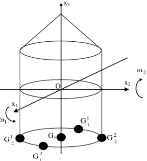
We will consider a multi-engines ship with axial- cylinder symmetry. Figure 6. We choose a system of axes (Ox1x2x3) as principal axes of inertia, where O is the masses, as a solid body rigidly fixed in point O. The vessel rotate with the angular velocity ω

(

ω₁,ω₂,ω₃

)

, where ω_i are the rotation speeds around the axes Oxi, i=1,3; Ox3 is the axis of longitudinal symmetry. Symmetrical with these axes the ship has turbojet propulsion generators G₁

(

G1₁,G₁2

)

on Ox1 with two nozzles,

(

2

)

2 1 2 2 G ,G

G on Ox2 and generator G3 on Ox3,

with traction purpose. These reactive nozzles can create moments, being accompanied by gas dynamics wings, integrating gyroscopes, small jet shutters that can help to guide and stabilize the angular velocities regime. The controller [3], [5-7] is equipped with sensors and microprocessors for data processing and it may (with a rapid response) control the disrupted regime for optimal stabilization [12], [14]. Disturbances considered here may be due to turbines fuel, meteo external agents or environmental density. These naves may be rockets, spacecraft, capsule, modules, megadrones or submarines, torpedoes, etc [8], [12], [14].

Fig. 6: A multi-engine ship

t B

-B

θ

0

θ

δ π =

1 t

δ π =2

t2

x1

1

ω

x2

x3

O

2

ω

1

G

2

1

G 1

2

G G22

G3

441 DOI: 10.21279/1454-864X-16-I2-066

(6)

The angular velocities are ω₁=x₁

( )

t , ω₂ =x₂

( )

t ,

( )

t

x₃ 3 =

ω , the inertia momentums of the body are I1, I2, I3 - simetrically

(

I₁ =I₂ =I

)

, see figura 6.

We write the equations of angular velocities disturbed by external moments M_i

( )

t [10], [12], [14]:

(

)

( )

(

)

( )

(

)

( )

     + − = + − = + − = t M x x I I x I t M x x I I x I t M x x I I x I 3 2 1 2 1 3 3 2 3 1 1 3 2 2 1 3 2 3 2 1 1    (1)

We suppose that moments Mi(t) are caused by propelling forces G

(

g₁,g₂,g₃

)

:

( )

t g l

h₁= ⋅ ₁ , h₂ =l⋅g₂

( )

t , h₃ =l⋅g₃

( )

t (2) And taking into consideration the simetry

I : I

I1 = 2 = , we have:

( )

         = + − − = + − = t g I h x t g I l x x I I I x t g I l x x I I I x 3 3 3 1 1 3 2 2 1 3 2 3 1    (3)

System (1) with Mi

( )

t =0 is in stable equilibrium around O

(

0,0,0

)

(undisturbed).

Let’s suppose that at t0 =0 we have the disturbed position

( )

1 1 0

x =α , x₂

( )

0 =α₂, x₃

( )

0 =α₃ (4) If the traction g3(t) is known, than we have

( )

=α +

_∫

( )

τ τ t

0 3 3 3

3 g d

I h t

x (5)

This shows that x3 can be controlled independently of x1 and x2, but x3 can influence in (3) variables x1 and x2. We suppose that the rapid reaction response time is short and x3 may be considered constant x₃ =α₃, so g₃ ≅0. We also suppose that forces g1, g2 are bounded

( )

t L

g₁ ≤ , g₂

( )

t ≤L (6) In this case the system (3) is linearized and we introduce the control function u

(

u₁

( ) ( )

t ,u₂ t

)

to control optimum stabilization of disturbed solution to O (x1=0, x2=0) for system (7) in minimal time.

( )

   ≡ + ω − = ≡ + ω = 2 2 1 2 1 1 2 1 f t ku x x f t ku x x   (7) where:

( )

        = = > = > ω α − = ω 2 , 1 i ; L t g t u 0 k ; L I l k 0 ; I I I i i 3 3 (7’)

We note that state equations (7) in the phase space

(

x₁Ox₂

)

, X

(

x1

( ) ( )

t ;x2 t

)

, with control parameters

(

u₁

( ) ( )

t ;u₂ t

)

satisfy the conditions:

( )

; U:

[

1,1

]

1 t u 1 1 t u 1 2

1 ₌ ₋

   ≤ ≤ − ≤ ≤ − (8)

and hence the allowable plan U (u1Ou2) is a compact square.

The technical sense in equations (7) for Ui (t) is to find forces g_i

( )

t ↔u_i

( )

t to reduce speeds

(

x₁,x₂

) ( )

→ 0,0 on optimal paths starting from

(

1 2

)

0 ,

M α α at time t0 to reach the final target O (0, 0) at the time tf> t0 so the transfer time to be minimal (o.c.p.) [2], [3], [9], [7].

4. MINIMAL TIME CRITERION. EXTREMUM PRINCIPLE

Let’s consider a system described by the state equations

( ) ( )

(

t,xt ,ut

)

,t

[

t ,t

]

,i 1,n f

x_i = _i ∈ ₀ ₁ ⊆R₊ = (9) where the state function is

( ) (

)

n

i n 2

1,x ,...,x ,x X x

t

x = ∈ ⊂R and the control

function u

( ) (

t = u₁,u₂,...,u_m

)

⊂U⊂Rm with n

m≤ .

Functions fi meet the regularity conditions and U is the allowable domain of parameters ui(t). System (9) respects the given initial conditions (I):

(I)

x

_i

( )

t

₀

=

x

0_i

∈

R

,

i

=

1 ,

n

(10) determining the disturbed initial state X0∈S0, where S0 is the variety on which X0 is fixed. Assuming that Cauchy problem (9) (10) has

(

0 0

)

0

i

i x t,t ,x ,u,t t

x = ≥ as unique solution, we request that this trajectory transfer the system in the state _X1_∈_S1_{, where X}1

is fixed on S1 (target (final) state - usually steady state in the final moment t1 = tf horizon pool) - t₀ ≤t₁:

(F)

x

_i

( )

t

₁

=

x

1_i

∈

R

,

i

=

1 ,

n

(11) The final moment t1 will be determined using "minimal time criterion" - rapid response

(

)

* 0 1 U

u

t

min

−

=

∈ , extremizing the performance

index J = J [u] [1], [2], [9].

Let’s consider the index functional, see [1], [9], [10]:

442 DOI: 10.21279/1454-864X-16-I2-066

(7)

( )

=

_∫

(

)

1

0 t

t

0 x,u,t dt f

u

J (12)

where f0 is a characteristic function (Lagrangean) with:

( )

0

(

) ( )

0 0 0 0 t f t,x,u;x t C

x ≡ = (13)

The optimal control problem (P.C.O.) is to determine an optimal admissible command

U

u*∈ to extremize (12) so that the original system (9) (10) (I) is transferred to the final system (11) (F) in minimal time (minimum criteria). "Extreme Pontriaguine principle" (P.E.) will be calling to solve it. We auxiliary introduce the multipliers λ

( )

t =

(

λ₀

( ) ( )

t ,λ₁ t ,...,λ_n

( )

t

)

as non-null solution of the adjunct system [1] [9] [7] [10]:

( )

t c ,i 1,n ; x f i 0 i i n 0

j i 0

j

i  λ λ = =

     ∂ ∂ − = λ

∑

=

 ₍₁₄₎

asociated with (9)…(13) with arbitrary constants ci (but notg all of them arbitarary), wich will finally become the controller parameters.

We note that (14), if it’s linearized: X =AX+BU i

of the final null position O,

( )

0 j i ij x f a

A _

      ∂ ∂ =

= i.e.

λ − =

λ A' , where λ =−A'λ, A' is the transposed matrix.

We consider the lagrangean like f0 and (12) :

( ) ( )

(

t,xt ,ut

)

f

(

x,u,t

)

1,x f 1 L ≡ ₀ ≡ ₀ = ₀ ≡ (15)

( )

(

)

* 0 1 u * u 0 1 t t t t t min u J u J min t t Ldt u J 1 0 = − = = − = =

∫

(16)

We build the generalized Hamiltonian [9] [10] associated with (11) (12) (13) (14):

( ) ( ) ( )

(

)

_∑

= λ + λ = λ n 1 i i i 0

0x x

t u , t , t x , t

H   (17)

where x₀ =f₀ ≡1, with 0 x

f

0 0

0  λ≡

     ∂ ∂ =

λ _,

0 0 ≡C

λ

From (11) and (17) we have:

(

)

∑

= λ + λ ≡ n 1 i i i

0 f t,x,u

H (18)

and we built the canonic attached and adjunct system [1] [2] [7] [9]:

i i H x λ ∂ ∂ =  (19)

[

0 1

]

i

i ,i 1,n,t t ,t x

H ₌ _∈

∂ ∂ − =

λ ₍₂₀₎

with u_i∈

[ ]

−1,1 and initial conditions x_i

( )

t₀ =x_i0,

( )

0 i

i t =c

λ

This system is:

(

)

_∑

=      ∂ ∂ λ − = λ = n 1

j i 0

j i i i i x f ; u , x , t f

x  (21)

with 2n unknowns: xi, λ_i şi 2n conditions, where u* is previously and optimal choosed.

“Pontreaguine minimum principle” theorem ([1] [2] [9]): A necessary condition for the existence of an optimal solution u*∈U

(

x_i∈

[

−1,1

]

)

minimizing (11),

( )

(

₁ ₀

)

*

u *

u Ju Ju min t t t

min = ≡ − = associated with (9)(10)(11)(18), where

(

t,x,λ,u

)

=H

(

t,x,λ,u

)

=0,∀

(

t,x,λ

)

H

min * *

u

is that

trajectories xi, λ_i respect (19)(20)(21)

[ ]

*

0,t t t∈

∀ with:

(

)

(

)

( )

H H

(

t ,x , ,u ,C

)

0 min , 0 u , , x , t H u , , x , t H * * * * * * * = λ = ≥ λ ≥ λ (22) Remarks:

1) We may take λ₀ =c₀ ≡1 and H(t) is minimized determining the vector λ=

(

λ₁,λ₂,...,λ_n

)

so that the speed X =

( )

x_i proiection on

λ

vector to be

minimum: _       λ

∑

= n 1 i i ix

min  .

2) After builting H, (17)(18) with H = H(u), we

fiind u* with −1≤u_i ≤1, generally with 0 u H₌

∂ ∂

;

but, if H is linear ieste liniar in u, H = a+bu1+cu2, then, according to linear programming with H≥0 in compact square u

( )

t ∈U included in (H, u1, u2) space, the minimum H(u*)=0 will be in the square tips u* =

{

(

u₁* =−1,u*₂ =1

) (

,u*₁ =1,u*₂ =−1

)

}

; the solutions will be x=x

( )

t,u* ,λ=λ

( )

t,u* . .

5. ANGULAR SPEEDS STABILIZATION OPTIMAL CONTROL

We still apply the algorithm (9) - (22) To (1) – (8); and build Hamiltonian (17) (18) associated with the system (7):

0 kx kx x x 1 x x 1 H 2 2 1 1 1 2 2 1 2 2 1 1 ≥ λ + λ + ω λ − ω λ + = = λ + λ + =   (23)

We note that H=H

(

u₁,u₂

)

=a+bu₁+cu₂ is linear and positive in the compact square u₁

( )

t ∈

[

−1;1

]

,

( )

t

[

1;1

]

u₂ ∈ − ; so in the space (H, u1 , u2) H has a null minimum in the sqare tips:

(

u ,u

)

0 H

H

H 1* *2

U k

min = =

≥ ∈

443 DOI: 10.21279/1454-864X-16-I2-066

(8)

So, if u₁*=−sgn

( )

λ₁ ;u*₂ =−sgn

( )

λ₂ (24) the trajectories C₁±

(

u₁=1,u₂ =−1

)

or

(

u 1,u 1

)

C₁ ₁=− ₂ = will be obtained, and they will tend to origin O

(

x₁ =0,x₂ =0

)

.

The systemul is autonom and u* is pulse-type. It lts that the controller will be a relay-type one, acting with or without commutation [1] [2] [7]. We solve the canonic system (13)(14), efectiv (7) with initial conditions x_i

(

t₀ =0

)

=α_i,i=1,2 and

U u∈ :

(

)

(

)

(

)

(

)

    ω + ωα + ω − ωα − = + ω ω + ωα + ω − ωα = − ω t cos k u t sin k u k u x t sin k u t cos k u k u x * 1 2 * 2 1 * 1 2 * 1 2 * 2 1 * 2 1 (25) 2 * 1 2 2 * 2 1 2 * 1 2 2 * 2 1 k u k u k u x k u

x _

      ω + α +         ω − α =         ω + +         ω − (26)

We note that these trajectories are circles with

centers _

      ω − ω k u , k u O * 1 * 2

* _{and radius}

2 * 1 2 2 * 2 1

2 u k u k

R _

      ω + α +         ω − α

= , but they are not

reaching thr target point O(0,0) for ∀

(

α₁,α₂

)

. If in (26)

x

₁

≡

0 ,

x

₂

≡

0

, we will get for

( ) ( )

α = x the compatible circles – a bilocal problem.

(

) (

)

        ω − ω ω = = + ω + − ω k u , k u O ; 2 k R ; k 2 k u x k u x * 1 * 2 * 0 2 2 * 1 2 2 * 2 1 (27)

_* ₀

(

₀

)

1 2 * 2 1 t t ; sin 2 k k u x cos 2 k k u x − ω + θ = θ       θ ω = ω + θ ω = ω − (28)

We note that the origin is on the circles from this family and their centers are on the first bisecting line (Oz1) of the system x1Ox2. lor on the second one (Oz2), with the (z1Oz2) axis system, see Figure 7a. Choosing the optimal circles depends on the optimal control u* so that H*

( )

u* ≥0; if the X system would be rotated with

4 π :l 4 i e x z z π ⋅ =

→ , we note that from the H

( )

u* ≥0 pozitivity with (23) and (24) it results the trajectory

on the upper (towards Oz1) halfcircles

{ }

C*₁ from the first quadrant and the lower halfcircles,

{ }

C

*₂

from the third quadrant, i.e:

{

C₁₀ :u₁* =−1,u*₂ =1

} {

∪ C±₂₀:u₁*=1,u₂* =−1

}

, with centers respectively: 

     ω ω k , k

O₁₀ and

      ω − ω − ± k , k

O20 . Choosing the initial point

(

)

 10 0 2 0 1 0 C ,

M α α ∈ in the moment t0, corresponds to

the angle θ₀ towards Ox1:

ω

−

α

ω

−

α

=

θ

k

tan

0 1 0 2 0 ;

It may be observed on figure 7a that

   π π ∈ θ 4 5 , 4

0 , with

4 t+π

ω = θ . 0 , 0 , 4 5 1 t , , 0 t , 4 5 , 4 0 2 0 1 0 * 0 0 > α > α     

 π₋_θ

ω =     ω π ∈   

π π

∈ θ

(29)

Analog and asimetricaly for the circle

C

±₂.

Remarck. The optimal trajectories are periodical

ω π = 2

T ; the halfcircles

{ } { }

C

₁_j

∪

C

±₂_j are tangent, with centers

(

2j 1

) (

k,2j 1

)

k ,O

(

2j 1

)

k,

(

2j 1

)

k ,j 0,1,2,...

O₁_j ₂_j  =

     ω + − ω + −       ω + ω + ± 

and radius

ω = k

R ; for example, if the starting

point is M₀_j∈C₁_j, then the minimal time will be

( )

_ 

 π₋_θ ω + ω

= ₀ ₀_j

* M 4 5 1 k j

t , without relay

commutation.

There are situations when the starting point is not on the small halfcircles, for example P₀

(

γ₁,γ₂

)

in the third quadrant in figure 7b. In this case we choose from ±

j 2

C a halfcircle ±

j 2

O with radius R_Γ

denoted Γ±. This circle crosses one of the halfcircles C₁_j. This is the commutation moment

(

u_i →−u_i,i=1,2

)

, the new trajectory starting from the starting point and ending in origin.

444 DOI: 10.21279/1454-864X-16-I2-066

(9)

BIBLIOGRAPHY

[1] Barbu, V., Mathematical methods in optimization differential equations. Bucharest: Romanian Academy Press, in Romanian (1989).

[2] Belea, C., The system theory – nonlinear systems. Bucharest:Ed. Did. Ped. in Romanian (1985). [3] Dumitrache, I., Automatica - vol. I. Bucharest: Romanian Academy Press, in Romanian (2009).

[4] Lupu, C., Lupu, M., Optimized solution for ratio control structures. Multiple propulsion systems case study.

Proceedings of Conference on Fluid Mechanics and its Technical Applications, INCAS and Institute of Mathematical Statistics and Applied Mathematics of the Romanian Academy, pp. 67-77 (2013).

[5] Lupu, M., Florea, Ol., Lupu, C., Criteria and applications of absolute stability in the automatic regulation of some aircraft course with autopilot. Proceedings of Conference on Fluid Mechanics and its Technical Applications, INCAS and Institute of Mathematical Statistics and Applied Mathematics of the Romanian Academy, pp. 109-120 (2011).

[6] Lupu, M., Florea, Ol., Lupu, C., Studies and Applications of Absolute Stability of the Nonlinear Dynamical Systems. Annals of the Academy of Romanian Scientists, Serie Science and Technology, vol. 2, 2(2013), pp. 183-205.

[7] Lupu, M., Radu, G., Constantinescu, C.G., Airplanes Or Ballistic Rockets Optimal Control And Flight Absolute Stabilization In Vertical Plane By Using The Criterion Of Minimal Time Or Fuel Consumption, ROMAI Journal, vol. 11, 2015.

[8] Lurie, A.Y., Nonlinear problems from the automatic control. Moskow: Ed. Gostehizdat, in Russian (1951). [9] Pontreaguine, L. & Co., Theorie mathematique des processus optimeaux. Moscou: Editions Mir (1974). [10] Popescu, M.E., Variational transitory Processes, Nonlinear Analysis in Optimal Control. Bucharest: Ed. Tehnica, in Romanian (2007).

[11] Popov, V.M., The hyperstability of automatic systems. Bucharest: Ed. Academiei Romane 1966). Moskow: Ed. Nauka (1970). Berlin: Springer Verlag (1973).

[12] Pratt, Roger W., Flight Control Systems. I.E.E. British Library, A.I.A.A. USA (2000).

[13] Rasvan, Vl., Stefan, R., Systemes nonlineaires. Bucharest: Ed. PRINTECH, in Romanian (2004). Stengel, Robert F., Flight Dynamics. Oxford: Princeton University Press (2004).

x1

x2

z2

z1

R

O20

O10

Γ

R

( 1 2)

0 ,

P γ γ

( 1, 2)

Qβ β

±

Γ20 

10

C

x1

x2

z2

z1

M0

O10

O20

O11

( 1 2)

0 ,

M α α

 10

C

 11

C

± 20

C

± 21

C

a) b)

Fig. 7: Optimal trejectories

a) With no relay commutation b) with relay commutation

445 DOI: 10.21279/1454-864X-16-I2-066