Conservative interpolation between general spherical meshes

(1)

GMDD

8, 4979–4996, 2015

Conservative interpolation between

general spherical meshes

E. Kritsikis et al.

Title Page

Abstract Introduction

Conclusions References

Tables Figures

◭ ◮

Back Close

Full Screen / Esc

Printer-friendly Version Interactive Discussion

Discussion

P

a

per

|

Discussion

P

a

per

|

Discussion

P

a

per

|

Discussion

P

a

per

|

Geosci. Model Dev. Discuss., 8, 4979–4996, 2015 www.geosci-model-dev-discuss.net/8/4979/2015/ doi:10.5194/gmdd-8-4979-2015

This discussion paper is/has been under review for the journal Geoscientific Model Development (GMD). Please refer to the corresponding final paper in GMD if available.

Conservative interpolation between

general spherical meshes

E. Kritsikis1, M. Aechtner2, Y. Meurdesoif3, and T. Dubos2

1

Laboratoire d’analyse, géométrie et applications, université Paris 13, 93430 Villetaneuse, France

2

Laboratoire de météorologie dynamique, École polytechnique – IPSL, 91128 Palaiseau, France

3

Laboratoire des sciences du climat et de l’environnement, CEA – IPSL, 91191 Gif sur Yvette, France

Received: 04 March 2015 – Accepted: 23 March 2015 – Published: 30 June 2015

Correspondence to: E. Kritsikis ([email protected])

(2)

GMDD

8, 4979–4996, 2015

E. Kritsikis et al.

Title Page

Tables Figures

◭ ◮

Back Close

Full Screen / Esc

Discussion

P

a

per

|

Discussion

P

a

per

|

Discussion

P

a

per

|

Discussion

P

a

per

|

Abstract

An efficient, local, explicit, second-order, conservative interpolation algorithm between spherical meshes is presented. The cells composing the source and target meshes may be either spherical polygons or longitude–latitude quadrilaterals. Second-order accuracy is obtained by piecewise-linear finite volume reconstruction over the source

5

mesh. Global conservation is achieved through the introduction of a supermesh, whose cells are all possible intersections of source and target cells. Areas and intersections are computed exactly to yield a geometrically exact method. The main efficiency bottle-neck caused by the construction of the supermesh is overcome by adopting tree-based data structures and algorithms, from which the mesh connectivity can also be deduced

10

efficiently.

The theoretical second-order accuracy is verified using a smooth test function and pairs of meshes commonly used for atmospheric modelling. Experiments con-firm that the most expensive operations, especially the supermesh construction, have

O(NlogN) computational cost. The method presented is meant to be incorporated in

15

pre- or post-processing atmospheric modelling pipelines, or directly into models for flexible input/output. It could also serve as a basis for conservative coupling between model components, e.g. atmosphere and ocean.

1 Introduction

Despite the simplicity and regularity of a spherical surface, there is no single ideal

20

way to mesh it. Consequently, numerical methods formulated on the sphere, used for instance in weather forecasting and climate modelling, use a variety of meshes. For

a long time spectral and finite-difference schemes have been using longitude–latitude

meshes. However most recently developed methods use more flexible meshes like triangulations of the sphere and their Voronoi dual, or quadrangular meshes like the

(3)

GMDD

8, 4979–4996, 2015

E. Kritsikis et al.

Title Page

Tables Figures

◭ ◮

Back Close

Full Screen / Esc

Discussion

P

a

per

|

Discussion

P

a

per

|

Discussion

P

a

per

|

Discussion

P

a

per

|

“cubed-sphere”. Such meshes avoid the polar singularity inherent to the longitude– latitude system (Williamson, 2007).

Different physical components like atmosphere, land, ice, ocean typically use distinct meshes. As they are coupled together interpolation between the various meshes is re-quired. Furthermore the native model mesh may not be the most practical to perform

5

post-processing and analysis of the simulations, and interpolating to a more conve-nient mesh can be desirable. Finally interpolation is a crucial building block of dynamic mesh adaptation, which enables a simulation to dynamically focus resolution where it is important, potentially saving orders of magnitude in computational costs. Although dynamic adaptivity is not a current practice in ocean/atmosphere modelling, there is

10

a growing body of research to this end, and dynamic adaptivity may mature in the fu-ture. Meanwhile statically refined meshes are increasingly used, and there is a need to interpolate from/to such meshes.

In applications like climate modelling, it is often vital that some physical quantities be conserved, such as density, volume fractions or tracer concentrations. When

in-15

terpolating fluxes between physical component coupled together, similar convervation constraints should be enforced. Failing to enforce these conservation properties may create spurious sources and sinks which, however small, may accumulate over time and overwhelm the physical trends. Therefore even if one uses a conservative discreti-sation method for the relevant PDEs, there is a need to ensure conservation in the

20

interpolation step.

This paper describes a second-order conservative interpolation algorithm on the sphere. Our method improves over previously published work as follows:

– it is geometrically exact as defined and discussed in Ullrich et al. (2009), and

unlike Jones (1999)

25

– it is not tied to a narrow class of meshes (e.g. Ullrich et al., 2009 which handles

(4)

GMDD

8, 4979–4996, 2015

E. Kritsikis et al.

Title Page

Tables Figures

◭ ◮

Back Close

Full Screen / Esc

Discussion

P

a

per

|

Discussion

P

a

per

|

Discussion

P

a

per

|

Discussion

P

a

per

|

and their Voronoi duals, which encompasses the vast majority of currently-used meshes

– it is local and explicit, unlike optimisation-based approaches (Farrell et al., 2009) which require an iterative solver. Therefore a small number of interpolation weights can be pre-computed and parallelism is facilitated.

5

Our method relies on the availability of a supermesh, i.e. a mesh which refines both the source and target meshes. Assuming that the supermesh is known, formulae for second-order conservative interpolation are derived in Sect. 2. Algorithms used to con-struct the supermesh are described in Sect. 3. Numerical experiments are conducted in Sect. 4 to verify the accuracy of the method when used with various pairs of

spher-10

ical meshes, as well as the theoretical algorithmic complexity. A summary is given in Sect. 5.

2 Second-order conservative interpolation

The source and target meshes are sets of spherical cellsSi and Tj, each cell being

either a spherical polygon or a lon-lat quadrilateral. The intersectionS_i∩S_j (resp.T_i∩

15

T_j) fori ₆=j is either void, a shared vertex or a shared edge. The latter case defines

neighboring cells. Both meshes are assumed to cover the whole sphere i.e.SSi =

S Tj.

Scalar functions are assumed to be described via their integrals over mesh cells. Indeed in most GCMs many if not all fields are treated in a finite-volume manner. The problem we wish to solve is, given the integralsfi of a smooth functionf on the source

20

mesh, to obtain accurate estimatesf_j′of the integrals on the target mesh, so that the total integral is preserved:

X

i

f_i =X

j

f′

(5)

GMDD

8, 4979–4996, 2015

E. Kritsikis et al.

Title Page

Tables Figures

◭ ◮

Back Close

Full Screen / Esc

Discussion

P

a

per

|

Discussion

P

a

per

|

Discussion

P

a

per

|

Discussion

P

a

per

|

Second-order accuracy will result from linear reconstructions on eachSi, assumingf

has a bounded second derivative. To achieve conservation (Eq. 1), one introduces the supermesh U_k=(S_i∩T_j)_i,j. The supermesh is such that any cell of both source and

destination meshes is the union of cells of the supermesh. The problem comes down to finding approximations

5

f_k′′≈

Z

Uk

f s. t. X

Uk⊂Si

f_k′′=f_i. (2)

We want the approximation to be exact for a constant function. This property implies for the cell areasAi,Ak:

A_i = X

Uk⊂Si

A_k. (3)

To satisfy Eq. (3), all spherical areas are computed exactly (see Sect. 3.4). In the

10

general case a piecewise linear reconstructionfe∈P C1(S) of f over the source mesh is built and integrated by approximate quadrature overUk, yielding fk′′. We define the

reconstruction as

e

fi(x)=fi+gi·(x−Ci) for anyx∈

◦

Si, (4)

wherefi =fi/Ai is the mean value off overSi,gi is an approximation of the gradient

15

off on Si and Ci is the centroid ofSi. The quadrature is defined asfk′′=Akfe(Ck). It

follows that

∀i, X

Uk⊂Si

f_k′′= X

Uk⊂Si

A_kf_i + X

Uk⊂Si

A_kg_i·(C_k−C_i) (5)

=f_i +g_i_· X

U_k⊂S_i

A_kC_k ₋A_ig_i_·C_i, (6)

in view of Eq. (3), which gives two necessary orthogonality conditions for Eq. (2) to

20

(6)

GMDD

8, 4979–4996, 2015

E. Kritsikis et al.

Title Page

Tables Figures

◭ ◮

Back Close

Full Screen / Esc

Discussion

P

a

per

|

Discussion

P

a

per

|

Discussion

P

a

per

|

Discussion

P

a

per

|

– ∀i,g_i·C_i =0,

– _∀i,g_i_·P_U

k⊂SiAkCk=0

By computing first the barycenters Ck of the supermesh cells Uk, then obtaining

from them the barycenters of the source cells asC_i =N(P_U

k⊂SiAkCk), whereN(C)=

C/√C·C, the two above conditions become equivalent. To satisfy them, a first-order

5

estimategei of the gradient is orthogonalized with respect toCi, yielding gi. Since the

orthogonality condition is satisfied by the exact gradient, this orthogonalization entails

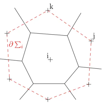
no loss of accuracy. Thegei are computed by the Gauss formula on a neighborhood of

Si, that is the polygonΣi joining the centroids of neighbouring elements (Tomita et al.,

2001). Indeed as

10

Z

V_i

∇f =

Z

∂Σi

(f −f_i)nds, (7)

with∂Σi the boundary ofΣi andnthe outward normal toΣi, we set

e gi=

1

A(Σk)

X

S_i∩S_j∩S_k6=∅

i,j,k distinct



fj+fk

2 −fi



Cj×Ck (8)

where each pair j,k of neighbours appears only once, so that the triangle C_iC_jC_k

is counter-clockwise. In Eq. (8), substracting fi guarantees that a constant field has

15

(7)

GMDD

8, 4979–4996, 2015

E. Kritsikis et al.

Title Page

Tables Figures

◭ ◮

Back Close

Full Screen / Esc

Discussion

P

a

per

|

Discussion

P

a

per

|

Discussion

P

a

per

|

Discussion

P

a

per

|

3 Spherical supermesh

3.1 Intersection between a pair of cells

We describe here how, given two cellsCand C′, their intersection U is obtained. The

unit sphere is represented as the surfacex2+y2+z2=1 in Cartesian coordinates.

In-tersection points between all pairs of edges ofCandC′are computed by representing

5

small and great circles as the intersection of the unit sphere with a plane. For great circles, this plane contains the origin, while it does not for small circles. Among the

resulting segments, those which are inside either C orC′ are collected and ordered

counter-clockwise to form the boundary ofU. Notice thatU is allowed to have several

connected components, in which case as many supermesh cells are created.

10

3.2 Fast search of potential intersectors

Constructing the supermesh requires in principle to compute the intersection between all Si and Tj. Assuming both meshes have O(N) cells, this brute-force approach has

a quadratic algorithmic complexityO(N2). However in fact most intersections are empty. Moreover cells of the source and destination meshes can be grouped hierarchically in

15

sets with mostly empty mutual intersections. Exploiting this fact, as described below, yields fast search algorithms and is crucial to attainO(NlogN) algorithmic complexity.

The fast search algorithm takes as input a mesh and a spherical circle. It yields a list of cells in the mesh that potentially lie partly or totally inside the circle. The algorithm guarantees that all cells of the mesh that actually lie partly or totally in the circle are in

20

the list. Some of those cells may in fact lie outside the circle, although the algorithm is designed to keep their number to a minimum.

In order to yield O(NlogN) complexity, a bounding circle is computed for each

cell and these circles are inserted sequentially into a similarity-search tree, or SS-tree (White and Jain, 1996), which grows progressively starting from an empty SS-tree with

25

(8)

GMDD

8, 4979–4996, 2015

E. Kritsikis et al.

Title Page

Tables Figures

◭ ◮

Back Close

Full Screen / Esc

Discussion

P

a

per

|

Discussion

P

a

per

|

Discussion

P

a

per

|

Discussion

P

a

per

|

circle which encloses the bounding circles of all of its children, and the mesh cells are at the leaves of the tree. To insert one circle, one traverses the tree top-down, choos-ing at each level the closest child node, based on the distance between the centers of the bounding circles. The circle is then inserted at the lowermost level. Before the next circle is inserted, a tree balancing step is performed. If the parent node of the newly

5

inserted cell has more children than a predefined threshold (set here toNmax=10), it

is split in two, hence increasing the child count of its own parent. If the thresholdN_max

is exceeded again, this node is split, and so on until the root node is reached. If the root node needs to be split, a parent node with two children is created and becomes the new root node, increasing the depth of the tree.

10

Every insertion is followed by a re-balancing step in order to avoid a large overlap

between bounding circles, which would diminish the efficiency of the search algorithm

(reference). To this end, after a node (leaf or not) has been inserted, those of its siblings whose distance from the parent exceeds 80 % of its radius are removed from the tree and put into the list of nodes to be inserted later. Such nodes are marked so that they

15

are not removed again from the tree.

To completely specify the tree construction algorithm, we now describe the method used to split a set ofNmax+1 children into two sets. First the child farthest from the

cen-ter of the parent bounding circle is found. Then theNmax/2 nodes closest to that node

are grouped together, while the remaining nodes form another group. Other splitting

20

methods have been proposed and would be easy to implement (refs).

Once all mesh cells have been inserted and the SS-tree is ready, the list of potential intersectors is obtained by traversing the tree top-down, following the branches whose enclosing circle intersects the target circle. The detailed calculation of intersections is performed only with cells in this list.

25

3.3 Connectivity reconstruction

(9)

GMDD

8, 4979–4996, 2015

E. Kritsikis et al.

Title Page

Tables Figures

◭ ◮

Back Close

Full Screen / Esc

Discussion

P

a

per

|

Discussion

P

a

per

|

Discussion

P

a

per

|

Discussion

P

a

per

|

of the meshes. Indeed to reconstruct the connectivity of, say, the source mesh, it is suf-ficient to apply the previous algorithm to the source mesh and a source cell. This con-nectivity is required when computing the gradientge_i. Therefore our method works in cir-cumstances where mesh connectivity is not readily available, for instance when reading data from NetCDF files following the NetCDF-CF convention (http://cfconventions.org/).

5

3.4 Supermesh cell area and barycenter

Supermesh cell edges are an arbitrary mix of small and great circle segments. To compute their area, we represent them as a combination of spherical triangles and surfaces enclosed by a small circle segment and a great circle segment with the same endpoints, possibly counted negatively. A similar approach is used for barycenters.

10

An accurate treatment of small circle segments is crucial for accuracy on reduced latitude–longitude grids (Purser, 1998). Indeed for such grids the cells close to the poles have strongly curved boundaries and approximations that conflate a small arc and the great arc with the same endpoints fail to deliver second-order accuracy (not shown).

15

4 Results

In this section we verify the accuracy and efficiency of the method, encompassing sev-eral types of meshes: latitude–longitude, triangular, polygonal dual and cubed-sphere (see Fig. 2). Computations were done on an Intel P8700 processor @2.53 GHz with 4 GB RAM.

20

4.1 Meshes

(10)

cubed-GMDD

8, 4979–4996, 2015

E. Kritsikis et al.

Title Page

Tables Figures

◭ ◮

Back Close

Full Screen / Esc

Discussion

P

a

per

|

Discussion

P

a

per

|

Discussion

P

a

per

|

Discussion

P

a

per

|

sphere meshes, triangulations and general polygonal meshes. Figure 2 shows meshes that we specifically use for the tests presented below:

– standard longitude–latitude meshes where the zonal and meridional resolution

are equal at the Equator and the pole is a vertex,

– their skipped variant, where the number of cells along a parallel varies, starting

5

at 4 around the pole and doubling to keep the zonal cell size less than twice the meridional cell size (Purser, 1998),

– cubed-sphere meshes (Sadourny, 1972),

– triangular-icosahedral meshes and their hexagonal-pentagonal Voronoi duals

(Sadourny et al., 1968),

10

– variable-resolution variants of the latter obtained by applying a Schmidt transform

to each vertex (Guo and Drake, 2005).

4.2 Accuracy

Interpolation between various pairs of meshes is applied to the smooth field 2+xy.

The input data is obtained by evaluating this function at source cell barycentersG_j. The

15

global conservation property (Eq. 1) is satisfied within round-of error (not shown). Inter-polation error is evaluated by evaluating the test function at destination cell barycenters and comparing to the interpolated valuefj=fj/Aj:

εp=

1 4π

X Aj

fj−f Gj

p1/p

ε_∞=maxj

fj−f Gj

20

(11)

GMDD

8, 4979–4996, 2015

E. Kritsikis et al.

Title Page

Tables Figures

◭ ◮

Back Close

Full Screen / Esc

Discussion

P

a

per

|

Discussion

P

a

per

|

Discussion

P

a

per

|

Discussion

P

a

per

|

the cell size (largest of source and target mesh sizes). When using a piecewise-linear reconstruction, interpolation error is expected to be proportional to the local second derivatives of the test function and to the squared cell size.

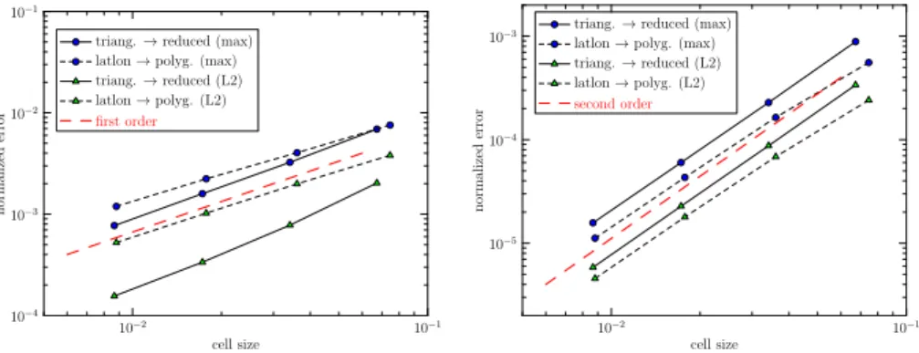
We first consider remapping between pairs of uniform-resolution meshes of

com-parable resolution h ranging from 0.01 (a few hundred thousand cells) to 0.1 (a few

5

thousand cells). Figure 3 shows the maximum (L∞) and root-mean-square (L2)

inter-polation error, as a function of a global characteristic cell sizehdefined as the average of the local cell sizes, themselves defined as the side-length of a square with same areaA (h=p(A)). Scaling of both errors confirms that the expected first order (left) and second-order (right) accuracy is achieved.

10

An application to variable-resolution icosahedral-hexagonal meshes is shown in Fig. 4. The remapping is performed between two such meshes. The source mesh is everywhere about 25 % finer than the destination mesh while the resolution of each sin-gle mesh spans about a decade. As expected, the local error is found to be bounded

O(h2) withhthe local mesh size defined here as the square root of the destination cell

15

area.

4.3 E_fficiency

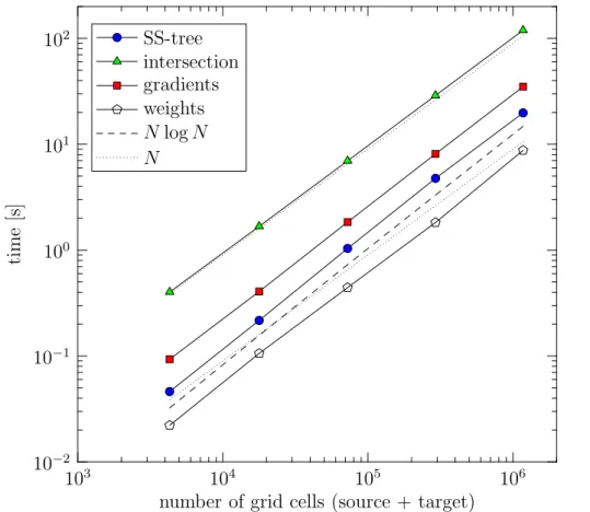
Figure 5 shows the computation time of a second-order remapping from a uniform res-olution icosahedral-hexagonal mesh to a regular latitude–longitude mesh vs. the

num-berN of elements of the meshes. Total time is decomposed according to the different

20

steps of the algorithms. Since the remapping is a linear operator, it can be expressed in terms of weights forming a sparse matrix. These weights are typically pre-computed for repeated later use. The cost of computing intersections, gradients (only for second order) and weights is linear in the number of elements. Construction of the SS-tree has the theoretical complexity ofO(NlogN) (dashed line).

25

(12)

GMDD

8, 4979–4996, 2015

E. Kritsikis et al.

Title Page

Tables Figures

◭ ◮

Back Close

Full Screen / Esc

Discussion

P

a

per

|

Discussion

P

a

per

|

Discussion

P

a

per

|

Discussion

P

a

per

|

problem size the SS-tree will not require more computational resources than the com-putation of intersections, which hasO(N) complexity.

5 Conclusions

A local, explicit, second-order, conservative interpolation algorithm has been devised. The theoretical second-order accuracy has been verified using a smooth test function

5

and pairs of meshes covering most meshes commonly used for atmospheric modelling.

The main efficiency bottleneck caused by the construction of the supermesh has been

overcome by adopting tree-based data structures and algorithms, from which the mesh connectivity can also be deduced efficiently. Experiments confirm aO(NlogN) compu-tational cost of the most expensive operations, especially the supermesh construction.

10

Cartesian curvilinear meshes are not covered by this work. Covering such meshes commonly used for ocean modelling requires essentially adapting the detailed com-putation of intersections. Higher-order interpolations, or vector interpolations can also easily be incorporated. This is left for future work.

Although the present sequential method is fast enough to be included as is into

pre-15

or post-processing pipelines, further efficiency gains can be obtained by parallelizing it. The least parallel part of the algorithm is the SS-tree construction. Work is under way to parallelize this step, using again tree approaches to distribute and balance the workload, and will hopefully be presented separately.

Acknowledgements. E. Kritsikis and M. Aechtner acknowledge support by the ICOMEX project.

20

References

(13)

GMDD

8, 4979–4996, 2015

E. Kritsikis et al.

Title Page

Tables Figures

◭ ◮

Back Close

Full Screen / Esc

Discussion

P

a

per

|

Discussion

P

a

per

|

Discussion

P

a

per

|

Discussion

P

a

per

|

Guo, D. X. and Drake, J. B.: A global semi-Lagrangian spectral model of the shallow water equations with variable resolution, J. Comput. Phys., 206, 559–577, 2005. 4988

Jones, P.: First- and second-order conservative remapping schemes for grids in spherical co-ordinates, Mon. Weather Rev., 127, 2204–2210, 1999. 4981

Purser, R.: Non-standard grids., Proc. Seminar on Recent Developments in Numerical Methods

5

for Atmospheric Modelling, Reading, UK, ECMWF, 44–72, 1998. 4987, 4988

Sadourny, R.: Conservative finite-difference approximations of the primitive equations on quasi-uniform spherical grids, Mon. Weather Rev., 100, 136–144, 1972. 4988

Sadourny, R., Arakawa, A. K. I. O., and Mintz, Y. A. L. E.: Integration of the nondivergent barotropic vorticity equation with an icosahedral-hexagonal grid for the sphere, Mon. Weather

10

Rev., 96, 351–356, 1968. 4988

Tomita, H., Tsugawa, M., Satoh, M., and Goto, K.: Shallow water model on a modified icosahe-dral geodesic grid by using spring dynamics, J. Comput. Phys., 174, 579–613, 2001. 4984 Ullrich, P. A., Lauritzen, P. H., and Jablonowski, C.: Geometrically Exact Conservative

Remap-ping (GECoRe): regular latitude–longitude and cubed-sphere grids, Mon. Weather Rev., 137,

15

1721–1741, 2009. 4981

White, D. and Jain, R.: Similarity indexing with the SS-tree, in: Proceedings of the Twelfth Inter-national Conference on Date of Conference, New Orleans, LA, 26 February–1 March 1996, 516–523, 1996. 4985

Williamson, D. L.: The Evolution of Dynamical Cores for Global Atmospheric Models, J.

Meteo-20

(14)

GMDD

8, 4979–4996, 2015

E. Kritsikis et al.

Title Page

Tables Figures

◭ ◮

Back Close

Full Screen / Esc

Discussion

P

a

per

|

Discussion

P

a

per

|

Discussion

P

a

per

|

Discussion

P

a

per

|

+

i

+

j

+k

+

∂

P

_i

Figure 1.Gradient computation: Stokes formula is applied on the boundary∂Σi of the polygon

(15)

GMDD

8, 4979–4996, 2015

E. Kritsikis et al.

Title Page

Tables Figures

◭ ◮

Back Close

Full Screen / Esc

Discussion

P

a

per

|

Discussion

P

a

per

|

Discussion

P

a

per

|

Discussion

P

a

per

|

(16)

GMDD

8, 4979–4996, 2015

E. Kritsikis et al.

Title Page

Tables Figures

◭ ◮

Back Close

Full Screen / Esc

Discussion

P

a

per

|

Discussion

P

a

per

|

Discussion

P

a

per

|

Discussion

P

a

per

|

10−4

10−3

10−2

10−1

n

or

m

aliz

ed

er

ro

r

10−2

10−1

cell size triang.→reduced (max) latlon→polyg. (max) triang.→reduced (L2) latlon→polyg. (L2)

first order

10−5

10−4

10−3

n

or

m

aliz

ed

er

ro

r

10−2

10−1

cell size triang.→reduced (max) latlon→polyg. (max) triang.→_{reduced (L2)}

latlon→polyg. (L2)

second order

(17)

GMDD

8, 4979–4996, 2015

E. Kritsikis et al.

Title Page

Tables Figures

◭ ◮

Back Close

Full Screen / Esc

Discussion

P

a

per

|

Discussion

P

a

per

|

Discussion

P

a

per

|

Discussion

P

a

per

|

10−8

10−7

10−6

10−5

10−4

lo

ca

l

in

te

rp

ol

at

io

n

er

ro

r

10−2

cell size h

5·10−2

5·10−3

∼h2

(18)

GMDD

8, 4979–4996, 2015

E. Kritsikis et al.

Title Page

Tables Figures

◭ ◮

Back Close

Full Screen / Esc

Discussion

P

a

per

|

Discussion

P

a

per

|

Discussion

P

a

per

|

Discussion

P

a

per

|

10−2

10−1

100

101

102

tim

e

[s

]

103

104

105

106

number of grid cells (source + target) SS-tree

intersection gradients weights N_logN

N