Educational
Data Mining & Students’ Performance
Prediction
Amjad Abu Saa
Information Technology Department Ajman University of Science and Technology
Ajman, United Arab Emirates
Abstract—It is important to study and analyse educational data especially students’ performance. Educational Data Mining (EDM) is the field of study concerned with mining educational data to find out interesting patterns and knowledge in educational organizations. This study is equally concerned with this subject, specifically, the students’ performance. This study explores multiple factors theoretically assumed to affect students’ performance in higher education, and finds a qualitative model which best classifies and predicts the students’ performance based on related personal and social factors.
Keywords—Data Mining; Education; Students; Performance; Patterns
I. INTRODUCTION
Educational Data Mining (EDM) is a new trend in the data mining and Knowledge Discovery in Databases (KDD) field which focuses in mining useful patterns and discovering useful knowledge from the educational information systems, such as, admissions systems, registration systems, course management
systems (moodle, blackboard, etc…), and any other systems
dealing with students at different levels of education, from schools, to colleges and universities. Researchers in this field focus on discovering useful knowledge either to help the educational institutes manage their students better, or to help students to manage their education and deliverables better and enhance their performance.
Analysing students’ data and information to classify students, or to create decision trees or association rules, to
make better decisions or to enhance student’s performance is
an interesting field of research, which mainly focuses on analysing and understanding students’ educational data that indicates their educational performance, and generates specific rules, classifications, and predictions to help students in their future educational performance.
Classification is the most familiar and most effective data mining technique used to classify and predict values. Educational Data Mining (EDM) is no exception of this fact, hence, it was used in this research paper to analyze collected
students’ information through a survey, and provide classifications based on the collected data to predict and
classify students’ performance in their upcoming semester. The objective of this study is to identify relations between students’
personal and social factors, and their academic performance. This newly discovered knowledge can help students as well as instructors in carrying out better enhanced educational quality, by identifying possible underperformers at the beginning of the
semester/year, and apply more attention to them in order to help them in their education process and get better marks. In fact, not only underperformers can benefit from this research, but also possible well performers can benefit from this study by employing more efforts to conduct better projects and research through having more help and attention from their instructors.
There are multiple different classification methods and techniques used in Knowledge Discovery and data mining. Every method or technique has its advantages and disadvantages. Thus, this paper uses multiple classification methods to confirm and verify the results with multiple classifiers. In the end, the best result could be selected in terms of accuracy and precision.
The rest of the paper is structured into 4 sections. In section 2, a review of the related work is presented. Section 3 contains the data mining process implemented in this study, which includes a representation of the collected dataset, an exploration and visualization of the data, and finally the implementation of the data mining tasks and the final results. In section 4, insights about future work are included. Finally, section 5 contains the outcomes of this study.
II. RELATED WORK
Baradwaj and Pal [1] conducted a research on a group of 50 students enrolled in a specific course program across a period of 4 years (2007-2010), with multiple performance indicators,
including “Previous Semester Marks”, “Class Test Grades”, “Seminar Performance”, “Assignments”, “General Proficiency”, “Attendance”, “Lab Work”, and “End Semester Marks”. They used ID3 decision tree algorithm to finally construct a decision tree, and if-then rules which will eventually help the instructors as well as the students to better
understand and predict students’ performance at the end of the
semester. Furthermore, they defined their objective of this
study as: “This study will also work to identify those students
which needed special attention to reduce fail ration and taking
appropriate action for the next semester examination” [1].
Baradwaj and Pal [1] selected ID3 decision tree as their data
mining technique to analyze the students’ performance in the selected course program; because it is a “simple” decision tree learning algorithm.
Abeer and Elaraby [2] conducted a similar research that mainly focuses on generating classification rules and predicting
previously recorded students’ behavior and activities. Abeer
and Elaraby [2] processed and analysed previously enrolled
students’ data in a specific course program across 6 years (2005–10), with multiple attributes collected from the university database. As a result, this study was able to predict, to a certain extent, the students’ final grades in the selected
course program, as well as, “help the student's to improve the student's performance, to identify those students which needed special attention to reduce failing ration and taking appropriate
action at right time” [2].
Pandey and Pal [3] conducted a data mining research using Naïve Bayes classification to analyse, classify, and predict students as performers or underperformers. Naïve Bayes classification is a simple probability classification technique, which assumes that all given attributes in a dataset is
independent from each other, hence the name “Naïve”. Pandey
and Pal [3] conducted this research on a sample data of students enrolled in a Post Graduate Diploma in Computer Applications (PGDCA) in Dr. R. M. L. Awadh University, Faizabad, India. The research was able to classify and predict to a certain extent the students’ grades in their upcoming year, based on their grades in the previous year. Their findings can be employed to help students in their future education in many ways.
Bhardwaj and Pal [4] conducted a significant data mining research using the Naïve Bayes classification method, on a group of BCA students (Bachelor of Computer Applications) in Dr. R. M. L. Awadh University, Faizabad, India, who appeared for the final examination in 2010. A questionnaire was conducted and collected from each student before the final examination, which had multiple personal, social, and psychological questions that was used in the study to identify
relations between these factors and the student’s performance
and grades. Bhardwaj and Pal [4] identified their main
objectives of this study as: “(a) Generation of a data source of
predictive variables; (b) Identification of different factors,
which effects a student’s learning behavior and performance
during academic career; (c) Construction of a prediction model using classification data mining techniques on the basis of identified predictive variables; and (d) Validation of the developed model for higher education students studying in
Indian Universities or Institutions” [4]. They found that the
most influencing factor for student’s performance is his grade in senior secondary school, which tells us, that those students who performed well in their secondary school, will definitely perform well in their Bachelors study. Furthermore, it was found that the living location, medium of teaching, mother’s qualification, student other habits, family annual income, and student family status, all of which, highly contribute in the
students’ educational performance, thus, it can predict a
student’s grade or generally his/her performance if basic personal and social knowledge was collected about him/her.
Yadav, Bhardwaj, and Pal [5] conducted a comparative research to test multiple decision tree algorithms on an educational dataset to classify the educational performance of students. The study mainly focuses on selecting the best decision tree algorithm from among mostly used decision tree algorithms, and provide a benchmark to each one of them. Yadav, Bhardwaj, and Pal [5] found out that the CART
(Classification and Regression Tree) decision tree classification method worked better on the tested dataset, which was selected based on the produced accuracy and precision using 10-fold cross validations. This study presented a good practice of identifying the best classification algorithm technique for a selected dataset; that is by testing multiple algorithms and techniques before deciding which one will eventually work better for the dataset in hand. Hence, it is highly advisable to test the dataset with multiple classifiers first, then choose the most accurate and precise one in order to decide the best classification method for any dataset.
III. DATA MINING PROCESS
The objective of this study is to discover relations between
students’ personal and social factors, and their educational
performance in the previous semester using data mining tasks. Henceforth, their performance could be predicted in the upcoming semesters. Correspondingly, a survey was constructed with multiple personal, social, and academic questions which will later be preprocessed and transformed into nominal data which will be used in the data mining process to find out the relations between the mentioned factors and the students’ performance. The student performance is measured and indicated by the Grade Point Average (GPA), which is a real number out of 4.0. This study was conducted on a group of students enrolled in different colleges in Ajman University of Science and Technology (AUST), Ajman, United Arab Emirates.
A. Dataset
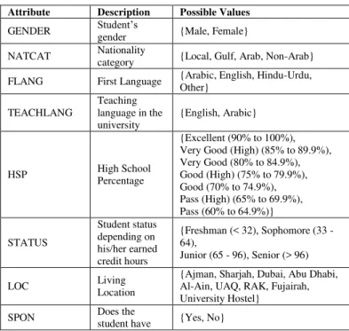
The dataset used in this study was collected through a survey distributed to different students within their daily classes and as an online survey using Google Forms, the data was collected anonymously and without any bias. The initial size of the dataset is 270 records. Table 1 describes the attributes of the data and their possible values.
TABLE I. ATTRIBUTES DESCRIPTION AND POSSIBLE VALUES
Attribute Description Possible Values
GENDER Student’s
gender {Male, Female}
NATCAT Nationality
category {Local, Gulf, Arab, Non-Arab}
FLANG First Language {Arabic, English, Hindu-Urdu, Other}
TEACHLANG
Teaching language in the university
{English, Arabic}
HSP High School Percentage
{Excellent (90% to 100%), Very Good (High) (85% to 89.9%), Very Good (80% to 84.9%), Good (High) (75% to 79.9%), Good (70% to 74.9%), Pass (High) (65% to 69.9%), Pass (60% to 64.9%)}
STATUS
Student status depending on his/her earned credit hours
{Freshman (< 32), Sophomore (33 - 64),
Junior (65 - 96), Senior (> 96)
LOC Living
Location
{Ajman, Sharjah, Dubai, Abu Dhabi, Al-Ain, UAQ, RAK, Fujairah, University Hostel}
SPON Does the
any sponsorship
PWIU
Any parent works in the university
{Yes, No}
DISCOUNT Student
discounts {Yes, No}
TRANSPORT
How the student comes to the university
{Private car, Public Transport, University Bus, Walking}
FAMSIZE Family Size {Single, With one parent, With both parents, medium family, big family}
INCOME
Total Family Monthly Income
{Low, Medium, Above Medium, High}
PARSTATUS Parents Marital Status
{Married, Divorced, Separated, Widowed}
FQUAL Father’s Qualifications
{No Education, Elementary, Secondary, Graduate, Post Graduate, Doctorate, N/A}
MQUAL Mother’s Qualifications
{No Education, Elementary, Secondary, Graduate, Post Graduate, Doctorate, N/A}
FOCS
Father’s Occupation Status
{Currently on Service, Retired, In between Jobs, N/A}
MOCS
Mother’s Occupation Status
{Currently on Service, Retired, In between Jobs, Housewife, N/A}
FRIENDS Number of Friends
{None, One, Average, Medium, Above Medium, High}
WEEKHOURS
Average number of hours spent with friends per week
{None, Very limited, Average, Medium, High, Very High}
GPA Previous Semester GPA
{> 3.60 (Excellent), 3.00 – 3.59 (Very Good), 2.50 – 2.99 (Good), < 2.5 – (Pass)}
Following is a more detailed description about some attributes mentioned in Table 1:
TEACHLANG: Some majors in the university are taught in English, and some others are taught in Arabic, and hence, it is useful to know the teaching language of the student, as it might be linked with his/her performance.
STATUS: The University follows the American credit hours system, and hence, the status of the student can be acquired from his/her completed/earned credit hours. FAMSIZE: The possible values of this attribute are
derived from the questionnaire as: 1 is “Single”, 2 is “With one parent”, 3 is “With both parents”, 4 is “medium family”, and 5 and above is “big family”. INCOME: The possible values of this attribute are
derived from the questionnaire as: < AED 15,000 is
“Low”, AED 15,000 to 25,000 is “Medium”, AED 25,000 to 50,000 is “Above Medium”, and above 50,000 is “High”.
FRIENDS: The possible values of this attribute are derived from the questionnaire as: None is “None”, 1 is
“One”, 2 to 5 is “Average”, 6 to 10 is “Medium”, 11 to 15 is “Above Medium”, and above 15 is “High”. WEEKHOURS: The possible values of this attribute are
derived from the questionnaire as: None is “None”, 1 to 2 hours is “Very limited”, 2 to 10 hours is “Average”, 10 to 20 hours is “Medium”, 20 to 30 hours is “High”, and more than 30 hours is “Very High.
B. Data Exploration
In order to understand the dataset in hand, it must be explored in a statistical manner, as well as, visualize it using graphical plots and diagrams. This step in data mining is essential because it allows the researchers as well as the readers to understand the data before jumping into applying more complex data mining tasks and algorithms.
Table 2 shows the ranges of the data in the dataset according to their attributes, ordered from highest to lowest.
TABLE II. RANGES OF DATA IN THE DATASET
Attribute Range
GPA Very Good (81), Good (68), Pass (61), Excellent (60) GENDER Female (174), Male (96)
STATUS Freshman (109), Sophomore (62), Junior (53), Senior (37)
NATCAT Arab (180), Other (34), Gulf (29), Local (23), Non-Arab (4)
FLANG Arabic (233), Other (18), Hindi-Urdu (16), English (3) TEACHLANG English (248), Arabic (20)
LOC
Ajman (123), Sharjah (90), Dubai (18), University Hostel (13), RAK (11),
UAQ (10), Abu Dhabi (3), Fujairah (1), Al-Ain (1)
TRANSPORT Car (175), University Bus (54), Walking (21), Public Transport (20)
HSP
Excellent (100), Very Good (High) (63), Very Good (50),
Good (High) (33), Good (19), Pass (High) (4), Pass (1) PWIU No (262), Yes (8)
DISCOUNT No (186), Yes (84) SPON No (210), Yes (60)
FRIENDS Average (81), High (75), Medium (67), Above Medium (27), One (13), None (7)
WEEKHOURS Average (122), Very limited (57), Medium (40), High (21), Very High (16), None (14)
FAMSIZE Big (232), Medium (28), With both parents (6), With Two Parents (1), Single (1)
INCOME Medium (83), Low (70), Above Medium (54), High (27)
PARSTATUS Married (243), Widowed (17), Separated (6), Divorced (4)
FQUAL
Graduate (144), Post Graduate (41), Secondary (37), Doctorate (20), Elementary (11), N/A (10), No Education (7)
MQUAL
Graduate (140), Secondary (60), Post Graduate (25), No Education (16), Elementary (11), Doctorate (9), N/A (8)
FOCS Service (166), N/A (42), Retired (32), In Between Jobs (30)
MOCS Housewife (162), Service (65), N/A (22), In Between Jobs (11), Retired (10)
TABLE III. SUMMARY STATISTICS
Attribute Mode Least Missing Values
GPA Very Good (81) Excellent (30) 0 GENDER Female (174) Male (96) 0 STATUS Freshman (109) Senior (37) 9 NATCAT Arab (180) Non-Arab (4) 0 FLANG Arabic (233) English (3) 0 TEACHLANG English (248) Arabic (20) 2 LOC Ajman (123) Fujairah (1) 0
TRANSPORT Car (175) Public Transport (20) 0
HSP Excellent (100) Pass (1) 0
PWIU No (262) Yes (8) 0
DISCOUNT No (186) Yes (84) 0
SPON No (210) Yes (60) 0
FRIENDS Average (81) None (7) 0 WEEKHOURS Average (122) None (14) 0
FAMSIZE Big (232) With Two Parents
(1) 2
INCOME Medium (83) High (27) 36 PARSTATUS Married (243) Divorced (4) 0 FQUAL Graduate (144) No Education (7) 0 MQUAL Graduate (140) N/A (8) 1
FOCS Service (166) In Between Jobs
(30) 0
MOCS Housewife (162) Retired (10) 0
Fig. 1. Histogram of GPA attribute
Fig. 2. Histogram of TRANSPORT attribute
Fig. 3. Histogram of HSP attribute
Fig. 4. Histogram of WEEKHOURS attribute
It is equally important to plot the data in graphical visualizations in order to understand the data, its characteristics, and its relationships. Henceforth, figures 1 to 4 are constructed as graphical plots of the data based on the summary statistics.
C. Data Mining Implementation & Results
There are multiple well known techniques available for data mining and knowledge discovery in databases (KDD), such as Classification, Clustering, Association Rule Learning, Artificial Intelligence, etc.
Classification is one of the mostly used and studied data mining technique. Researchers use and study classification because it is simple and easy to use. In detail, in data mining,
Classification is a technique for predicting a data object’s class
or category based on previously learned classes from a training dataset, where the classes of the objects are known. There are multiple classification techniques available in data mining, such as, Decision Trees, K-Nearest Neighbor (K-NN), Neural Networks, Naïve Bayes, etc.
0 20 40 60 80 100
Excellent Very Good Good Pass
GPA
GPA
0 20 40 60 80 100 120 140 160 180 200
Car University Bus
Walking Public Transport
TRANSPORT
TRANSPORT
0 20 40 60 80 100 120
HSP
HSP
0 20 40 60 80 100 120 140
None Very Limited
Average Medium High Very High
WEEKHOURS
In this study, multiple classification techniques was used in the data mining process for predicting the students’ grade at the end of the semester. This approach was used because it can provide a broader look and understanding of the final results and output, as well as, it will lead to a comparative conclusion over the outcomes of the study. Furthermore, a 10-fold cross validation was used to verify and validate the outcomes of the used algorithms and provide accuracy and precision measures.
All data mining implementation and processing in this study was done using RapidMiner and WEKA.
As can be seen from Table 3 in the previous section (3.2),
the mode of the class attribute (GPA) is “Very Good”, which
occurs 81 times or 30% in the dataset. And hence, this percentage can be used as a reference to the accuracy measures produced by the algorithms in this section. Notably, in data mining, this is called the default model accuracy. The default model is a naïve model that predicts the classes of all examples in a dataset as the class of its mode (highest frequency). For
example, let’s consider a dataset of 100 records and 2 classes (Yes & No), the “Yes” occurs 75 times and “No” occurs 25
times, the default model for this dataset will classify all objects
as “Yes”, hence, its accuracy will be 75%. Even though it is useless, but equally important, it allows to evaluate the accuracies produced by other classification models. This concept can be generalized to all classes/labels in the data to produce an expectation of the class recall as well. Henceforth, Table 4 was constructed to summarize the expected recall for each class in the dataset.
TABLE IV. EXPECTED RECALL
Class (Label) Excellent Very Good Good Pass
Expected Recall 22.2% 30.0% 25.2% 22.6% 1) Decision Tree Induction
A decision tree is a supervised classification technique that builds a top-down tree-like model from a given dataset attributes. The decision tree is a predictive modeling technique used for predicting, classifying, or categorizing a given data object based on the previously generated model using a training dataset with the same features (attributes). The structure of the generated tree includes a root node, internal nodes, and leaf (terminal) nodes. The root node is the first node in the decision tree which have no incoming edges, and one or more outgoing edges; an internal node is a middle node in the decision tree which have one incoming edge, and one or more outgoing edges; the leaf node is the last node in the decision tree structure which represents the final suggested (predicted) class (label) of a data object.
In this study, four decision tree algorithms was used on the
collected student’s data, namely, C4.5 decision tree, ID3
decision tree, CART decision Tree, and CHAID. C4.5 Decision Tree
The C4.5 decision tree algorithm is an algorithm developed by Ross Quinlan, which was the successor of the ID3 algorithm. The C4.5 algorithm uses pruning in the generation of a decision tree, where a node could be removed from the tree if it adds little to no value to the final predictive model.
Furthermore, the following settings was used with the C4.5 operator to produce the decision tree.
Splitting criterion = information gain ratio Minimal size of split = 4
Minimal leaf size = 1 Minimal gain = 0.1 Maximal depth = 20 Confidence = 0.5
After running the C4.5 decision tree algorithm with the 10-fold cross validation on dataset, the following confusion matrix was generated.
Actual Class Precision (%) Excellent Very
Good Good Pass
Pr
e
d
ic
ti
o
n
Excellent 23 12 8 6 46.94
Very Good 20 40 30 29 33.61
Good 11 10 18 12 35.29
Pass 6 19 12 14 27.45
Class Recall (%) 38.33 49.38 26.47 22.95
The C4.5 algorithm was able to predict the class of 95 objects out of 270, which gives it an Accuracy value of 35.19%.
ID3 Decision Tree
The ID3 (Iterative Dichotomiser 3) decision tree algorithm is an algorithm developed by Ross Quinlan. The algorithm generates an unpruned full decision tree from a dataset.
Following are the settings used with the ID3 operator to produce the decision tree.
Splitting criterion = information gain ratio Minimal size of split = 4
Minimal leaf size = 1 Minimal gain = 0.1
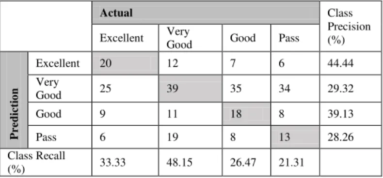
After running the ID3 decision tree algorithm with the 10-fold cross validation on the dataset, the following confusion matrix was generated.
Actual Class Precision (%) Excellent Very
Good Good Pass
Pr
e
d
ic
ti
o
n
Excellent 20 12 7 6 44.44
Very
Good 25 39 35 34 29.32
Good 9 11 18 8 39.13
Pass 6 19 8 13 28.26
Class Recall
The ID3 algorithm was able to predict the class of 90 objects out of 270, which gives it an Accuracy value of 33.33%.
CART Decision Tree
Classification and Regression Tree (CART) is another decision tree algorithm which uses minimal cost-complexity pruning.
Following are the settings used with the CART operator to produce the decision tree:
Minimal leaf size = 1
Number of folds used in minimal cost-complexity pruning = 5
After running the CART algorithm with the 10-fold cross validation on the dataset, the following confusion matrix was generated.
Actual Class Precision (%) Excellent Very
Good Good Pass
Pr
e
d
ic
ti
o
n
Excellent 43 16 10 6 57.33
Very
Good 12 40 38 26 34.48
Good 4 10 2 6 9.09
Pass 1 15 18 23 40.35
Class Recall (%) 71.67 49.38 2.94 37.70
CART algorithm was able to predict the class of 108 objects out of 270, which gives it an Accuracy value of 40%.
CHAID Decision Tree
CHi-squared Automatic Interaction Detection (CHAID) is another decision tree algorithm which uses chi-squared based splitting criterion instead of the usual splitting criterions used in other decision tree algorithms.
Following are the settings used with the CART operator to produce the decision tree.
Minimal size of split = 4 Minimal leaf size = 2 Minimal gain = 0.1 Maximal depth = 20 Confidence = 0.5
After running the CHAID algorithm with the 10-fold cross validation on the dataset, the following confusion matrix was generated:
Actual Class Precision (%) Excellent Very
Good Good Pass
Pr
e
d
ic
ti
o
n
Excellent 16 14 5 5 40.00
Very
Good 23 36 31 25 31.30
Good 9 11 17 8 37.78
Pass 12 20 15 23 32.86
Class Recall (%) 26.67 44.44 25.00 37.70
The CHAID algorithm was able to predict the class of 92 objects out of 270, which gives it an Accuracy value of 34.07%.
Analysis and Summary
In this section, multiple decision tree techniques and algorithms were reviewed, and their performances and accuracies were tested and validated. As a final analysis, it was obviously noticed that some algorithms worked better with the dataset than others, in detail, CART had the best accuracy of 40%, which was significantly more than the expected (default model) accuracy, CHAID and C4.5 was next with 34.07% and 35.19% respectively, and the least accurate was ID3 with 33.33%. On the other hand, it was noticeable that the class recalls was always higher than the expectations assumed in Table 4, which some might argue with. Furthermore, it have been seen that most of the algorithms have struggled in distinguishing similar classes objects, and as a result, multiple objects was noticed being classified to their nearest similar class; for example, let’s consider the class “Good” in the CART confusion matrix, it can be seen that 38 objects (out of
68) was classified as “Very Good”, which is considered as the
upper nearest class in terms of grades, similarly, 18 objects was
classified as “Pass” which is also considered as the lower
nearest class in terms of grades. This observation leads to conclude that the discretization of the class attribute was not suitable enough to capture the differences in other attributes, or, the attributes themselves was not clear enough to capture such differences, in other words, the classes used in this research was not totally independent, for instance, an
“Excellent” student can have the same characteristics
(attributes) as a “Very Good” student, and hence, this can
confuse the classification algorithm and have big effects on its performance and accuracy.
2) Naïve Bayes Classification
Naïve Bayes classification is a simple probability classification technique, which assumes that all given attributes in a dataset is independent from each other, hence the name
“Bayes classification has been proposed that is based on
Bayes rule of conditional probability. Bayes rule is a technique to estimate the likelihood of a property given the set of data as
evidence or input Bayes rule or Bayes theorem is” [4]:
In order to summarize the probability distribution matrix generated by the Bayes model, the mode class attributes which have probabilities greater than 0.5 was selected. The selected rows are shown in Table 5.
TABLE V. PROBABILITY DISTRIBUTION MATRIX
Attribute Value
Probability Excellent Very
Good Good Pass
TEACHLANG English 0.883 0.975 0.882 0.918 PWIU No 0.950 0.963 0.971 1.000 PARSTATUS Married 0.900 0.938 0.897 0.852 FAMSIZE Big 0.800 0.877 0.897 0.852 FLANG Arabic 0.833 0.802 0.912 0.918 DISCOUNT No 0.250 0.778 0.838 0.836 SPON No 0.867 0.753 0.721 0.787 GENDER Female 0.733 0.691 0.676 0.459 NATCAT Arab 0.683 0.630 0.647 0.721 TRANSPORT Car 0.600 0.630 0.691 0.672 FOCS Service 0.650 0.630 0.559 0.623 FQUAL Graduate 0.550 0.580 0.456 0.541 MOCS Housewife 0.550 0.580 0.574 0.705 MQUAL Graduate 0.550 0.531 0.515 0.475 WEEKHOURS Average 0.483 0.519 0.456 0.328
After the generation of the Bayes probability distribution matrix, in order to distinguish interesting probabilities from not interesting ones, a function was constructed to do that. The
function calculates the absolute difference between the classes’
probabilities for each row in the confusion matrix, and only if the absolute difference between two of them is more than 0.25 (25%), it will be considered as interesting, as well as, attributes with one or more class probability greater than or equal 0.35
(35%) was considered. Let’s take an example to better clarify the idea; let’s consider the following two rows from the
generated confusion matrix.
Row Attribute Value
Probability
Interesting
Excel-lent Very
Good Good Pass
1 DISCOUNT Yes 0.750 0.222 0.162 0.164 Interesting
2 TEACHLANG English 0.883 0.975 0.882 0.918 Not Interesting
It can be seen that row 1 was considered as interesting because there are 2 probabilities greater than 0.35, and the absolute difference between some pairs of probability values are more than 0.25 (25%), hence, it is marked as interesting. Significantly, the interestingness behind the first row is that the
probability of an “Honors” student to have a discount
(value=Yes) is 86.7%, and it gets lower when it moves down to less GPA classes; Excellent 63.3%, Very Good 22.2%, etc... Furthermore, row 2 is considered not interesting because there are not much difference between the probabilities between the classes, even though they have high probabilities, henceforth, this attribute had almost the same probability across all types (classes) of students. Likewise, Table 6 shows all interesting probabilities found in the Bayes distribution matrix.
TABLE VI. INTERESTING BAYES PROBABILITIES
Row Attribute Value Probability
Excellent Very Good Good Pass
1
GENDER Female 0.733 0.691 0.676 0.459 2 Male 0.267 0.309 0.324 0.541 3 HSP Excellent 0.683 0.407 0.279 0.115 4 MOCS Service 0.350 0.247 0.235 0.131 5
DISCOUNT No 0.250 0.778 0.838 0.836
6 Yes 0.750 0.222 0.162 0.164
Following are the description for each one of the interesting Bayes Probabilities:
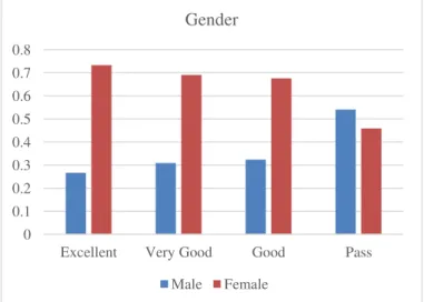
a)GENDER = Male: The probability of male students to get lower grades are significantly higher. Moving from higher to lower grades, the probability increases.
b)GENDER = Female: This scenario is opposite to the previous one, where the probability of female students to get higher grades are significantly higher. The probability decreases moving from high to low grades.
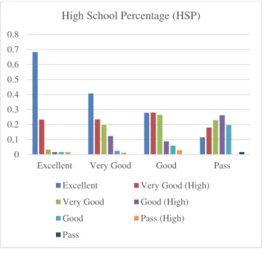
c)HSP = Excellent: Interesting enough, students who got excellent grades in High School had high grades in the university as well.
d)MOCS = Service: Interestingly, when the mother occupation status is on service, it appears that students get higher grades.
e)DISCOUNT: As illustrated earlier, students with higher grades tend to get discounts from the university more than low grades students.
Fig. 5. Interesting probabilities of GENDER 0
0.1 0.2 0.3 0.4 0.5 0.6 0.7 0.8
Excellent Very Good Good Pass
Gender
Fig. 6. Interesting probabilities of HSP
Fig. 7. Interesting probabilities of MOCS
Fig. 8. Interesting probabilities of DISCOUNT
Following is the confusion matrix of the Naïve Bayes classification model performance generated by the 10-fold cross validation:
Actual
Class Precision (%) Excellent Very
Good Good Pass
Pr
e
d
ic
ti
o
n
Excellent 29 15 9 5 50.00
Very
Good 16 27 26 16 31.76
Good 5 27 16 16 25.00
Pass 5 11 14 23 43.40
Class Recall
(%) 52.73 33.75 24.62 38.33
The Naïve Bayes classifier was able to predict the class of 95 objects out of 270, which gives it an Accuracy value of 36.40%.
Analysis and Summary
In this section, a review of the implementation of the Naïve Bayes classification technique was presented on the dataset used in this research, as well as, its performance and accuracy have been tested and validated. Furthermore, this section has suggested some techniques to find interesting patterns in the Naïve Bayes model. As a final analysis, this section presented high potential results in the data mining analysis of the Naïve Bayes model, as well as, more interesting patterns could be drawn in the future from the Naïve Bayes model using other techniques.
IV. CONCLUSION
In this research paper, multiple data mining tasks were used to create qualitative predictive models which were efficiently
and effectively able to predict the students’ grades from a
collected training dataset. First, a survey was constructed that has targeted university students and collected multiple personal, social, and academic data related to them. Second, the collected dataset was preprocessed and explored to become appropriate for the data mining tasks. Third, the implementation of data mining tasks was presented on the dataset in hand to generate classification models and testing them. Finally, interesting results were drawn from the classification models, as well as, interesting patterns in the Naïve Bayes model was found. Four decision tree algorithms have been implemented, as well as, with the Naïve Bayes algorithm. In the current study, it was slightly found that the
student’s performance is not totally dependent on their
academic efforts, in spite, there are many other factors that have equal to greater influences as well. In conclusion, this study can motivate and help universities to perform data
mining tasks on their students’ data regularly to find out
interesting results and patterns which can help both the university as well as the students in many ways.
V. FUTURE WORK
Using the same dataset, it would be possible to do more data mining tasks on it, as well as, apply more algorithms. For the time being, it would be interesting to apply association rules mining to find out interesting rules in the students data. 0
0.1 0.2 0.3 0.4 0.5 0.6 0.7 0.8
Excellent Very Good Good Pass
High School Percentage (HSP)
Excellent Very Good (High)
Very Good Good (High)
Good Pass (High)
Pass
0 0.1 0.2 0.3 0.4 0.5 0.6 0.7 0.8
Excellent Very Good Good Pass
Mother Occupation Status (MOCS)
Service Housewife Retired In Between Jobs N/A
0 0.2 0.4 0.6 0.8 1
Excellent Very Good Good Pass
Discount
Similarly, clustering would be another data mining task that
could be interesting to apply. Moreover, the students’ data that
was collected in this research included a classic sampling process which was a time consuming task, it could be better if the data was collected as part of the admission process of the university, that way, it would be easier to collect the data, as well as, the dataset would have been much bigger, and the university could run these data mining tasks regularly on their students to find out interesting patterns and maybe improve their performance.
ACKNOWLEDGMENT
I would like to express my very great appreciation to Dr Sherief Abdallah, Associate Professor, British University in Dubai, for his valuable efforts in teaching me data mining and exploration module in my Masters study, as well as, for his valuable and constructive suggestions and overall help in conducting this research.
I would also like to thank Dr. Ahmed Ankit, Assistant to the President, Ajman University of Science and Technology, and Mrs Inas Abou Sharkh, IT Manager, Ajman University of Science and Technology, for their great support during the planning and development of this research work, and for allowing me to conduct this research on the university campus.
As well as, I would like to thank and express my very great appreciation to Dr Mirna Nachouki, Assistant Professor and Head of Department, Information Systems Department, College of IT, Ajman University of Science and Technology, for her great support and inspiration during the whole time of conducting this research, as well as, her willingness to allocate her time so generously, along with:
Mrs Amina Abou Sharkh, Teaching Assistant, Information Systems Department, College of IT, Ajman University of Science and Technology.
Mr Hassan Sahyoun, Lecturer, Information Systems Department, College of IT, Ajman University of Science and Technology.
Last but not least, I would like to thank my wife, and my family for continuously supporting and inspiring me during my study and research.
REFERENCES
[1] Baradwaj, B.K. and Pal, S., 2011. Mining Educational Data to Analyze Students’ Performance. (IJACSA) International Journal of Advanced Computer Science and Applications, Vol. 2, No. 6, 2011.
[2] Ahmed, A.B.E.D. and Elaraby, I.S., 2014. Data Mining: A prediction for Student's Performance Using Classification Method. World Journal of Computer Application and Technology, 2(2), pp.43-47.
[3] Pandey, U.K. and Pal, S., 2011. Data Mining: A prediction of performer or underperformer using classification. (IJCSIT) International Journal of Computer Science and Information Technologies, Vol. 2 (2), 2011, 686-690.
[4] Bhardwaj, B.K. and Pal, S., 2012. Data Mining: A prediction for performance improvement using classification. (IJCSIS) International Journal of Computer Science and Information Security, Vol. 9, No. 4, April 2011.
[5] Yadav, S.K., Bharadwaj, B. and Pal, S., 2012. Data Mining Applications: A Comparative Study for Predicting Student’s Performance. International Journal of Innovative Technology & Creative Engineering (ISSN: 2045-711), Vol. 1, No.12, December.