Performance Evaluation of Spatial Vector Routing Protocol for Wireless Sensor Networks

Wireless Sensor Networks

JAVED ALI BALOCH*, IMRAN ALI JOKHIO**, AND SANA HOOR JOKHIO*

RECIEVED ON 24.12.2011 ACCEPTED ON 21.06.2012

ABSTRACT

WSNs (Wireless Sensor Networks) is an emerging area of research. Researchers worldwide are working on the issues faced by sensor nodes. Communication has been a major issue in wireless networks and the problem is manifolds in WSNs because of the limited resources. The routing protocol in such networks plays a pivotal role, as an effective routing protocol could significantly reduce the energy consumed in transmitting and receiving data packets throughout a network. In this paper the performance of SVR (Spatial Vector Routing) an energy efficient, location aware routing protocol is compared with the existing location aware protocols. The results from the simulation trials show the performance of SVR.

Key Words: Wireless Sensor Networks, SVR, LAR, DREAM, GPSR, Routing Protocols

* Assistant Professor, Department of Computer Systems Engineering, Mehran University of Engineering & Technology, Jamshoro. * * Assistant Professor, Department of Software Engineering, Mehran University of Engineering & Technology, Jamshoro.

1.

INTRODUCTION

energy efficiency and different protocols address diverse

methodologies which could be adapted to accomplish this

major goal. Some of the techniques could be to reduce

data redundancy, decrease processing, route data with

smaller hops, etc.

The characteristics of WSNs set them apart from the

classical wired and wireless networks, as there are much

more constraints associated with them. In order for a

routing protocol to work effectively in a WSN the

design of the protocol will play a major role, as there are

many concerns regarding wireless sensor networks,

which need to be kept in mind while designing a routing

protocol for WSNs. The most important ones are

mentioned below.

W

classified as adhoc networks. WSNs are

considered as energy constrained and with less bandwidth

supply because of the wireless medium [1-3]. With

advancements in technology it is now possible to design

sensor nodes of miniature size. The reduced size of sensor

nodes introduce many new challenges such as reduced

memory, processing capabilities and battery energy, which

have to be addressed. To address these challenges there

is a need of energy efficient schemes, which reduce the

communication costs.

Routing protocols designed specifically for such networks

„ Data-Centric: Wireless sensor networks are data-centric in nature and they have the ability to deal with specific queries which could be generated while the sensor nodes are performing their sensing tasks or these queries could instigate certain tasks. For example if the temperature rises to 40o_{C then send an alert}

throughout the network that it is extremely hot.

„ Application Specific: WSNs are application specific networks. Routing protocols have to be tailored for the specific application.

„ Node Deployment: Nodes of a WSN may be deployed in a regular uniform fashion but in most networks they are deployed randomly, such as deploying a network by scattering nodes from a plane. Sensor nodes have the ability to form a network, as they are self-configurable.

„ Prone to Failure: Some sensor nodes may deplete their energy earlier than others depending on their task load, it is nontrivial for the routing protocols to have the ability to reroute.

„ Scalability: WSNs have a large number of nodes, in hundreds or even thousand and as each node has limited processing, memory and battery storage; the nodes need to communicate with each other to achieve greater accuracy and carry out complex tasks.

„ Less Mobility: Sensor nodes are usually fixed but in some cases nodes could be mobile as well, although their movement is comparatively less as compared to other networks.

„ Quality of Service: Increased network life time is one of the main priorities of WSNs which could be achieved by a trade off with the quality of service such as the sensor nodes may increase the time interval between every time it senses the phenomena, this could be done when the battery life of a node goes low.

In this paper existing location aware protocols are compared in terms of energy consumption of sensor nodes and the effect of different location aware routing protocols on a networks lifetime is investigated. As sensor nodes are usually deployed randomly, in this paper a random deployment is considered and apart from that a uniform deployment of sensor nodes is also considered. The results of simulation trials show the performance of some of the most common location aware protocols.

In the paper the introduction is followed by location aware routing protocols section. This section gives a brief idea of location aware routing protocols and how the network could benefit from location information. In Section 3 the working of Spatial Vector Routing protocol is explained. Sections 4-6 explain the functionality of Location aided routing, Distance Routing Effect Algorithm for Mobility and Greedy Perimeter Stateless Routing respectively. The protocol description is followed by simulation setup in Section 6, which describes the simulation environment. Section 7 includes the results obtained through the simulation trials and finally the paper is concluded in Section 8.

2.

LOCATION AWARE ROUTING

PROTOCOLS

WSNs could perform smart tasks when provided with location information. With nodes knowing their own location each node could keep track of its neighboring nodes. Location aware routing protocols play a vital role in WSNs, as knowing a nodes location could substantially reduce data redundancy and result in minimizing the energy consumption of a node while communicating with other nodes.

most cases, but depending on the type of application at times semantic representation of location is required like building, floor, room, etc. WSNs could greatly benefit from the use of location aware routing protocols in various network scenarios including:

† Networks comprising of mobile nodes.

† Networks where nodes need to be self configurable.

† Networks where route discovery is frequent.

Among the existing location aware routing protocols, the selection of the protocols to compare with Spatial Vector Routing protocol was made on the mechanism each protocol uses to route data. LAR protocol works on a request zone and expected zone, DREAM makes use of a location table to store the location of the nodes, and GPSR uses a directional approach. Each protocols technique varies from the other. The SVR protocol and the location aware protocols compared with it are discussed in detail in the following sections.

3.

SPATIAL VECTOR ROUTING

PROTOCOL

SVR protocol[4,5] is a data centric protocol for wireless sensor networks. SVR uses a distributed approach to work in sensor networks, which are spatially aware. SVR exploits the nodes position in the network to reduce data redundancy and conserve energy while performing smart tasks. The SVR protocol aims to enable inter-node cooperation within the nodes of a sensor network, which could attribute towards the smart behavior of the network. SVR varies from the Ad hoc routing protocols in nature as it is a data centric routing protocol targeted for WSNs where tasks are complicated and most of them are event driven and even query based. Although Ad hoc network routing protocols serve as a stepping stone for WSN routing protocols they differ many-folds from the WSN protocols with their high criticality.

SVR assumes that sensor nodes are aware of their position, which could be easily obtained by GPS and other

well established localization techniques. The position of neighboring nodes could then be discovered easily as each node has a limited range (radio range of sensor nodes). In order to route data packets location information is provided, as mentioned earlier on. SVR is a location aware protocol, which benefits from the nodes position in a network. Header of the packets generated include location information i.e. the x,y coordinates of the destination node (target node). The destination nodes location information makes it possible to route the data packet in the right direction. Knowing the location of the nodes it reduces data redundancy as a message is only sent once by one node until it reaches the destination node, which provides increased efficiency as compared to flooding. Once a query is generated or a task is assigned to a node it needs to follow certain steps to forward data throughout the network, the four main steps are mentioned below.

♦ Proximate Node (Pn): Once the spatial vector communication process is started each node discovers its proximate nodes. Proximate nodes are the neighboring nodes of a node, that is nodes that are in the communication range.

♦ Bearing Angle (Ba): The angle between the source node and the destination node is computed, followed by the computation of the bearing angle between the proximate nodes and the destination node.

♦ Optimal Proximate Node (OPn): On knowing the bearing angle the proximate node in nearest direction to the destination nodes is chosen as the optimal proximate node. The data packet is then forwarded to the optimal proximate node from the source node.

4.

LOCATION AIDED ROUTING

LAR (Location Aided Routing) [6] protocol exploits the location information of nodes to reduce the routing overhead. LAR demonstrates how routing based on flooding could be improved significantly with location information. A simple example of flooding could be considered where a Source node Sn sends a message m to a Destination node Dn. In the case of flooding the source node would flood the message to all its neighbors and each node would do so until the message reaches the destination. Even though redundant messages could be discarded, flooding would be highly energy consuming and impractical if the nodes were mobile.

LAR protocol assumes the nodes know their location, which could be easily calculated with a GPS receiver. Nodes knowing their location could estimate the position of mobile nodes. To compute mobile nodes position their position should be known at a certain time and the speed at which they are moving. LAR protocol introduces the concept of Expected Zones and Requested Zones, which reduce the flooding and are effective with mobile nodes. The region in which a node is likely to be in a specific time frame is known as the expected zone, when the initial position of the node and the speed with which it is moving are known. The region in which the expected zone is present along with some surrounding area is known as the request zone. The concept of creating these zones is to reduce flooding within the network. When a source node requests for a route, a message is propagated in the request zone. If a route is not found then the message is discarded and the requested zone is expanded for the next route discovery. When accurate information of the nodes direction is known the expected zone size could be reduced. Two schemes of LAR have been proposed. The request zone in scheme one comprises of the shortest rectangular area, which contains the originating node and the expected zone (which is normally a circle). While in scheme two when the originating node forwards a route request only the nodes nearest to the final node than the originating node forward the message, and the other nodes would simply dump it.

5.

DREAM

The DREAM (Distance Routing Effect Algorithm for

Mobility) [7] differs from other routing algorithm, which maintain routing tables. The inclusion of a location table for each node makes routing easier. DREAM uses the

location table of each node, not only to calculate the distance of each node, but also to find the direction of a

node. If a Source node Sn needs to forward message m to a Destination node Dn it will send the message to its neighboring nodes in the direction of Dn. This method

reduces the number of messages being sent and has an overall impact on the network lifetime.

To achieve energy efficient communication, the DREAM protocol is required to reduce the location information

dissipation throughout the network. The location information dissipation depends on how frequently the location table is updated. The protocol introduces control packets, which determine the distance effect and the

mobility rate. Each node transmits a control packet with a specified lifetime. Some packets may have shorter lifetime, while other packets may have longer lifetime. The distance

traveled by a control packet from the originating node depends on the lifetime, the greater the lifetime the greater the distance it covers. The measure of the distance traveled by such packets from the source towards a destination would be a deciding factor on how often the table should

be updated.

The location table is updated on two principles: the distance effect and the mobility rate. As the principles

name infers, the distance effect demonstrates the effect of distance between two nodes. The updating of the location table is directly proportional to the speed at which the

mobile nodes are traveling. The greater the distance between two nodes is, the slower the nodes traveling speed

appears to be and as a result less updating of the location table is required. The speed of a node is determined by the mobility rate, it is also used as deciding factor on when to

6.

GPSR

GPSR (Greedy Perimeter Stateless Routing) [8] is a routing protocol for wireless networks. GPSR makes use of the location information (x,y,z coordinates) of a router. The protocol routes packets using the position of routers in a network and a packets destination. GPSR routes the data with two techniques Greedy forwarding and Perimeter forwarding which are explained in detail later on. GPSR is nearly a stateless routing protocol as the amount of information required is minimal. To forward data, only information of the first immediate hop is required. The protocol uses multiple hops to forward data, as radio ranges are limited in wireless networks. Scalability, one of the problems faced by existing protocols is addressed by GPRS. Scalability for wireless networks could be defined as the ability to deal with increased number of nodes and mobility. It could be measured on the basis of:

♦ The number of packets sent.

♦ The number of packets delivered.

♦ The memory occupied.

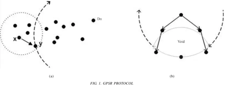
Greedy forwarding works on a simple algorithm, which is to forward packets to neighboring nodes closest to the destination or if the destination is in range then forward it to the destination (very rare case). The source that originates the packet, tags the packet with the destination

information. The decision for the next hop is made on the basis of the destination information, each node is assumed to be aware of its location and the location of the neighboring nodes. To obtain the position of nodes is not an issue considered here. GPS could be used for outdoors and well developed techniques already exist for indoors. Fig. 1(a) shows an example of greedy forwarding where the node x has to forward a packet to the Destination node Dn. Node x selects node y as it is in its radio range (neighboring node) and closest to the destination.

Perimeter forwarding is an alternate technique employed by GPSR to route packets if a void area appears. An example

of a void area is illustrated in Fig. 1(b). Perimeter forwarding is adapted when a node comes across a void area, an area

in which the neighboring node close to the destination is not present. This technique keeps record of the location,

where greedy forwarding fails it tries to figure whether

greedy forwarding could be reintroduced. If greedy forwarding is not an option, it then forwards the packet on

the faces of the planer graph using the right hand rule. There are two faces interior and exterior. While forwarding

data it keeps on checking, whether greedy forwarding is possible or not. If greedy forwarding is possible it switches

to greedy forwarding. This technique keeps forwarding the packet until it reaches the destination, but if a loop

occurs it discards the packet.

FIG. 1. GPSR PROTOCOL

7.

SIMULATION SETUP

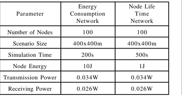
The Simulations were carried out using the NS-2 (Network Simulator-2) [9] and the Mannasim Framework [10]. The simulation parameters used are shown in Table 1. Two separate simulation networks were considered. The Energy consumption network is used to measure the amount of energy consumed by each node in a network using the different location aware routing protocols (SVR, LAR-1, LAR-2, DREAM and GPSR). In the second network, the node lifetime network, the life of the network is investigated, by observing the time at which the first node would die using the different routing protocols.

The major difference in the simulation parameters of the two different networks, the energy consumption network and the node lifetime network, is the node energy and the simulation time, while the remaining parameters are the same. In the node lifetime network the simulation time is increased from 200-500s and the energy is reduced from 10-1J in order to examine the time when the first nodes dies, that is runs out of energy, this trait of the sensor node could not be observed in the energy consumption network.

In the simulation trials two types of node deployments were simulated with each network type, a regular and an irregular scenario. In the first deployment the nodes were regularly uniformly deployed in a flat 400x400m area. Where as in the second network the nodes were randomly deployed in the same area. Although sensor nodes are assumed to be deployed in large numbers, in this simulation 100 nodes were simulated to investigate the routing protocol properties, the number of nodes could be easily increased as the compared routing protocols provide scalability.

8.

RESULTS

The simulations were carried out to investigate the performance of SVR protocol against other location aware routing protocols (LAR-1, LAR-2, DREAM and GPSR). The simulation trials were carried out using the simulation parameters in Table 1.

The results section is further categorized as Node energy depletion and Average energy consumption. In the node energy depletion section, the time the first node dies for both deployments is shown. In the Average energy consumption section, the results present the average energy consumed (based on 30 random iterations) by each node when the simulation time is 200s.

The reliability of routing protocol comes with a trade off, location aware routing protocols provide greater reliability with higher energy consumption. The DREAM protocol has the ability to flood data, which would assure reliable delivery, the LAR protocol could deliver data in a reliable way by increasing the zone sizes and SVR could improve its performance by forwarding a data packet to all its neighbors, which would assure reliability but all these tasks are energy greedy.

8.1

Node Energy Depletion

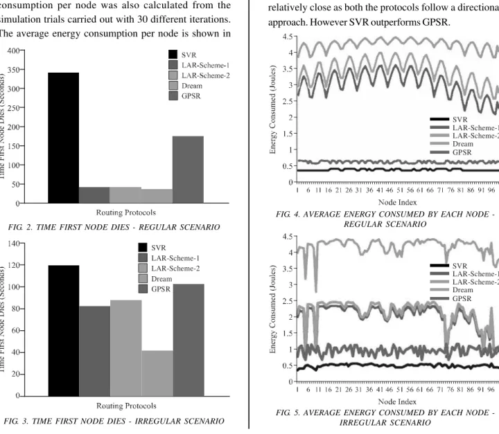
The results shown in Figs. 2-3 show the node energy depletion for a regular and irregular scenario. These results show the time the first node would die using each protocol using the network properties shown in Table 1 with the node lifetime network. While simulating the nodes using the SVR protocol in a regular scenario the first nodes dies at 342 seconds in the simulation. The first node dies under 50 second with the LAR-1, LAR-2 and DREAM routing protocols. The GPSR protocol performs significantly better than LAR-1, LAR-2 and DREAM with the first node depleting it's energy around 176 seconds. Where as for the irregular scenario the SVR protocols performance drops as compared to the regular scenario. The first node dies at around 130 seconds. The performance of 1and LAR-2 protocols in an irregular scenario is better as compared to a regular scenario. The first node dies at around 90 seconds using LAR-1, while using LAR-2 at nearly 100 seconds and with DREAM at around 50 second through the simulation. With the GPSR the first node dies at around 110 seconds.

TABLE 1. SIMULATION PARAMETERS

Energy Node Life

Parameter Consumption Time

Network Network

Number of Nodes 100 100

Scenario Size 400x400m 400x400m

Simulation Time 200s 500s

Node Energy 10J 1J

Transmission Power 0.034W 0.034W

8.2

Average Energy Consumption

The average energy consumption of each node was calculated from the results obtained from the simulation trials with 30 different iterations. The average energy consumption of each node for the regular scenario is shown in Fig. 4 and for the irregular scenario is shown in Fig. 5.

From these results it could be inferred that the performance of SVR and GPSR protocol is better in a regular scenario as compared to the irregular scenario and vice versa for LAR-1 and LAR-2. Where as there is not much change in the performance of the DREAM protocol, it is slightly better in the regular scenario. The average energy consumption per node was also calculated from the simulation trials carried out with 30 different iterations. The average energy consumption per node is shown in

SVR LAR-Scheme-1 LAR-Scheme-2 Dream GPSR

FIG. 2. TIME FIRST NODE DIES - REGULAR SCENARIO

FIG. 3. TIME FIRST NODE DIES - IRREGULAR SCENARIO

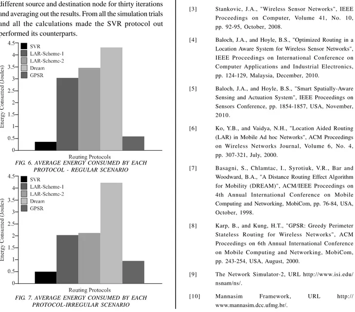
Figs. 6-7 for a regular and an irregular scenario respectively. From the results shown in Figs. 6-7 it could be observed that the SVR tends to consume less energy per average node in the regular scenario than in the irregular scenario and same is the case with the DREAM and GPSR protocol. Where as LAR-1 and LAR-2 consume less energy per average node in an irregular scenario as compared to a regular scenario.

The results obtained from the simulation trials show that the performance of LAR-1 and LAR-2 is close to each other as both the schemes of LAR use a request zone and expected zone. The performance of the dream protocol differs from the rest of the compared protocols as it uses location table. While the performance of SVR and GPSR is relatively close as both the protocols follow a directional approach. However SVR outperforms GPSR.

SVR LAR-Scheme-1 LAR-Scheme-2 Dream GPSR

SVR LAR-Scheme-1 LAR-Scheme-2 Dream GPSR

FIG. 4. AVERAGE ENERGY CONSUMED BY EACH NODE -REGULAR SCENARIO

9.

CONCLUSION

In this paper the role of routing protocol in wireless sensor networks is outlined, followed by an extensive survey on the popular location aware routing protocols. In this paper the SVR protocol is also compared with four other location aware routing protocols LAR-1, LAR-2, DREAM and GPSR.

The energy consumption of each node, the first node depletion time, and the average energy consumed by each node and the average energy consumed per node is also calculated for each protocol. The calculations were made on the basis of two scenarios, a regular and an irregular scenario with different sets of data that is selecting a different source and destination node for thirty iterations and averaging out the results. From all the simulation trials and all the calculations made the SVR protocol out performed its counterparts.

ACKNOWLEDGEMENTS

The authors would like to thank the HEC (Higher Education Commission), Pakistan, for the extended support and Prof. Brian, S. Hoyle, University of Leeds, UK, for his valuable suggestions.

REFERENCES

[1] Akyildiz, I.F., Weilian, S., Sankarasubramaniam, Y., and Cayirci, E., "A Survey on Sensor Networks", IEEE

Proceedings on Communications Magazine, Volume 40, No. 8, pp. 102-114, August, 2002.

[2] Raghavendra, C.S., Sivalingam, K.M., and Znati, T., "Wireless Sensor Networks", Springer USA, 2004.

[3] Stankovic, J.A., "Wireless Sensor Networks", IEEE Proceedings on Computer, Volume 41, No. 10,

pp. 92-95, October, 2008.

[4] Baloch, J.A., and Hoyle, B.S., "Optimized Routing in a Location Aware System for Wireless Sensor Networks", IEEE Proceedings on International Conference on Computer Applications and Industrial Electronics,

pp. 124-129, Malaysia, December, 2010.

[5] Baloch, J.A., and Hoyle, B.S., "Smart Spatially-Aware Sensing and Actuation System", IEEE Proceedings on Sensors Conference, pp. 1854-1857, USA, November,

2010.

[6] Ko, Y.B., and Vaidya, N.H., "Location Aided Routing (LAR) in Mobile Ad hoc Networks", ACM Proceedings on Wireless Networks Journal, Volume 6, No. 4, pp. 307-321, July, 2000.

[7] Basagni, S., Chlamtac, I., Syrotiuk, V.R., Bar and

Woodward, B.A., "A Distance Routing Effect Algorithm for Mobility (DREAM)", ACM/IEEE Proceedings on 4th Annual International Conference on Mobile Computing and Networking, MobiCom, pp. 76-84, USA,

October, 1998.

[8] Karp, B., and Kung, H.T., "GPSR: Greedy Perimeter Stateless Routing for Wireless Networks", ACM Proceedings on 6th Annual International Conference

on Mobile Computing and Networking, MobiCom, pp. 243-254, USA, August, 2000.

[9] The Network Simulator-2, URL http://www.isi.edu/ nsnam/ns/.

[10] Mannasim Framework, URL http://

www.mannasim.dcc.ufmg.br/.

FIG. 6. AVERAGE ENERGY CONSUMED BY EACH PROTOCOL - REGULAR SCENARIO