AUTOMATIC ROAD EXTRACTION FROM SATELLITE IMAGES USING EXTENDED KALMAN FILTERING AND EFFICIENT PARTICLE FILTERING

DOI : 10.5121/ijdps.2011.2613 135

Jenita Subash

Lecturer

Cambridge Institute of technology

K.R.Puram,Bangalore

ABSTRACT

Users of geospatial data in government, military, industry, research, and other sectors have need for accurate display of roads and other terrain information in areas where there are ongoing operations or locations of interest. Hence, road extraction that is significantly more automated than the employment of costly and scarce human resources has become a challenging technical issue for the geospatial community. An automatic road extraction based on Extended Kalman Filtering (EKF) and variable structured multiple model particle filter (VS-MMPF) from satellite images is addressed. EKF traces the median axis of a single road segment while VS-MMPF traces all road branches initializing at the intersection. In case of Local Linearization Particle filter (LLPF), a large number of particles are used and therefore high computational expense is usually required in order to attain certain accuracy and robustness. The basic idea is to reduce the whole sampling space of the multiple model system to the mode subspace by marginalization over the target subspace and choose better importance function for mode state sampling. The core of the system is based on profile matching. During the estimation, new reference profiles were generated and stored in the road template memory for future correlation analysis, thus covering the space of road profiles. .

General Terms

Image Processing, Remote sensing

Keywords

Satellite images, Extended Kalman Filter, Local Linearization Particle filter, Efficient particle filter.

1.

INTRODUCTION

136

initialization system has been proposed based on GIS or geographical database has been reviewed in [1] and [2], and on heuristics [3], [4] or an stochastic assumption [5]. In a semi-automatic method human intervention is required at the initial stage and at times during the processing stage. A notable characteristic of ground target tracking is that prior nonstandard information such as target speed constraints, road networks, and so forth can be exploited in the tracker to reduce the uncertainty of target motion and provide better estimates of the target state[1]. A tracker that ignores or is unable to make use of this additional source of information can only attain limited performance. In the cases of low signal to- noise ratio, the incorporation of such constraint information is essential to successful tracking. Multiple model estimation is widely used in the tracking community to tackle motion uncertainty. The interacting multiple model estimator [7] is one of the best known multiple model estimators. Recent applications of multiple model estimators to ground target tracking were presented in Ref. [6], [8], [9], [10], [11]. Kirubarajan and Bar-Shalom noted that for ground target tracking a multiple model estimator with fixed structure has to consist of a large number of models, owing to the many possible motion modes and various road constraints[8]. It is not only computationally undesirable but also potentially results in highly degraded estimates (due to the excessive “competition” among the many models). In order to overcome this problem, they proposed an adaptive or variable structure interacting multiple model estimator for ground target tracking [8]. The basic idea is that the active model set varies in an adaptive manner and thus only a small number of active models are needed to be maintained at each time. Following the same idea of the variable structure interacting multiple model estimators, a variable structure multiple model particle filters was proposed for ground target tracking [6]. Simulation results showed that the particle filtering based approach has remarkably better error performance. The reasons for the superiority of this particle filtering based approach, as noted in Ref. [12], is that with particles or random samples the simulation-based particle filter is able to incorporate more accurate dynamics models and estimate non-Gaussian distributions (e.g., at an intersection) more accurately than the Kalman filtering-based interacting multiple model estimator. The superiority of multiple model particle filter over the interacting multiple model estimator within the fixed structure multiple model framework was demonstrated in Ref. [12]. Multiple model estimation falls into the category of nonlinear filtering even if every single model is a linear system with Gaussian noise. A sufficient statistic of the hybrid state distribution with a fixed dimension is thus impossible. Moreover, the complexity of the optimal multiple model estimator increases exponentially with time [6]. Both the interacting multiple model estimator and the particle filter are suboptimal nonlinear filtering algorithms that maintain constant complexity and computational expense. The former maintains a constant number (i.e., the number of models) of Kalman filters while the latter maintains constant number of (the most likely) particle trajectories. Such sub-optimality is inevitable for practical purposes.

137

proposes a method based on the combination of EKF and VS-MMPF. The EKF component is responsible for tracing axis coordinates of a road until it encounters an obstacle or an intersection. VS-MMPF is responsible for tracing road branches on the other side of a road junction or obstacles.

A method of feed forward neural network applied on a running window to decide whether it

contains a three- or a four arm road junction has been reviewed in [16].This method suffers from quite many false alarms. But PF algorithm can find road junctions and track each of the road branches one after the other. Extracted of road from one raster image need not be extracted in the same way from another raster image, as there can be a drastic change in the value of important parameters based on nature’s state, instrument variation, and photographic orientation has been reviewed in [7]. Parameters used for extraction are its shape (geometric property) and gray-level intensity (radiometric property).No contextual information was used. The method works solely on image characteristics. The method is semi-automatic, with manual selection of the start and end of road segments in the input image.

2.

AUTOMATIC ROAD EXTRACTION

The road tracking process starts with an automatic seeding input of a road segment, which

indicates the road centerline. From this input, the computer learns relevant road information, such as starting location, direction, width, reference profile, and step size. This information is then used to set the initial state model and the related parameters are estimated the road is tracked automatically by EKF and VS-MMPF.

2.1 Application Background

In a road tracking procedure, when the system recognizes tracking failure, it returns the control to the human expert and uses the guidance of the human operator to update its set of profile predictors and continue tracking the road afterward. This approach is robust in extracting a single road track due to its interface with human experts, but it cannot identify and handle multiple road branches when it encounters an intersection of several roads. Information about road intersections or junctions is of high importance in understanding road network topologies. In [9], junction hints are used in the network optimization process by forcing roads to pass through detected T- and L-shaped junctions. For example, [16], [17] and [18] used a feed forward neural network applied on a running window to decide whether it contains a three- or a four-arm road junction. This method suffers from quite many false alarms. In [19], [20] a method is developed for intersection detection based on pixel footprints. This algorithm finds the footprint of a pixel as the local homogenous region around the pixel enclosed by a polygon, and then, by identifying the toes of a footprint, it can track a road path, thus identifying the road intersections. But when this algorithm encounters a road width obstacle, it might lose track of the road.

2.2

Normal or Body Text

138

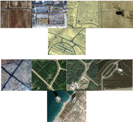
observation mission -1), Kompsat EOC and KVR-1000 satellite. A number of the more frequently used sensors is IKONOS. IKONOS is a satellite image which is launched in September 1999. The device features a panchromatic and multispectral sensors that captures data at a resolution of 1m and 4 m respectively. The multispectral sensor captures the RGB bands as well as Near Infrared(Nir) band. A

139 Fig 2: Pie chart representation of satellite images using different sensors

pan-sharpened version of the data is available, where the panchromatic and multispectral data is combined to produce. Sample of satellite images is shown in Fig 1. and the researches of different satellite imagery in chart form is shown in Fig 2.

3.

SYSTEM OVERVIEW

A number of semi-automated RNE approaches require a human operator to specify the seed points before a higher level operation can continue with the extraction process, Automating the seeding process reduces the total extraction time of such a system significantly. According to Harvey [16], the performance of automatic road tracking algorithm depends to a large extend on the quality of starting points. Apart from automating process the quality of the seed points is consequently also imperative.

Satellite Image

Canny edge detection

Extended kalman Filter

Efficient Particle Filter Road Junction

Dead end

Initializing road branches Profile matching

140 Fig 3: Workflow of road extraction method

3.1

Automatic seeding

The workflow of the road extraction method is as shown in Fig 3. In the content of road extraction, seeding is the process whereby a marker is placed at certain points of interest within a road network. These points of interest can include markers along the centre of the road, point of high curvature, or intersections. The seeds are typically single points but can also be centerline segments or road regions. Seeding is not an extraction technique itself, but the marker are used as initialization points for extraction technique, such as road tracker and snakes. The seeds can also be used to generate road models (pattern classes), which can be used to train classifiers used to detect road objects in imagery, In addition, road network construction algorithm can also use seeds to connect the points using a high-level algorithm. A wide variety of techniques can be employed to detect road seeds automatically. Some of the technique includes parallel edge detection, geometric template matching, segmentation, Haugh transform and spectral classification. Automatic seeding algorithms can be categorized as low to medium level processing technique, as they typically receive raw image data or output from a low level algorithm as input. One of the most popular approaches to automatic seeding is the detection of parallel edge in medium to high resolution imagery.

3.2

Canny edge detection

141 3.3 Profile matching

A gray-level profile, extracted perpendicular to the road direction, is a very characteristic property on a road. It often shows a good contrast between the road surface and its vicinity. Thus, like in [2], we also utilized the method of gray-level profile matching to acquire observations needed in the tracking algorithm. The method in [2] uses the least square error profile matching to measure the similarities between any two profiles and also to estimate the optimum shift that exists between them. In our approach, the correlation coefficient and the difference between the profile means are used to calculate the error or difference between any two profiles. This error is calculated as follows:

2

1 2 2 1 2

2 2 2 2 1 1

2 2 1 1 1

2 1 2 1

p

)

p

p

(

e

)

p

(p

)

p

(p

)

p

)(p

p

(p

1

e

2

e

e

}

p

,

Error{p

−

=

−

−

−

−

−

=

+

=

Error where p1 and p2 are two gray-level profiles. The first term e1 describes the dissimilarity between the shapes of the two gray level profiles, and the second term e2 measured the difference between the average intensity values of the two road profiles. The profile clustering algorithm is described in Algorithm 1.

Algorithm 1. Update profile clusters

Let p denote the new road profile at the kth step and ci, for i = 1, 2, . . . , C, denote the ith cluster if there are any young clusters that must be verified, then determine whether the young clusters must be authorized or rejected

end if

for j = 1 to C, do

di distance between p and cj end for

dmin min{d1, d2, . . . , dC} if dmin threshold, then

update the present clusters if necessary

else if p passes the validation tests, then

produce a new young cluster by p cC+1,

142 end if

3.4

Extended Kalman Filtering

The state vector contain the variable of interest. It describes the state of the dynamic system and represents its degree of freedom. The variable in the state vector cannot be measured directly but they can be inferred from values that measurable. In case of road tracking from an image, it

includes where rk and ckare the coordinates of road axis points, k is the direction of the road,

k and is the change in road direction. The distance along the road is considered to be as time

variable. To illustrate the principle behind the EKF, consider the following example. Let W be a random vector and

y = g (x) (1)

be a nonlinear function, g : Rn → Rm. The question is how to compute the pdf of y given the pdf

of xi For example, in the case of being Gaussian, how to calculate the mean (y) and covariance

( y) of y> If g is a linear function and the pdf of x is a Gaussian distribution, then Kalman filter

(KF) is optimal in propagating the pdf. Even if the pdf is not Gaussian, the KF is optimal up to the first two moments in the class of linear estimators [14]. The KF is extended to the class of nonlinear systems termed EKF, by using linearization. In the case of a nonlinear function (g(x)), the nonlinear function is linearized around the current value of x, and the KF theory is applied to

get the mean and covariance of y. In other words, the mean

(

)

(

)

y

P of y,

given the mean (x) and covariance (Px) of the pdf of x are calculated as follows:

Road axis points are tracked using recursive estimation, and the state model is given by

[

]

k k k

k

r

c

x

=

where rt and ctare the coordinates of road axis points, t is the direction of the road, t and is the change in road

direction.

(

)

y = g(x) (2)

(

)

y

P = (∇g)P_x(∇g)T, (3)

where (

∇

x

Algorithm 2. Extended kalman filter

143 xk = f (xk−1, vk−1, uk−1) (4)

yk = h (xk, nk, uk) (5)

k

w

dk

dk)

(

cos

dk

c

dk)

(

sin

dk

r

x

+

+

+

⋅

+

+

⋅

−

=

k

x

v

0

1

0

0

0

0

1

0

0

0

0

1

Z

=

+

where x ∈

_R

is noise, v ∈

_R

n∈

_R

the observation noise, u the point and the noisy observation of the system. The nonlinear functions f and h are need not necessarily be continuous. The EKF algorithm for this system is presented below:

• Initialization at k = 0: ], x [ E xˆ0= 0

], ) xˆ x ( ) xˆ x [( E

P_{x 0 0 0 0} T

0 = − −

], ) v v ( ) v v [( E

P_v = − − T

], ) n n ( ) n n [( E

P_n = − − T

For k = 1, 2, . . . . ∝. (1) Prediction step.

(a) Compute the process model Jacobians:

, | ) u , v , x ( f F 1 k

k x k 1 x xˆ

x =∇ − = −

Gv=∇vf(xˆk−1,v,uk)|v=v

(b) Compute predicted state mean and covariance (time update)

), u , v , xˆ ( f

xˆ_{k k}−_{1 k}

− = . G P G F P F

P_xk− = _{xk xk xk}T + _{v v} T_v

(2) Correction step.

144 , | ) u , n , x ( h H k

k x k x xˆ

x − = ∇ = n n k k n

n h(xˆ ,n,u )|

D = − ∇ = − − − − = 1 0 0 0 dk 1 0 0 sin(u) dk 0.5 (u) sin d 1 0 (u) cos dk 0.5 cos(u) dk 0 1 Fˆ 2 2 k k

(b) Update estimates with latest observation (measurement update)

1 T n n n T xk xk xk T xk xk

k P H (H P H D PD )

K = − − + − xˆ_k =xˆ−_k+K_k[y_k−h

(

)

−

−

= _{k xk xk}

xk (I K H )P

P

Qk =

0.01 0 0 0 0 0.02 0 0 0 0 0.04W 0 0 0 0 0.04W

Rk =

1 0 0 0 0.4W 0 0 0 0.4W 2 θ σ

3.5

Particle Filtering

Multiple dynamics models are used to account for the motion uncertainty due to target maneuver. We assume the motion mode state r = 1 corresponds to the cruise mode, r = 2 corresponds to the maneuver mode, and r = 3 corresponds to the stopped mode. According to the idea of variable-structure multiple-model approach, the cruise and the maneuver modes are active all the time, whereas the stopped

mode is active only when there is no detection. The stopped

mode is added to the active mode set when the target is no longer detected and removed after the target is detected again. The target dynamics models for different target modes have the same linear Gaussian structure, given by Eqs. (3) and (8). For the maneuver model, large process noise along the road is used, which is of the order of the magnitude of the maximum acceleration. Much smaller process noise is used in the cruise model. In the stopped model, the process noise is set to zero. The target velocity in the stopped target model is also set to zero. The road

information in terms of the reference point _Po

145

incorporated in the dynamics models through xOk , and G. The transition of the motion mode r is assumed to occur only at sensor sampling instants and is governed by the transition probability matrix P, whose elements are defined by

p

=

p(r

=

j

r

=

i)

where pij satisfy s₌

=

1

j

p

1

columns of the matrix P). For sake of simplicity, constant P is used. The active mode set may be {1, 2} or {1, 2, 3}. Hence, four transition matrices in total are needed. The initial guess of the transition matrices are calculated based on the sojourn time of the modes[4]. Because the knowledge of the present road segment is required for the propagation of the dynamics models, a

pointer pk pointing to the road segment the target is on at time tk is used as an auxiliary mode

state. All the information about the present road segment, such as its endpoints, directions, and

neighbors, is indexed in the road database via the pointer pk. The update of pk is determined by

the propagated target position. The sequence pk is not a Markov chain because of its target state

dependence. If after propagation the target remains on the present road segment, pk does not

change its value; if the target leaves the present road segment to enter a new segment, pk points

to the new segment, too. When there is only one new segment to enter, the pointer is updated without ambiguity. However at an intersection where more than one road meets, it is uncertain which road segment the target would enter. Then all the hypotheses have to be considered and

thus pk and xk in the particle filter have to be updated in a probabilistic manner. The ambiguity

can only be eliminated after new observations are available. If no prior knowledge about the route or destination of the target is available, then it is reasonable to assign identical probability to each hypothesis.

Suppose the number of roads to enter is L, the probability to

enter any road segment is 1/L. A single observation model of a detected target is used, as given by Eq. (11). In other words,

p(yk|xk, rk = 1) = p(yk|xk, rk = 2).

When the target is detected, the likelihood of a moving mode can be computed using yk and the

system model; the likelihood of the stopped mode is zero. (The probability of detection PD may be incorporated in the likelihood of the moving mode, but it is not necessary since PD is a common factor among the stopped and moving modes.)

Do not include headers, footers or page numbers in your submission. These will be added when the publications are assembled.

4.

EFFICIENT PARTICLE FILTERING

146

Hence, the conditional distribution p(x R ,Yk)

(i) k

k is not strictly Gaussian. It is, however, still

approximated by a Gaussian distribution whose mean ˆ(i)

k

x and covariance P_k(i) are an

approximate sufficient statistic and are updated using unscented Kalman filtering. The details of the unscented Kalman filter can be found in Ref. [12]. For nonlinear filtering problems, when the parameters of the unscented transformation are appropriated tuned, the unscented Kalman filter can yield better estimation results than the extended Kalman filter. The likelihood

)

,

ˆ

,

(

)

,

,

(

k k

i k k

k

r

R

Y

p

y

r

x

P

y

p

≈

used for recursive sampling of rk is also calculated based on Gaussian approximation. That is,

{r_k(i),xˆ(i)_k ,P_k(i),p(i)_k ,w(i)_k}_iN₌₁

Given rk(i) , ) (

ˆi k

x , Pk(i)and , the mean and covariance P(i)yk of yk are estimated using standard

unscented transformation. The full particle representation is given by

i=1, where ˆx(i)k and P(i)k are deterministically updated given r(i)k and p(i)k . The outline of a filter cycle of the efficient particle filter for road-constrained target tracking is given in Table II.

Algorithm 3. Efficient Particle filter

For i = 1, . . . , N,

- determine the active motion mode set for ith _{particle at t} k

- determine the transition probability matrix P_k(i)

- For j = 1, . . ., S, where S is the number of active motion modes (hypothesis)

o propagate xˆ(_ki₋)₁ and P_k(₋i)₁ through the model specified by mode j and road segment P_k(i₋)₁ to generate xˆ*(_ki,j,l) and )

l , j , i *( k

P , where l = 1, . . . , L(i,j) _{(if the target does not cross an intersection, L}(i, j) _{= 1; if the target crosses an intersection, L}(i, j) _>

1; if the target crosses an intersection, L(i, j) _{> 1; determine} *(i,j,l) k

P according to xˆ*(_ki,j,l) and P_k*(i,j,l)

- For j = 1, . . ., S and for l = 1, . . ., L(i, j)_{, evaluate the likelihood} (i,j,l) ₁

k

=

Λ

o if the target is not detected if j = 3,

Λ

=

if j = 1 or 2 AND the target is hidden or moves perpendicular to the line of sight,

Λ

=

if j = 1 or 2 AND the target is in normal motion,

Λ

=

o if j = 3 OR the target is hidden or moves perpendicular to the line of sight,

Λ

=

147 ) j , i ( L 1 l S 1 j ) i ( 1 k ) i ( k w w = =

−

Σ

Σ

∞

Λ

=

- Resampling :

Multiple / Discard

{

}

1 i ) l , j , i ( k ) l , j , i ( * k ) l , j , i ( * k ) l , j , i ( * k ) i ( 1

k ,xˆ ,P ,p ,

r₋ Λ ₌ to high / low importance weights w(_ki) to obtain N new

{

}

1 i ) l , j , i ( k ) l , j , i ( * k ) l , j , i ( * k ) l , j , i ( * k ) i ( 1

k ,xˆ ,P ,p ,

r− Λ ₌ with equal wieghts.

For i = 1, . . . , N, sample

) j , i ( ) i ( 1 k k ) l , r , i *( k ) l , r , i *( k k ) i ( ) i (

k ,l )~pˆ(y |xˆ ,P )p(r |r )/L

r

( k k

− where pˆ(y |xˆ ,P ) ;set

) l , j , i ( k ) l , j , i *( k ) l , j , i *( k

k =Λ

) l , r , i *( ) i ( k l , r , i *( k ) i ( k l , r , i *( k ) i ( k ) i ( ) i ( k ) i ( ) i ( k ) i ( ) i (

k

_,

_P

_P

_,

_p

_p

xˆ

xˆ

=

=

=

For i = 1, . . ., N update xˆ_k(i),P_k(i) from P_k−(i) based on

Gaussian approximation and update p(_ki)according to xˆ(_ki) and P_k*(i,j,l)

5.

RESULTS AND DISCUSSION

Road extraction from remote sensing images has its applications in cartography, urban planning, traffic management and in industrial development. In order to evaluate the results, we compare the obtained road lane feature to a manually digitized reference road dataset. Figure.4 shows the road tracking results in IRS image. First the reference profile and seed point is extracted automatically by automatic seeding technique. Then the edge of the road is detected using Canny edge detection. Then the road network is tracked by EKF until it reaches a road junction or obstacles. Then the role is given to the efficient particle filter to initialize the seed point of the road branch. For larger dk, progress of the EKF and Efficient particle filter modules will be faster on the image; however, the resolution of the resulting road center points will be coarser.

The system error covariance matrix Qk is a measure of how our road model matches the road

behavior. If the roads in the image are changing direction rapidly, we have to set high values for

the elements of Qk. The measurement error covariance matrix Rk models the behavior of the

error resulted from our measurements from the image. Fig 4. Shows the results of automatic road extraction using EKF and EPF.

148 (c) (d)

(e) (f)

(a) (b)

149 (e) (f)

(a) (b)

(c) (d)

Fig.4: Automatic road tracking results from an IRS image using Efficient particle filtering (a) Satellite image (b) Monochromatic imagery (c) Automatic seeding (d) Edge detection using Canny edge detection (e) Road tracking by EKF (f) Road tracking by Efficient particle filtering and EKF.

150

values are very high, about 0.89 and completeness is about 0.83. The completeness of the result depends on the complexity and properties of the road network. The root mean square error value is calculated for EKF using

(

)

− =

m

1 i

2 i k K

xˆ

x

k = 1,2,...,10 ; m = 100

where

xˆ

obvious that the target is tracked for 100 data samples. The RMSE value while using EKF is comparably very low when compared to EPF, and is shown. Fig.5 shows the change in row, column and direction of the road in automatic road extraction technique.Fig 6. Shows the road extraction using profile matching.

151 Fig 5: Road extraction using profile matching

6.

CONCLUSION

For road-constrained targets, the incorporation of road information into the dynamics models can greatly reduce the target motion uncertainty. Unscented Transform has been used in the kalman filter frame work and the resulting filter is said to be as Unscented Kalman Filter. Using UKF instead of EKF in the VS-MMPF improves the performance. In addition to this a set of training data sequence can be used to automatically optimize the parameters of a particle filter. A variable-structure, multiple-model framework is used to address target maneuvers along the road. The proposed efficient particle filter is approximations to the optimal particle filter for jump Markov linear Gaussian systems. The main approximation of the filter is the Gaussian assumption about the conditional target state distribution given a mode sequence and observations. The efficient particle filter with 80 particles yields satisfactory simulation results.

7.

ACKNOWLEDGMENT

We gratefully acknowledge the support by Cambridge Institute of technology,Bangalore.

8.

REFERENCES

[1] A.Baumgartner,C.T.Steger,C.Wiedemann,H.Mayer,W.Eckstein,H.Ebner,”Update of roads in GIS from aerial imagery:Verification and multi-resolution extraction,”in Proc.Int.Archives of Photogrammetry and remote sensing,1996,vol.XXXI B3/III,pp.53-58

[2] Dan Klang,”Automatic detection of changes in road database using satellite imagery,”in Proc.Int.Archives of Photogrammetry and remote sensing,1998,vol.32,pp.293-298

[3] C.Steger,”Extracting curvilinear structures :a differential geometric approach,”in Proc.of Europeans Conference on Computer Vision,1996,pp.630-641

152

[5] M.Barzohar and D.B.Cooper,”Automatic finding of main roads in aerial images by using goometric-stochastic models and estimation,”IEEE Trans.on Pattern Analysis and Machine Intelligence,vo.l.8,no.7,1996,pp.707-721

[6] B. Ristic, S. Arulampalam, and N. Gordon, Beyond the Kalman Filter:Particle Filters for Tracking Applications. Boston, MA: Artech HousePublishers, 2004.

[7] Y. Bar-Shalom, X. R. Li, and T. Kirubarajan, Estimation with Applications to Tracking and Navigation: Theory, Algorithms and Software.New York, NY: John Wiley and Sons, Inc., 2001.

[8] T. Kirubarajan, Y. Bar-Shalom, K. R. Pattipati, and I. Kadar, “Ground target tracking with variable structure imm estimator,” IEEE Transactions on Aerospace and Electronic Systems, vol. 36, no. 1, pp. 26 – 46, January 2000.

[9] T. Kirubarajan and Y. Bar-Shalom, “Tracking evasive move-stop-move targets with a gmti radar using a vs-imm estimator,” IEEE Transactions on Aerospace and Electronic Systems, vol. 39, no. 4, pp. 1452 – 1457,October 2003.

[10] C. Kreucher and K. Kastella, “Multiple model nonlinear filtering for low singal ground target applications,” in Proceedings of SPIE Conference on Aerosense, Signal Processing, Sensor Fusion and Target Recognition X, vol. 4380, April 2001, pp. 256–266.

[11] L. Lin, Y. Bar-Shalom, and T. Kirubarajan, “New assignment-based data association for tracking move-stop-move targets,” IEEE Transactions onAerospace and Electronic Systems, vol. 40, no. 2, pp. 714 – 725, April 2004.

[12] A. Doucet, N. de Freitas, and N. Gordon, Sequential Monte Carlo Methods in Practice. New York, NY: Springer-Verlag, 2001.

[13] J.Mena, “State of the art on automatic road extraction for GIupdate: A novel classification,” Pattern Recognit. Lett., vol. 24, no. 16,pp. 3037–3058, Dec. 2003.

[14] Mckeown,D.Denlinger,J.L.,”Cooperative methods for road tracking in aerial imagery”,In:Workshop Comput.Vision Pattern Recognition,pp.662-673,1988.

[15] G. Vosselman and J. D. Knecht, “Road tracing by profile matching and Kalman filtering,” in Proc. Workshop Autom. Extraction Man-Made Objects Aerial Space Images, Birkhaeuser, Germany, 1995, pp. 265–274.

[16] M. Bicego, S. Dalfini, G. Vernazza, and V. Murino, “Automatic roadextraction from aerial images by probabilistic contour tracking,” in Proc.ICIP, 2003, pp. 585–588.

[17] A. Barsi and C. Heipke, “Artificial neural networks for the detectionof road junctions in aerial images,” ISPRS Arch., vol. 34, pt. 3/W8,pp. 113–118, Sep. 2000.

[18] J.Zhou,W.F.Bischof and T.Caelli,”Road tracking in aerial images based on human computer interaction and Bayesian filtering,”ISPRS J.Photogram.Remote sens.,vol.61,no.2,pp.108-124,2006

[19] C. Wiedemman, C. Heipke, H. Mayer, and O. Jamet, “Empirical evaluation of automatically extracted road axes,” in Empirical Evaluation Techniques in Computer Vision. Piscataway, NJ: IEEE Press, 1998,pp. 172–187.