HIV Infection in T-lymphocytes and Drug Induced CTL
Response of a Time Delayed Model
Priti Kumar Roy
∗†Amar Nath Chatterjee
‡Biplab Chattopadhyay
§Abstract—Drug therapy response of HIV-1 infected immune system is an important area of research by now. Today, a greater knowledge of drug induced CTL response allows us to better understand of cell mediated immune mechanism and humoral immune mechanism for viral infections. Moreover excessive stimulation of CTL in the immune system by different drugs leads to protective effects during natural infec-tion with Human immunodeficiency virus of type-1. This paper concerns an application of drug therapy response to a mathematical model related to HIV-1 infection dynamics including a time delay in the re-moval of infected CD4+T cells or analogously in the process of viral replication. The model is analysed analytically as well as numerically. Our results show that delay affects considerably the attainability of the reduction of viral load in the HIV-1 infected system.
Keywords—Asymptotic Stability, CD4+
T cells, Cell Lysis, CTL, Immunodeficiency Virus of type-1, RTI, Time Delay, Time Series Solutions.
1
Introduction
Extensive research on the area of HIV-1 infection invad-ing the human immune system started in early nineties of the last century [1]-[3]. Though considerable knowledge have been gathered till date regarding the implications of genetic variation of immune cells, HIV-1 pathogenesis and probable therapies treating the infected individuals, many of the issues still remain unsolved. Recent effort in this direction relates to the retroviral therapies used to treat HIV-1 patients making them to survive for a longer period against the odds of probable opportunistic diseases. Actually retroviral therapy when given to an individual patient make a portion of the immune cells to be toxic thereby introducing toxicity in the immune
sys-∗Research is supported by the Department of Science and
Tech-nology, Government of India, Mathematical Science office, No. SR/S4/MS: 558/08 and its a pleasure to acknowledge All India Council for Technical Eduction for their travel support to present the research work in WCE 2010, U.K.
†Centre for Mathematical Biology and Ecology, Department of
Mathematics, Jadavpur University, Kolkata 700032, West Bengal, India. Corresponding Author E-mail: [email protected], Fax No. +913324146584, Ph.No. +919432095603.
‡Dum Dum Prachya Bani Mandir for Boys’ (H.S), 4 Sath Bagan
Road, Kolkata-700020.
§Department of Physics, Barasat Government College, 10 K. N.
C. Road, Barasat, Kolkata 700124, West Bengal, India
tem of the individual. It is thus important to maintain an optimum controlled level of drug injection for an indi-vidual patient. This very issue of optimal drug therapy together with the dynamical evolution of CD4+T
lym-phocytic immune cells needs proper understanding. In this communications we make an attempt to understand bearings of drug response on the dynamical behaviour of the lymphocytic immune cells populations specifically CD4+T cells together with that of viral load.
It has been observed clinically that patients infected with immunodeficiency virus type-1 (HIV-1), if treated with a combination of inhibitor-drugs lamivudine and zidovu-dine shows a 10 to 100 fold reduction of viral load and nearly 25% increase in the healthy CD4+T cells count.
Sustenance of such drug receiving patients is observed to be more than one year [4], [5]. The longer sustenance is admitted to be consequences of the diminishing rate of infections of the uninfected T-cells. Obviously leads to the conjecture that the drug effectively drives the virus to state of near extinction.
In this paper we consider a mathematical model of HIV-1 infection to CD4+T cells including the
mentioned inhibitor drug. The system response to the drug-stimulation by generating Cytotoxic T-Lymphocyte(CTL) and this CTL’s in-turn attack the ac-tively infected CD4+T cells and kill them. Note that
there exists a finite time lag between a CD4+T cells
get-ting actively infected and its subsequent death. Such re-alistic time lag has been incorporated in the model under consideration. We analyze the dynamics of such a model to understand how the HIV-1-infected immune system responds to varied levels of drugs applied under the sys-tematic therapy procedure.
Formulation of the mathematical model
Let x(t) and y(t) be the uninfected and infected (virus producing cells) portions of the hosts CD4+T immune
cells at a time t. Our focus here is to construct first a simple model for viral dynamics. For this purpose the following assumptions are made.
(A1): Infectible CD4+T cells are produced at a constant
drug induced changes at the steady state the variable cor-responding to free virus can be omitted. At the steady state it is inherently assumed that the free virus popula-tions is proportional to the virus-producing CD4+T cells
which are already infected. Note that infected CD4+T
cells produce free virus by their replication through the process of cell lysis.
(A2): The process of infection to the infectible CD4+T cells follows the law of mass action under mixing homo-geneity. This means that the number of new infection at the steady state is proportional tox(t)y(t).
(A3): A per capita death rate of infected CD4+T cells is
considered and is denoted by a parameter a.
Based on the above assumption we can write down a sim-ple model for virus dynamics as
dx
dt =λ−dx−βxy dy
dt =βxy−ay
(1.1)
whereβis the rate of contact between uninfected CD4+T
cells with the virus producing T- cells. Although it can be seen in the literature that the rate at which unin-fected CD4+T cells are converted into virus producing
(infected) portion is smaller thanβ, we consider here the rate to be same asβ. The argument in support of such enforcement goes as-at steady state the condition of mix-ing homogeneity is well set and the law of mass action holds perfectly. Whenever a HIV-1 infected patient is subjected to RTI (Reverse Transcriptase Inhibitors) drug, the virus replications within the virus producing T-cells faces a reduction. Such effect may be incorporated in the two variable simple virus dynamics model by reducing the numerical value of the parameter β (rate of infec-tion). However, mere reduction of β in the basic viral dynamics model fails to explain the strong suppression of equilibrium virus load observed during long term drug therapy. Therefore it is imperative to include another variable in the basic viral dynamics model (1.1), in order to make the long term immune response of the model at per with those observed in reality. We include a variablez
to represent the density of the Cytotoxic-T-Lymphocyte (CTL) responses against virus infected cells. The basic virus dynamics model with this inclusion becomes
dx
dt =λ−dx−βxy dy
dt =βxy−ay−pyz dz
dt =ky−bz
(1.2)
Here pis the killing rate of the virus producing cells by CTL, k is the rate of stimulation (production) of CTL and b denotes the base line mortality rate of CTL. The basic viral dynamics model including CTL response as-sumes an instantaneous death of infected CD4+T cells.
But in reality the infected T-cells are observed to have a latency period. During this latency period replication or reproduction of virus takes place within the infected cells. Thus, we consider a delay in the death term of infected (virus producing) T-cells. The average effect of such
de-Figure 1: Time series solutions of model variables for different values of delay factor τ. p= 0.001 changes in the time series solutions with the increase of τ. Various model parameters are as in Table 1.
lay can be incorporate through a memory function or de-lay kernel, which under suitable conditions, yields model equations including a delay factorτ (≥0) as
dx
dt =λ−dx−βxy dy
dt =βxy−ay(t−τ)−pyz dz
dt =ky−bz
(1.3)
under the initial condition: x(θ)≥0,y(θ)≥0,z(θ)≥0,
θ∈(−∞,0]
2
Local stability analysis
Right hand side of the equation (1.3) is a smooth func-tion of x, y, z (variables) and the parameter, as long as the quantities are non-negative, so local existence and uniqueness properties holds in the positive octant. The modal equation (1.3) has the following equilibria on all the co-ordinate planes,E0(0,0,0),E1(λd,0,0), and E∗
(x∗ , y∗
, z∗
)
where x∗
=(abβ−dkp)+
√
(abβ−dkp)2+4β2bpkλ 2bβ2
y∗
=λ−dx∗
βx∗ , z
∗
= k(λ−dx∗)
βbx∗
E∗
exists providedk < abβpd, x∗ <λd.
Here we are interested to investigate the local stability of the interior equilibrium E∗
of the delay-induced sys-tem (1.3). Letm(t) =x(t)−x∗
, n(t) =y(t)−y∗
, q(t) =
z(t)−z∗
are the perturbed variables. The linearized form of the system (1.3) atE∗
(x∗ , y∗
, z∗
) is given by
dm
dt =−dm−βmy
∗
−βnx∗
dn
dt =βmy
∗
+βnx∗
−an(t−τ)−pnz∗
−pqy∗
dq
dt =kn−bq
(2.1)
The characteristic equation of system (2.1) is given by
ρ3+(A+ae−ρτ
)ρ2+(B+Ce−ρτ
)ρ+D+Ee−ρτ
= 0 (2.2)
where, A = b+d+βy∗
+pz∗
−βx∗
, B = bd+
dpz∗
+βby∗
+βpy∗ z∗
+bpz∗
+pky∗
−βdx∗
−βbx∗
, C=
a(d+b+βy∗
), D=dbpz∗
+dpky∗
+βbpy∗ z∗
+βpky∗2
−
βdbx∗
Now to determine the nature of the stability, we require the sign of the real parts of the roots of the system (2.2).
Let Φ(ρ, τ) =ρ3+ (A+ae−ρτ
)ρ2+ (B+Ce−ρτ
)ρ
+D+Ee−ρτ
= 0
(2.3) Forτ= 0, i.e. for non-delayed system
Φ(ρ,0) =ρ3+ (A+a)ρ2+ (B+C)ρ+D+E = 0 From Routh-Hurwitz condition, the necessary and sufficient condition for locally asymptotic stability of the steady state is, (A+a)(B +C)−(D +E) > 0 and the non-delayed system is locally asymptotically stable around the positive interior equilibrium if
y∗ > x∗
, and θ >max(θ1, θ2, θ3, θ4)
θ1=βx
∗
z∗ , θ2=
β2
x∗y∗
dz∗ , θ3=
βd2
x∗
abz∗ , θ4=
β2
bx∗y∗
adz∗
(2.4)
Substitutingρ=u(τ) +iv(τ) in (2.2) and separating real and imaginary parts we obtain the following transcenden-tal equations:
u3−3uv2+A(u2−v2) +a(u2−v2)e−uτ
cosvτ
+2auve−uτ
sinvτ+Bu+Cue−uτ
cosvτ
+Cve−uτ
sinvτ+D+Ee−uτ
cosvτ = 0
(2.5) 3u2v−v3+ 2Auv+ 2auve−uτ
cosvτ−
a(u2−v2)e−uτ
sinvτ +Bv+Cve−uτ
cosvτ
−Cue−uτ
sinvτ−Ee−uτ
sinvτ = 0
(2.6)
3
Sufficient Conditions for Nonexistence
of Delay Induced Instability
To find the conditions for nonexistence of delay induced instability, we now use the following theorem of Gopal-samy [6].
Theorem 3.1: A set of necessary and sufficient
condi-tions for the equilibriumE∗
to be asymptotically stable for all τ ≥ 0 is the following: (i) The real parts of all the roots of φ(ρ,0) = 0 are negative. (ii) For real v and
τ ≥0,φ(iv, τ)6= 0, wherei=√−1.
Proof: Here φ(ρ,0) = 0 has roots whose real parts are negative provided (2.4) holds. Now forv= 0
φ(0, τ) =dbpz∗
+dpky∗
+βbpy∗ z∗
+βpk(y∗
)2−βdbx∗
−ab(d+βy∗
)6= 0
(3.1) and forv6= 0
φ(iv, τ) =−iv3−Av2−av2e−ivτ
+iBv+iCve−ivτ
+D+Ee−ivτ
= 0
(3.2) Separating real and imaginary parts we get
Av2−D=Cvsinvτ + (E−av2) cosvτ (3.3)
−v3+Bv= (E−av2) sinvτ−Cvcosvτ (3.4)
Squaring and adding the above two equation, we get
(Av2−D)2+ (−v3+Bv)2=a2v4
+ (C2−2aE)v2+E2 (3.5)
Let the right hand side of (3.5) be denoted byf(v). Now for arbitrary realv , we get from (3.5)
f(v)≤a2v4+ (C2−2aE)v2+E2 (3.6)
Therefore a sufficient condition for the non existence of a real numbervsatisfyingφ(iv, τ) = 0 can now be obtained from (3.5) and (3.6) as
v6+ (A2−2B−a2)v4+ (B2−2AD−C2+ 2aE)v2
+D2−E2≥0 The inequality we can write in the form of
v6+P v4+Qv2+R >0 (3.7)
P =A2−2B−a2, Q=B2+ 2aE−2AD−C2, R=D2−E2.
The sufficient condition can be obtained as if
p > 2βxz∗∗, a
−1 > b−1
+d−1
, and pk >bdxy∗2∗ (3.8)
Therefore condition (i) and (ii) of the above theorems are satisfied if (3.5) holds.
4
Estimation of the length of Delay to
Preserve Stability
In this section we assume that in absence of delay,E∗
is locally asymptotically stable. This is guaranteed if (2.4) holds. By continuity and for sufficiently small τ > 0, all eigenvalues of (2.3) have negative real parts provided one can guarantee that no eigenvalue with positive real part bifurcates from infinity (which could happen since it is a retarded system). For stability analysis we use the Nyquist criterion [7]. To do this, we consider the system (2.1) and the space of real valued continuous functions defined on [τ,∞) satisfying the initial conditions. Let ¯m(L), n¯(L), and ¯q(L) be the Laplace transform of
m(t), n(t), and q(t) respectively. Taking the Laplace transformation of system (2.1), we have
(L−A1) ¯m(L) =A2¯n(L) +m(0)
(L−B2−B3e−Lτ)¯n(L) =B1m¯(L) +B4q¯(L)+ B3e−LτK1(L) +n(0)
(L−C2)¯q(L) =C1¯n(L) +q(0)
(4.1)
where
K1(L) =
Z 0
−τ e−Lδ
n(δ)dδ
K2(L) =
Z 0
−τ e−Lδ
V(δ)dδ; t−τ=δ
A1=−δ1=−(d+βy∗) A2=−δ2=−βx∗ B1=δ3=βy∗ B2=δ4=βx∗−pz∗
B3=−δ5=−a B4=−δ6=−py∗ C1=k C2=−δ7=−b
Rearranging we get
[L3+ (δ1+δ7−δ4+δ5e−Lτ)L2+ (δ2δ3−δ1δ4+δ1δ7
−δ4δ7+kδ6+δ1δ5e−Lτ+δ5δ7e−Lτ)L
+(δ2δ3δ7−δ1δ4δ7+kδ1δ6+δ1δ5δ7e−Lτ)]¯q(L)
=kδ3m(0) +K(L+δ1)[n(0)−δ5e−LτK1(L)]
+ [(L+δ1)(L−δ4+δ5e−Lτ) +δ2δ3]q(0)
(4.3) The inverse Laplace transform of ¯q(L) will have terms which exponentially increase with time, if ¯q(L) has poles with positive real parts. Since E∗
needs to be locally asymptotically stable, it is necessary and sufficient that all poles of ¯q(L) have negative real parts. We shall employ the Nyquist criterion which states that if L is the arc length of a curve encircling the right half- plane, the curve ¯
q(L) will encircle the origin a number of times equal to the difference between the number of poles and the number of zeroes of ¯q(L) in the right half-plane. Let
F(L) =L3+ [χ1+δ5e−Lτ]L2+ [χ2+δ5χ3e−Lτ]L
+χ4+δ5χ5e−Lτ
(4.4)
χ1=δ1+δ7−δ4
χ2=δ2δ3−δ1δ4+δ1δ7−δ4δ7+kδ6 χ3=δ1+δ7
χ4=δ2δ3δ7+kδ1δ6−δ1δ4δ7 χ5=δ1δ7
(4.4.1)
Then conditions for local asymptotic stability ofE∗
[7] is
Im F(im0)>0 (4.5.1)
Re F(im0) = 0 (4.5.2)
wherem0is the smallest positive root of equation (4.5.2)
F(im0) =−im03−χ1m02−δ5m02cosm0τ+iχ2m0
+im02δ5sinm0τ+im0δ5χ3cosm0τ+χ4
+δ5χ5cosm0τ+m0δ5χ3sinm0τ−iδ5χ5sinm0τ >0
(4.6) Now (4.5.1) and (4.5.2) becomes
−m03+χ2m0> δ5(χ5−m02) sinm0τ
−m0δ5χ3cosm0τ (4.7.1)
χ1m02−χ4=m0δ5χ3sinm0τ
+δ5(χ5−m02) cosm0τ (4.7.2)
To get an estimation on the length of delay, we shall utilize the following conditions:
−m3+χ2m > δ5(χ5−m2) sinmτ−mδ5χ3cosmτ
(4.8.1)
χ1m2−χ4=mδ5χ3sinmτ+δ5(χ5−m2) cosmτ
(4.8.2) Therefore,E∗
will be stable if the inequality (4.8.1) holds at m =m0, where m0 is the first positive root of
equa-tion (4.8.2). We shall now estimate an upper bound
m+ of m0, independent of τ and then to estimate τ so
that (4.8.1) holds for all values of m, 0 ≤ m ≤ m+,
and hence in particular at m = m0. The unique
pos-itive solution of χ1m2−χ4 = δ(χ5−m2), denoted by m+, is always greater than or equal to m0. Since the
right hand side of (4.8.2) is always less than or equal to
p
m2δ2
5χ23+δ25χ25+δ52m4,the unique positive solution of χ1m2−χ4=δ5
p
m2χ2
3+χ25+m4 denoted bym+ is
al-ways greater than or equal to m. By straight forward calculation, one can determined that
m+=
r
(δ52χ23+2χ1χ4)+ √
(δ52χ23+2χ1χ4)2−4(χ2
1−δ 2 5)(χ
2 4−δ
2 5χ
2 5)
2(χ2 1−δ
2 5)
(4.9) We see that m+ is independent of τ. Now we need an
estimation onτso that (4.8.1) holds for all 0≤m≤m+.
Now rearranging (4.8.1) we get,
m2< χ2+δ5χ3cosmτ−δ5(χm5 −m) sinmτ (4.10)
Note that atτ= 0, (4.8.2) can be written as
m2= χ4+δ5χ5
χ1+δ5 < χ2+δ5χ3 (4.11)
Hence (4.10) is valid forτ = 0,m=m0 By continuity it
will hold for small τ > 0 at m=m0. Now substituting m2 from (4.8.2) into (4.10) we get,
δ5{mχ3+ (χm5 −m)χ1}sinmτ+δ5(χ5−χ1χ3−χ2)
cosmτ+δ52χ3sin2mτ+δ25(χm5 −m) sin 2mτ < χ1χ2−χ4+δ52χ3≡η
(4.12) We denote the l.h.s of (4.12) byν(τ, m), then we have
ν(τ, m) ≤ δ5{mχ3+(χm5−m)χ1}mτ+δ5(χ5−χ1χ3−χ2)
+δ52χ3m2τ2+δ5(χm5 −m)mτ ≤ ψ(τ, m+)
Now if ψ(τ, m+) < η, then ν(τ, m0) < η. Let τ+
denote the unique positive root of ψ(τ, m+) = η i.e. δ25χ3m2τ2+δ5(m2χ3+χ1χ5−m2χ1+χ5−m2)τ
+δ5(χ5−χ1χ3−χ2)−η= 0
τ+=
−α+√(α2−4ξθ)
2ξ (4.13)
where,
ξ=m2δ2
5χ3, α=m2δ5χ3+δ5(χ5−m2)(χ1+ 1), θ=δ5(χ5−χ1χ3−χ2)−η
(4.14) Then for τ < τ+, the Nyquist criterion holds and τ+
gives the estimate for the length of the delayτ for which stability is preserved.
5
Criterion for Preservation of Stability,
Instability and Bifurcation Results:
Let us consider ρ and hence uand v as functions of τ. We are interested in the change of stability ofE∗
which will occur at the values of τ for which u= 0 and v6= 0. Let ˆτ be such that for whichu(ˆτ) = 0 andv(ˆτ) = ˆv6= 0. Then (2.5) and (2.6) become
−Avˆ2−avˆ2cos ˆvτˆ+Cˆvsin ˆbτˆ+D+Ecos ˆvτˆ= 0
−vˆ3+avˆ2sin ˆvˆτ+Bvˆ+Cvˆcos ˆvˆτ−Esin ˆvτˆ= 0
(5.2) Now eliminating ˆτ we get
ˆ
v6+ (A2−2B−a2)ˆv4+ (B2−C2−2AD+ 2aE)ˆv2
+D2−E2= 0
(5.3) To analyze the change in the behavior of the stability of
E∗
with respect to τ, we examine the sign of du dτ as u
crosses zero. If this derivative is positive (negative) then clearly a stabilization (destabilization) can not take place at that value of ˆτ. We differentiate (2.5) and (2.6) w.r.t.
τ, then setting τ= ˆτ , u= 0, and v= ˆvwe get
Xdudτ(ˆτ) +Ydvdτ(ˆτ) =g
−Ydu
dτ(ˆτ) +X dv
dτ(ˆτ) =h
(5.4)
X =−3ˆv2+B+Ccos ˆvˆτ+ 2aˆvsin ˆvτˆ
−τˆ[(E−aˆv2) cos ˆvτˆ+Cvˆsin ˆvτˆ] Y =−2Aˆv+Csin ˆvˆτ−2avˆcos ˆvτˆ
+ ˆτ[Cˆvcos ˆvτˆ−(E−aˆv2) sin ˆvτˆ] g= [(E−avˆ2) sin ˆvτˆ−Cˆvcos ˆvτˆ]ˆv
h= [Cˆvsin ˆvτˆ+ (E−avˆ2) cos ˆvτˆ]ˆv
(5.5)
Solving (5.4), we get
du dτ(ˆτ) =
gX−hY
X2+Y2 (5.6)
du
dτ(ˆτ) has the same sign as gX−hY. From (5.5) after
simplification and solving (5.1) and (5.2), we get
gX−hY = ˆv2[3ˆv4+ 2(A2−2B−a2)ˆv2
+ (B2−C2+ 2aE−2AD)] (5.7)
Let F(z) =z3+P1z2+P2z+P3
P1=A2−2B−a2, P2=B2−C2+ 2aE−2AD, P3=D2−E2
(5.8) which is the left hand side of (5.3) with ˆv2=z.
Therefore, F(ˆv2) = 0 (5.9)
Now, dF dz(ˆv
2) = 3ˆv4+ 2P
1vˆ2+P2= gX −hY ˆ
v2
⇒ dF
dz(ˆv
2) = X2+
Y2
ˆ
v2 .dudτ(ˆτ) ⇒ dudτ(ˆτ) =
ˆ
v2
X2+Y2.
dF dz(ˆv
2)
(5.10)
Hence the criterion of instability (stability) ofE∗
are— (1) If the polynomial F(z) has no positive root (being contradiction to the existence of ˆv >0 be real) there can be no change of stability. (2) If F(z) is increasing (de-creasing) at all of its positive roots, instability (stability) is preserved. Now in this case, if (i) P3 < 0, F(z) has
unique positive real root and then it must increase at that point [sinceF(z) is a cubic inz,Ltz→∞F(z) =∞].
(ii) P3 > 0, then (1) is satisfied, i.e. there can be no
change of stability. (iii)If P2 <0,P3>0 then minimum
ofF(z) will exist at
zm=
−P1+√P2
1−3P2
3 (5.11)
and if F(Zm)>0 (5.12)
i.e, 2P13−9P1P2+ 27P3>2(P12−3P2)
3
2 (5.12.1)
since 27P3−3P1P2>27P3
Hence 2P1(P12−3P2) + 27P3−3P1P2>27P3+ 2P13
(5.13) Thus for (5.12) to hold it is sufficient that
27P3+ 2P13>2(P12−3P2)
3 2
P2> P1
2
−(27P3 +2P1
3
2 )
2 3
3 (5.14)
Therefore, we get the following theorem:
Theorem 5.1: IfP3<0and ifE∗is unstable forτ= 0, it will remain unstable for τ >0.
Theorem 5.2: If P3 < 0 and if E∗ is asymptotically stable for τ = 0, it is impossible that it remains stable for τ > 0. Hence there exists a τ >ˆ 0, such that for τ <τˆ,E∗
is asymptotically stable and for τ >τ,ˆ E∗ is unstable and asτ increases together withτ,ˆ E∗
bifurcates into small amplitude periodic solutions of Hopf type [8]. The existence of uniqueτˆ is given by
ˆ
τ= 1 ˆ
varctan[
(avˆ2−
E)(ˆv3−
Bˆv)+Cvˆ(Avˆ2−
D)
Cvˆ(ˆv3−Bˆv)−(avˆ2−E)(Avˆ2−D)] +
nπ
ˆ
v ,
n= 0,1,2, ...
(5.15) Our required ˆτ is given byn= 0 in (5.15) and hence the Hopf bifurcation criteria is satisfied.
6
Numerical simulation
Table 1. Values of parameters used for models dynamics
calculations.
Para- Definition Default
meter Value
λ Constant rate of production of CD4+
T 10.0mm−3day−1 [9],[10]
d Death rate
of Uninfected 0.01day−1
[9]
CD4+
T cells
β Rate of contact
betweenxandy 0.002 mm−3
day−1 [4]
a Death rate of virus
producing cells 0.24day−1[10]
p Killing rate of Virus
producing cells 0.001 mm−3
day−1
[4]
k Rate of simulation
of CTL 0.2day−1
[4]
b Death rate of CTL 0.02day−1 [4]
Numerical solutions of the model equation (1.3), we con-sidered for the default value of model parameters as in Table 1. Initial values of model variables are set to
x(0) = 50,y(0) = 50, andz(0) = 2. The variation of p
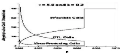
Figure 2: The phase diagram for model variables as a function of the parameter k withτ = 5.0 andp= 0.001.
Various model parameters are as in Table 1.
From Figure 1 we find that small values of delay fac-tor enhances and elongate the initial oscillations in the time series solutions of model variables. But there exist a threshold delay beyond which oscillations in variables smeared away and with increasing τ such smearing be-comes progressively fast. In Figure 2, we present the phase diagram of model variables as a function of the parameter p with τ = 5.0 andk = 0.2. Here we find a threshold value ofpbeyond which asymptotic stable so-lutions for y andz die-down and the same forxrises to its global stable value.
7
Discussion and conclusion
We have considered a basic mathematical model to rep-resent the virus dynamics of a HIV-1 infected individual including its response to RTI therapies. The RTI drugs actually impair the HIV-1 infected cells by inhibiting verse transcription of viral RNA into DNA, thereby re-ducing the rate of infection of uninfected T-cells. Our focus is to explore the effect of delay on the sustainable reduction of virus load in the system.
In our analytical studies on the HIV-1 dynamics we focus on the qualitative aspects of the HIV-1 dynamics within the model. Our calculations reveal that the existence and uniqueness of the solutions of dynamical variables x, y, and z locally holds in the positive octant. Through the local stability analysis we obtain sufficient conditions for the nonexistence of delay induced instability. The con-ditions obtained point towards the existence of asymp-totic stability of interior equilibrium. We have estimated the length of delay for which the stability of the sys-tem remains preserved. We find that delay assuming val-ues within the estimated length, Nyquist criteria holds. When the delay is set to the value beyond the estimated length, stable equilibrium solutions are seen bifurcate into small amplitude periodic solutions of Hopf type.
Numerical calculations reveal that delay affects consider-ably the attainability of the reduction of viral load in the HIV-1 infected system. Note that in the present model the reduction of the infected proportion of T-cells actu-ally means the reduction of viral load.
From discussion of the analytical and numerical solutions of the model it is clear that delay in the death rate of virus producing T-cells enhances oscillations in the model
variables, but asymptotically solutions are always stable. Further for definite set of choice of parametersp, k, andτ
the system moves to globally stable regime where sustain-ability of the reduction of the virus load is undoubtedly assured. Thus we can predict that if the application of RTI drugs are improvised at a optimum level in such a manner so as to match the parameters, killing rate of infected T-cells by CTL (p) at 0.001 mm3 /virus stim-ulation rate of CTL (k at 0.2) and delay in the death rate of infected T-cells (τ) at around 11 days then the possibility of eradication of HIV-1 in an individual and thereby restoration of healthy immune system would also be possible.
References
[1] Nowak, M. A., May, R. M., 1993,“ AIDS pathogenis: Mathematical models of HIV and SIV infections,”
AIDS, V7, pp.S3-S18.
[2] Le Corfec, E., Le Pont, F., Tuckwell, H. C., Rouzious, C., Costagliola, D., 1999, “Direct HIV testing in a blood donations; variation of the yield with diction threshold and pool size,” Transfusion, V39, pp.1141-1144.
[3] Perelson, A. S., Neuman, A. U., Markowitz, J. M. Leonard and Ho, D. D. 1996,“ HIV 1 dynamics in vivo: viron clearance rate, infected cell life span, and viral generation time,”Science, V271, pp.1582-1586.
[4] Sebastian Bonhoeffer, John M. Coffin, Martin A. Nowak, 1997, “Human Immunodeficiency Virus Drug Therapy and Virus Load,” Journal of Virol-ogy., V71, pp. 3275-3278.
[5] Coffin,J. M , 1995,“ HIV population dynamics in vivo: implications for genetic variation, pathogen-esis, and therapy,”Science, V267, pp. 482-489.
[6] Gopalsamy, K., 1992, Stability and Oscillations in Delay Differential Equations of Population dynam-ics, Kluwer Academic.
[7] Freedman,H.I., Erbe, L.H. and Rao, V.S.H., 1986,“ Three species food chain models with mutual inter-ference and time delays,”Math. Biosci., V80, pp.57-80.
[8] Marsden, J.E. and Mc Cracken, M. 1976,The Hopf Bifurcation and its application, Springer-Verglas, New York.
[9] Perelson, A. S., Krischner, D. E, De-Boer, R., 1993,“ Dynamics of HIV infection of CD4 T cells,” Math. Biosc., V114, pp.81-125.