ISSN 0001-3765 www.scielo.br/aabc
Short and long period optimization of drug doses in the treatment of AIDS
MARCO A. L. CAETANO1 and TAKASHI YONEYAMA2 1Departamento de Estatística, Matemática Aplicada e Computação Universidade Estadual Paulista, UNESP, 13.500-230 Rio Claro, SP, Brasil 2Divisão de Engenharia Eletrônica, Instituto Tecnológico de Aeronáutica, ITA
12.228-900 S.J. Campos, SP, Brasil
Manuscript received on March 26, 2001; accepted for publication on April 7, 2002; presented byCésar Camacho
ABSTRACT
Numerical optimization techniques are useful in solving problems of computing the best inputs for systems described by mathematical models and when the objectives can be stated in a quantitative form. This work concerns the problem of optimizing the drug doses in the treatment of AIDS in terms of achieving a balance between the therapeutic response and the side effects. A mathematical model describing the dynamics of HIV viruses and CD4 cells is used to compute the short term optimal drug doses in the treatments of patients with AIDS by a direct method of optimization using a cost function of Bolza type. The model parameters were fitted to actual published clinical data. In order to simplify the numerical procedures, the control law is expressed as a series and the sub-optimal control is obtained by truncating the higher terms. When the patient reaches a clinically satisfactory state, the LQR – Linear Quadratic Regulator technique is used to determine the long period maintenance doses for the drugs. The doses computed using the LQR technique tend to be smaller than equivalent constant-dose therapy in terms of increase in the counts of CD4+T cells and reduction of the density of free viruses.
Key words:modeling, simulation, drugs, treatment, AIDS.
INTRODUCTION
Quantitative descriptions of the dynamics exhibited by AIDS is now available as a consequence of intense clinical research, together with advances in the mathematical modeling methods: (Nowak and Bangham 1996, Phillips 1996, Perelson et al. 1993, Tan and Wu 1998). These mathematical
models can be used to optimize the drug doses required in the treatment. The model used in this work was proposed by Tan and Wu (Tan and Wu 1998), and is similar to Perelson (Perelson et al. 1993). The model paremeters are fitted using the actual clinical data found in Pontesilli et al. (1999).
This mathematical model comprises four differential equations representing the uninfected CD4+T cells, latent infected CD4+T cells, active infected CD4+T cells and free viruses.
At present, one of the most popular treatment scheme is HAART (highly active antiretro-viral therapy) which uses an association of reverse transcriptase inhibitors (eg. zidovudineand
lamivudine) and protease inhibitors (eg. saquinavir,indinavirandritonavir). After several months of treatment with those drugs, some patients have experienced increase in the side effects such as abdominal girth, abdominal fullness, distention or bloating (Mittler et al. 1998). Others pa-tients reported adverse effects such as headache, malaise, fatigue, nausea, vomiting, cough, nasal symptoms and musculoskeletal pain.
The effectiveness of a particular treatment scheme must be measured in an objective manner. One possibility is to construct a cost function that takes into account the number of non-infected CD4 cells and the administered doses of the drugs. The CD4 cells indicate the effectiveness of the treatment, while the doses of the administered drugs reflect the intensity of the side effects. Once the system model and the cost function are chosen, a variety of optimization techniques can be invoked to compute the best treatment scheme.
It was shown in a previous work (Caetano and Yoneyama 1999a) that it is possible to improve the treatment effectiveness by using a closed loop drug administration strategy. It was also shown (by computer simulation) that it is possible to use optimal control theory to minimize the side effects during a short term treatment scheme. However, the problem becomes hard to solve numerically when long term treatment is to be optimized. Here, after the patient reaches a clinically satisfactory state, a long term maintenance scheme is proposed based on Linear Quadratic Regulator theory (LQR). Small changes in the patient’s state are compensated using small changes in the drug doses that are optimal in the sense of minimizing a quadratic type performance index. The LQR control is widely used in the engineering area and references may be found, for instance, in Lewis (1986) and Kirk (1970).
MATERIALS AND METHODS
The Dynamic Model
of immunotherapy starting at different times after infection. In (Nowak and Bangham 1996) three dynamic models of HIV infection are compared. The first is the simplest and contains three variables x, y and v denoting, respectively, uninfected cells, infected cells and free viruses. Another model uses four variables where the three first variables are the same x, y, v as before and the new variable z represents CTL lymphocytes. The last model has four variables and includes the variability of the viruses. The model by Phillips (1996) involves four differential equations in variables R, L, E and V which represent, respectively, uninfected CD4, latent infected cells, infected cells and free virions. This model can be used to simulate the initial phase of infection. The model in (Nowak et al. 1995) considers the interaction between CTL and the multiple epitopes of a genetically variable pathogen. The version proposed in (Nowak et al. 1997) includes a population of mutant viruses, and provides analytic approximation for the rate of emergence of resistant viruses. This model comprises five equations and the results match the experimental data of three infected patients treated with Neverapine (NVP). In (Murray et al. 1998), the proposed model uses eight differential equations with the variables that represent the naïve cells. The model in (Wick 1999) takes into account the dynamics of T cells in which rising activation rates yield decreasing T cell counts and where apoptosis and proliferation must nearly balance. This model has four differential equations describing the dynamics of naïve T cells and memory cells in active and latent states. The model in (Zaric et al. 1998) focuses on the simulation of protease inhibitors and development of drug-resistant HIV strains. The model is composed of eleven differential equations, including couplings between organisms that are infected with resistant and non-resistant HIV strains. The model in (Tan and Wu 1998 and Tan and Xiang 1999) describe the HIV pathogenesis under treatment by antiviral drugs. The model has four differential equations and stochastic terms in the variables that represent the number of latent infected T cells. It has also stochastic components on infectious free HIV and non-infectious free HIV variables.
The mathematical model used in this work is a simplification of a more general version that includes stochastic terms, as originaly presented by (Tan and Wu 1998). The dynamics is described by the differential equations
˙
x1 =S(x4)+λ(x1, x2, x3)x1−x1{µ1+k1(m1)x4} ˙
x2 =ωk1(m1)x4x1−x2{µ2+k2(m2)} ˙
x3 =(1−ω)k1(m1)x4x1+k2(m2)x2−µ3x3 ˙
x4 =N (t )µ3x3−x4{k1(m1)x1+µv}
(1)
wherex˙ represents the time derivative dx/dt,
S(x4)= sθ θ +x4
(2)
λ(x1, x2, x3)=r
1− x1+x2+x3 Tmax
(3)
withx1 = x1(t ) ≡uninfected CD4+ T cells;x2 = x2(t ) ≡latent infected CD4+ T cells; x3 = x3(t )≡active infected CD4+T cells;x4=x4(t )≡free viruses HIV;s: rate of generation ofx1from precursors;r: rate of stimulated growth ofx1;Tmax: maximum T cells population level;µ1: death rate ofx1;µ2: death rate ofx2;µ3: death rate ofx3;µv: death rate ofx4;k1: infection rate from x1tox2by viruses;k2: conversion rate fromx2tox3;N: number of infectious virions produced by an actively infected T cell;θ: viral concentration needed to decreases. The coefficientsk1and k2are functions of the drug doses
k1(m1)=k10e−α1m1 (5) k2(m2)=k20e−α2m2 (6)
wherek10,k20,α1andα2are constants.
Basically,x1cells are stimulated to proliferate with rateλ(x1, x2, x3)in the presence of antigen and HIV (equation 3). Without the presence of HIV, the rate of generation isS(x4)(equation 2). In the presence of free HIV(x4), uninfected cellsx1can be infected to becomex2cells orx3cells, depending on probability of the cells to become actively or latently infected with rateω. Thex2 cells can be activated to becomex3cells. The activation rate isk2. Thex3cells are short living and will normally be killed upon activation with death rateµ3. Thex1,x2cells andx4free viruses have finite life and the death rates in this model areµ1,µ2andµvrespectively. Whenx3cells die, free virusesx4are released with rateN (t )described by (4). Drugs such as reverse transcriptase inhibitors (zidovudineandlamivudine) and protease inhibitors (saquinavir,indinavirandritonavir) affect the dynamics via parametersk1andk2.
The Sub-optimal Control
The objective in a general optimal control problem is to find a control inputm(t )= [m1(t )m2(t )]T that minimizes the cost function
J[m] =h(x(tf), tf)+ tf
t0
g(x(t ), m(t ), t )dt (7)
wheret0andtf are the initial and final times, fixeda priori. The functionshandgare required to be positive. Moreover,x(·)andm(·)are constrained by the state equation
˙
x =f (x(t ), m(t ), t ) (8)
In the specific problem treated in this work,x = [x1x2x3x4]t ∈Rnandm= [m1m2]t
f (x, m, t )=
S(x4)+λ(x1, x2, x3)x1−x1{µ1+k1(m1)x4} ωk1(m1)x4x1−x2{µ2+k2(m2)} (1−ω)k1(m1)x4x1+k2(m2)x2−µ3x3
N (t )µ3x3−x4{k1(m1)x1+µv}
k1(m1)=k10e−α1m1 (10)
k2(m2)=k20e−α2m2 (11)
h(x(tf), tf)=
γ1 x1(tf)
(12)
g(x(t ), m(t ), t )=φ1
1−exp−ε1m1(t )2
+φ2
1−exp−ε2m2(t )2
+ γ2 x1(t )
(13)
wherek10,k20,α1,α2,φ1,φ2,γ1,γ2,ε1andε2are constants.
The biological interpretation of the proposed cost functional is that the first termh(x(tf), tf) represent the target of maximizing non-infected CD4 after a pre-specified time horizon. The coefficients φ1 and φ2 in the integrandg(x(t ), m(t ), t ) are weights that reflect the dose-related side effects of the two drugs (m1andm2) which must be adequately balanced. The last term in g(x(t ), m(t ), t )is included to forcex1(uninfected CD4+T cells) to increase with treatment.
Optimal control problems can be solved by indirect or direct methods. In the solution using an indirect method, one is required to solve a boundary value problem with 2nequations corresponding to n state and n adjoint variables if Maximum Principle is invoked or to solve a partial differential equation if Dynamic Programming is used (Kirk 1970, Lewis 1986 and Bulirsh and Stoer 1980). In the solution using a direct method, one attempts to minimize directly the performance measure (7) after a suitable parametrization of the admissible control inputsm(t ). Here, a direct method proposed by Jacob (1972) is used. The parametrization of the input functionsm(t )involves, in the present case, a subset of the coefficients in the series expansion employing sine functions. Therefore, only approximations to the actual optimalm(t )can be obtained. Those approximations are sub-optimal, in the sense that the cost achieved is generally greater when the higher terms of the series expansion are neglected, compared to the case resulting from the use of the actual optimal control. However, those sub-optimal control inputs were found to be satisfactory in the present problem.
Parametrization of the Control Input
The numerical algorithm proposed in (Jacob 1972) is available in the form of a computer program called EXTREM. Each component of the control inputm(t )is represented by an expansion over the interval[0, tf]with the form
mi(t ) = c1,i+c2,isin(t π/tf),+c3,i
2 sin(t π/tf)cos(t π/tf)
+c4,i
3 sin(t π/tf)cos(t π/tf)2−sin3(t π/tf)
+ . . . + cni
(n−1)sin(t π/tf)cosn−2(t π/tf)−
(n−1)/3sin3(t π/tf)cosn−4(t π/tf)
+(n−1)/5sin5(t π/tf)cosn−6(t π/tf)−. . .+. . .
(14)
Linear Mathematical Model
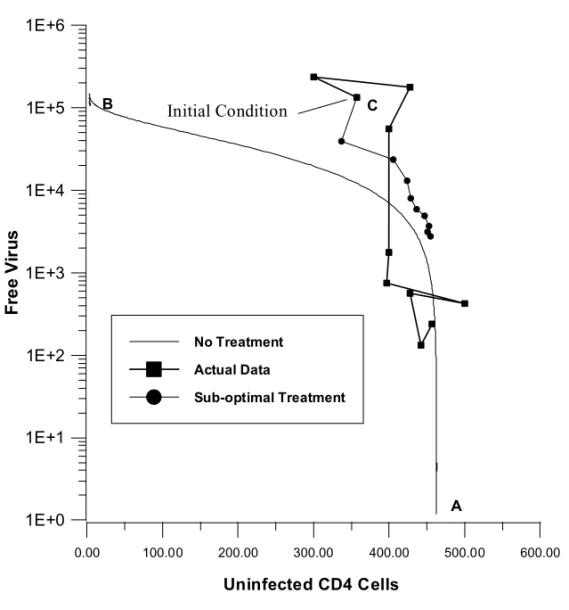
Once the patient’s state reaches a clinically satisfactory region after the sub-optimal short term treatment, the idea is to use the LQR (Linear Quadratic Regulator) as the long term treatment. In order to obtain a linearized model to be used within the clinically satisfactory region, the data corresponding to the patient A by (Pontesilli et al. 1999) is considered for illustration purposes. For other patients, the clinical data gathered before and during the short-term treatment is used to identify the numerical values of the parameters for the linearized model. The estimated numerical values for the model parameters of patient A are shown in Table I. The graph in Figure 1 shows the values determined by simulation and the actual data for the uninfected CD4+T cells and HIV free viruses of patient A by (Pontesilli et al. 1999). In the case of constant doses therapy, these were adjusted to be the same as in the actual treatment reported by Pontesilli, i.e., 900 mg of a transcriptase inhibitor and 1200 mg of a protease inhibitor during 224 days.
TABLE I
Model parameters used in the numerical simulations.
S R Tmax µ1 µ2 µ3 µv k10 k20 N0
10 0.52 1700 0.4 0.5 2.4 2.4 2.410-5 3.10-1 1400
φ1 φ2 ε1 ε2 γ1 γ2 α1 α2 θ ω
1 1 1.10-6 1.10-6 250.103 250.103 0.005 0.005 1.106 1
β1 β2 x1(0) x2(0) x3(0) x4(0) tf(days)
1.10-1 65470 357 10 100 133352 224
For this patient, with the parameters of Table I, one is able to find the equilibrium points by solving the equations (1) after lettingdx/dt =0:
S(x4)+λ(x1, x2, x3)x1−x1{µ1+k1(m1)x4} =0 ωk1(m1)x4x1−x2{µ2+k2(m2)} =0
(1−ω)k1(m1)x4x1+k2(m2)x2−µ3x3=0 N (t )µ3x3−x4{k1(m1)x1+µv} =0
(15)
The critical points for the patientAare found to be:
first point x∗ = (462.828;0;0;0)
second point x∗ = (4.07;13.1;131.04;107241) third point x∗ = (−70.62;0;0;0)
0.00 100.00 200.00 300.00 400.00 500.00 600.00
Uninfected CD4 Cells
1E+0 1E+1 1E+2 1E+3 1E+4 1E+5 1E+6
Fr
e
e
V
ir
us
Initial Condition
A
B C
No Treatment
Actual Data
Sub-optimal Treatment
Fig. 1 – Comparison between sub-optimal (computer simulation) and constant-dose treatment schemes (actual data). The point A indicates initial infection; B represents an advanced stage on AIDS without treatment; C represents the condition at the beginning of the sub-optimal treatment.
A local analysis of these points show that the first point is unstable while the second is stable. In fact, the eigenvalues of the linearized model at the first point are:
λ1= −2.13+1.35i λ2= −2.13−1.35i λ3=1.019
λ4= −0.163
(16)
and the eigenvalues at second point are:
λ1= −2.439+0.189i λ2= −2.439−0.189i λ3= −0.7747
λ4= −0.0319
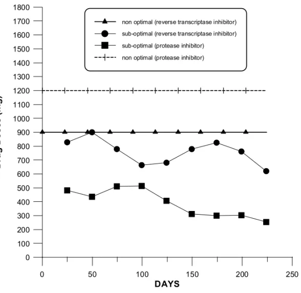
Therefore, the idea of using LQR scheme is to keep the patient’s state near the first critical point, which is unstable without feedback control. Initially, the patients use either sub-optimal or constant doses therapy of reverse transcriptase inhibitor plus protease inhibitor until the level of CD4+T is near to the first critical point, shown in Figure 2. For instance, after a short period constant doses treatment withm∗=(900,1200), the reached state is
x∗=(462.6639,0.0271,0.1247,103.3111)
0 50 100 150 200 250
DAYS
0 100 200 300 400 500 600 700 800 900 1000 1100 1200 1300 1400 1500 1600 1700 1800
Dr
u
g
Do
s
e
s
(m
g
)
non optimal (reverse transcriptase inhibitor)
sub-optimal (reverse transcriptase inhibitor)
sub-optimal (protease inhibitor)
non optimal (protease inhibitor)
Fig. 2 – Drug doses used in the computer simulations.
Now, it is possible to linearize the equations (1) about this state. Thus, for small perturbations near the critical point:
x1=x1∗+x1 x2=x2∗+x2 x3=x3∗+x3 x4=x4∗+x4
corresponding to small adjustments in the control variable (drugs doses)
m1=m∗1+m1
m2=m∗2+m2
(19)
and adopting an additional assumption of negleting the variations of the active and latent cells, one can write
x˙ = ∂f ∂x
(x∗,m∗)
x+ ∂f ∂m
(x∗,m∗)
m (20) or
x˙1 x˙2 x˙3 x˙4 =
r(1−2x1
T )−(µ1+k1x4) 0 0 −x1k1
k1x4 −(µ2+k2) 0 k1x1
0 k2 −µ3 0
−k1x4 0 N µ3 −(k1x1+µv)
(x∗,m∗)
x1 x2 x3 x4 +
x1x4k10e−α1m1 0 −x1x4k10e−α1m1 x2k20α2e−α2m2
0 −x2k20α2e−α2m2 x4x1α1k10e−α1m1 0
(x∗,m∗)
m1 m2
(21)
In the region of interest, the model becomes:
x˙1 x˙2 x˙3 x˙4
=
−0.165 0 0 −0.0111 0.0024 −0.8 0 0.0111
0 0.3 −0.03 0
−0.0024 0 42 −2.4111 x1 x2 x3 x4 +
0.00008644 0
−0.00008644 0.00001872 0 −0.00001872 0.00008644 0
m1 m2 (22)
and the observation equations, assuming that only CD4+T cells and free virus are monitored, becomes: y1 y2 =
The Linear Quadratic Regulator
The LQR is widely used in control engineering because of its simplicity and robustness properties. The action of the control variable is to minimize a performance index:
Minimize J = 1
2
+∞
0
x(t )TQx(t )+mT(t )Rm(t )dt (24)
subject to x˙ =Ax+Bm (25)
whereA,B,QandR are matrices of appropriate dimensions andRis positive definite.
The solution of the LQR problem is well known and can be found, for instance, in Lewis (1986) and Kirk (1970):
m(t )= −R−1BTP x(t ) (26)
whereP is to be found by solving the algebraic Riccati equation:
ATP +P A−P BR−1BTP +Q=0 (27)
TheQmatrix is the weight on the statesxandRmatrix is the weight on the control variable
m. The values ofQandR used here are:
Q =
10−6 0 0 0 0 1 0 0 0 0 1 0 0 0 0 1
R
=
5x10³ 0 0 102
(28)
A larger weight was placed on the reverse transcriptase inhibitor because the objective is to reduce the number of active infected cells.
RESULTS
The actual clinical data were extracted from Pontesilli et al. (1999) and refers to a patient (patient A) that contracted AIDS and his T cell counts were measured during 224 days. Firstly, the model parameters were adjusted by an identification procedure to match the available data. The model parameters are presented in Table I.
The control variables were constrained to be in the range (300 mg) ≤ m1(t ) ≤ (900 mg) reverse transcriptase inhibitor and(300 mg)≤m2(t )≤(900 mg)protease inhibitor, respectively, which are the same values proposed in Pontesilli et al. (1999).
in Pontesilli and the computer-generated sub-optimal response. Figure 1 also shows the path A– B followed by a recently infected patient with an infinitesimal quantity of viruses. The point C corresponds to the initial condition used in the simulations. The other components of the state (x2 andx3) are also close to the actual data. The doses in the case of sub-optimal treatment scheme are lower than the constant dose strategy, as seen in Figure 2.
In order to evaluate the long period maintenance doses for the drugs, the equations (8)–(11) were integrated assuming constant drug doses with values that equal those used in the treatment of patient A in (Pontesilli et al. 1999). After 224 days, the drug administration strategy was switched to the optimal control law based on LQR.
Figure 3 shows the results of the count of uninfected CD4+T cells and free viruses, respectively, under LQR drug doses. It is seen that the level of CD4+T increases while the free viruses are further reduced.
100 200 300 400 500
time (days) 460
470 480 490 500 510
C
D
4
(c
e
lls
/m
m
3
)
Start of LQR
0.00 0.01 0.10 1.00 10.00 100.00 1000.00
Fr
e
e
V
ir
u
s
(/m
m
3
)
CD4+T
Free Virus
Fig. 3 – CD4+T cells and Free Virus under LQR drug doses.
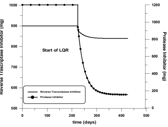
Figure 4 shows two curves correspondig to the case of a two phase treatment scheme, where in the short term the doses are kept constant and in the long term the LQR is used. The doses are seen to adjust themselves towards stationary values with a slight and progressive reduction of the reverse transcriptase inhibitor and a significant reduction of the protease inhibitor.
DISCUSSIONS AND CONCLUSIONS
0 100 200 300 400 500
time (days)
500 600 700 800 900 1000
R
e
v
e
rs
e
T
rasc
ri
p
tase
In
h
ib
it
o
r
(mg
)
Start of LQR
0 200 400 600 800 1000 1200
P
rot
e
a
s
e
Inh
ibi
tor
(m
g)
Reverse Transcriptase Inhibitor
Protease Inhibitor
Fig. 4 – Reverse Transcriptase and Protease Inhibitor under LQR.
drawback is the necessity to estimate the model parameters for each patient, which may be a formidable task. However, simulation studies carried out with clinical data indicate that even models with considerable uncertainty can yield useful results. The sub-optimal treatment scheme may produce inferior results when compared to the actual optimal scheme, but in view of the subjective nature of the cost function and of the required computational effort, the approximation obtained by the proposed method may still be adequate. An interesting fact is that for other patients reported in Pontesilli, (patients B, C and D) the proposed method yields good numerical results obtained by computer simulation.
that the much simpler LQR method can be used to compute the doses for the long term treatment. Moreover, because of the usual robustness properties of the LQR regulator, the controller tends to be less sensitive to modeling errors (Lewis 1986).
RESUMO
Técnicas de otimização numérica são úteis na solução de problemas de determinação da melhor entrada
para sistemas descritos por modelos matemáticos e cujos objetivos podem ser expressos de uma maneira
quantitativa. Este trabalho aborda o problema de otimizar as dosagens dos medicamentos no tratamento da AIDS em termos de um balanço entre a resposta terapêutica e os efeitos colaterais. Um modelo matemático
para descrever a dinâmica do vírus HIV e células CD4 é utilizado para calcular a dosagem ótima do
medica-mento no tratamedica-mento a curto prazo de pacientes com AIDS por um método de otimização direta utilizando
uma função custo do tipo Bolza. Os parâmetros do modelo foram ajustados com dados reais obtidos da
literatura. Com o objetivo de simplificar os procedimentos numéricos, a lei de controle foi expressa em
termos de uma expansão em séries que, após truncamento, permite obter controles sub-ótimos. Quando os
pacientes atingem um estado clínico satisfatório, a técnica do Regulador Linear Quadrático (RLQ) é utilizada
para determinar a dosagem permanente de longo período para os medicamentos. As dosagens calculadas
utilizando a técnica RLQ , tendem a ser menores do que a equivalente terapia de dose constante em termos
do expressivo aumento na contagem das células T+CD4 e da redução da densidade de vírus livre durante
um intervalo fixo de tempo.
Palavras-chave: modelamento, simulação, medicamentos, tratamento, AIDS.
REFERENCES
Behrens DA, Caulkins JP, Tragler G, Haunschmied JL and Feichtinger G.1999. A dynamic model
of drug initiation: implications for treatment and drug control. Mathematical Biosciences 159: 1–20.
Bulirsh R and Stoer J.1980. Introduction to Numerical Analysis. Springer-Verlag. 609 p.
Caetano MAL and Yoneyama T.1999a. Comparative Evaluation of Open Loop and Closed Loop Drug
Adminstration Strategies in the Treatment of AIDS. An Acad Bras Cienc 71 4-I: 589–597.
Caetano MAL and Yoneyama TA.1999b. Optimal Control Theory Applied to the Anti-Viral Treatment
in AIDS. 4thESMTB – Theory and Mathematics in Biology and Medicine, Amsterdam pp. 113–117.
Felippe de Souza JAM, Caetano MAL and Yoneyama T.2000. Numerical Optimization Applied to
the Treatment of AIDS in the Presence of Mutant HIV Virus. 4thIFAC Symp. Modelling and Control. Greifswald. Germany. 91–96.
Jacob HG. 1972. An Engineering Optimization Method with Application to Stol Aircraft Aproach and
Landing Trajectories. Langley. NASA TN-D 6978. 38 p.
Kirk DE.1970. Optimal Control Theory: an Introduction. Prentice-Hall . New Jersey. 452 p.
Math Biol 58: 376–390.
Kirschner D, Lenhart S and Serbin S.1997. Optimal Control of the Chemotherapy of HIV. J Math.
Biol 35: 775–792.
Lewis FL.1986. Optimal Control. John Wiley. New York. 362 p.
Mittler JE, Sulzer B, Neumann AU and Perelson AS.1998. Influence of delayed viral production
on viral dynamics in HIV-1 infected patients. Mathematical Biosciences 152: 143–163.
Murray JM, Kaufmann G, Kelleher AD and Cooper DA.1998. A Model of primary HIV-1 infection.
Mathematical Biosciences 154: 57–85.
Nowak MA and Bangham CRM.1996. Population Dynamics of Immune Responses to Persistent Viruses.
Science 272: 74–79.
Nowak MA, Anderson RM, McLean AR, Wolfs TF, Goudsmit J and May RM. 1991. Antigenic
Diversity Thresholds and the Development of AIDS. Science 254: 963–969.
Nowak MA, May RM, Phillips RE, Jones SR, Lallo DG, McAdams S, Klenerman P, Köppe B,
Sigmund K, Bangham CRM and McMichael AJ.1995. Antigenic oscillations and shifting
immun-odominance in HIV-1 infections. Nature 375: 606–611.
Nowak MA, Bonhoeffer S, Shaw GM and May RM.1997. Anti-viral Drug Treatment: Dynamics of
Resistence in Free Virus and Infected Cell Populations. J Theoretical Biology 184: 203–217.
Perelson AS, Kirschner DE and DeBoer R.1993. Dynamics of HIV-infection of CD4+T-cells.
Math-ematical Biosciences 114: 8–125.
Phillips A.1996. Reduction of HIV Concentration During Acute infection; Independence from a Specific
Immune Response. Science 271: 497–499.
Pontesilli O, Kerkhof-Garde S, Pakker NG, Notermans DW, Roos MTL, Klein MR, Danner SA
and Miedema F.1999. Immunology Letters 66: 213–217.
Tan WY and Wu H.1998. Stochastic Modeling of the Dynamics of CD4+T-Cell Infection by HIV and
Some Monte Carlo Studies. Mathematical Biosciences 147: 173–205.
Tan WY and Xiang Z.1999. Some state space models of HIV pathogenesis under treatment by anti-viral
drugs in HIV-infected individuals. Mathematical Biosciences 156: 69–94.
Wein LM, D’Amato RM and Perelson A.1998. Mathematical Analysis of Antiretroviral Therapy Aimed
at HIV-1 Eradication or Maintenance of Low Viral Loads. J Theoretical Biology 192: 81–98.
Wick D.1999. On T-cell dynamics and the hyperactivation theory of AIDS pathogenesis. Mathematical
Biosciences 158: 127–144.
Zaric GS, Bayoumi AM, Brandeau ML and Owens DK.1998. The Effects of Protease inhibitors on