INTEGRATION OF REAL TIME OPTIMIZATION (RTO) AND MODEL
PREDICTIVE CONTROL (MPC) OF AN INDUSTRIAL
PROPYLENE/PROPANE SPLITTER
INTEGRATION OF REAL TIME OPTIMIZATION (RTO) AND MODEL
PREDICTIVE CONTROL (MPC) OF AN INDUSTRIAL
PROPYLENE/PROPANE SPLITTER
Tese apresentada à Escola Politécnica da Universidade de São Paulo para obtenção do título de Doutor em Ciências
Orientador: Prof. Dr. Darci Odloak
INTEGRATION OF REAL TIME OPTIMIZATION (RTO) AND MODEL
PREDICTIVE CONTROL (MPC) OF AN INDUSTRIAL
PROPYLENE/PROPANE SPLITTER
Tese apresentada à Escola Politécnica da Universidade de São Paulo para obtenção do título de Doutor em Ciências
Área de Concentração: Engenharia Química
Orientador: Prof. Dr. Darci Odloak
Primeiro agradecer a Deus pela vida e a oportunidade de completar um sonho e recobrar a saúde. A minha esposa Rosita e toda minha família na Bolívia pelo apoio incondicional durante todos esses anos de estudo, por torcer e confiar sempre em mim.
Ao Prof. Darci Odloak pelo conhecimento transmitido, comentários, sugestões, amizade, por confiar em mim e me dar a oportunidade de trabalhar com controle preditivo de processos.
À Profa. Rita Alves pelo primeiro contato, apoio e pela amizade desde que cheguei a São Paulo.
Ao pessoal da Invensys por facilitar a licença acadêmica para o uso de software para a realização deste trabalho e pelas dicas no uso correto do software, em especial, Erika Fernandez, Rubens Rejowski e Neliana Azacón.
À minha banca examinadora da qualificação e pessoal da Petrobras pela informação e criticas construtivas para realizar este projeto, em especial, Dr. Antonio Carlos Zanin (CETAI), Prof. Galo Le Roux e Eng. Carlos Henrique (RECAP).
Aos Professores do Departamento de Engenharia Química por transmitir os conhecimentos e ferramentas para concluir este trabalho.
Aos meus amigos da SJB, Eduardo, Nedher, Juancho, Ana, Roxana, Sandra pelos bons momentos que compartilhamos e por estar comigo nos momentos mais difíceis.
Aos amigos do Laboratório de Simulação e Controle de Processos (LSCP) pela amizade e pelas conversas na copa do Bloco 21, em especial, Brunos, André, Daniel (Dorminhoco), Ricardo, Álvaro, Zés e Marion.
The die is cast and you can’t restart or change the past, but if given only one more chance, could you carve the way?
I’m sick of being afraid and living by these mistakes that I have made, but I’ll change that with these hands of mine.
Believing in something more, I’ll carve a path through that rusted doorway. There’s still more that’s still worth fighting for, so take aim and don't wait or hesitate.
O propósito desta Tese é realizar o estudo da implementação do controle avançado do tipo controle preditivo baseado em modelo (MPC) e otimização em tempo real (RTO) em uma unidade de processo industrial usando como ferramentas softwares
comerciais de simulação e otimização de processos. As soluções propostas podem ser consideradas como estratégias de integração entre RTO e MPC de uma e duas camadas.
Na estratégia de duas camadas, a camada superior que considera um modelo rigoroso não linear do processo computa e envia targets otimizantes à camada
dinâmica do MPC, que computa as ações de controle necessárias para alcançar esses targets e estabilizar o processo. Na estratégia de uma camada, mais
conhecida como MPC econômico, temos a inclusão do gradiente da função econômica na função custo do controlador preditivo.
Ambas as estratégias foram estudadas e suas implementações na coluna de destilação de propeno/propano com integração energética da unidade de produção de propeno da refinaria de Capuava da Petrobras foram simuladas. Este estudo foi realizado em varias etapas. Primeiro, uma simulação dinâmica do processo foi realizada usando o simulador dinâmico SimSci Dynsim® para ser usada como uma planta virtual que também foi usada para a identificação dos modelos usados nos controladores preditivos. Segundo, os algoritmos de controle avançado foram desenvolvidos em Matlab® baseados no controlador preditivo de horizonte infinito (IHMPC), no controlador preditivo robusto (RIHMPC) e no MPC econômico. Terceiro, o algoritmo de RTO foi desenvolvido no pacote de otimização em tempo real Simsci ROMeo®, onde o modelo rigoroso não linear do processo foi implantado incluindo as etapas de simulação, reconciliação de dados e otimização. Quarto, modificações e adaptações dos algoritmos e rotinas desenvolvidas foram feitas para permitir a comunicação de dados em tempo real usando o protocolo de transferência de dados OPC entre Matlab®, Simsci Dynsim® e Simsci ROMeo®. Finalmente, foram desenvolvidos o sequenciamento e automação dos algoritmos tanto para leitura e escritura de dados, assim como, para a rotina do RTO.
Para todas as estratégias propostas nesta Tese, foram incluídos exemplos de simulação representativos onde se pode evidenciar a estabilidade e convergência das estratégias propostas, chegando-se à conclusão que as estruturas propostas de RTO/MPC podem ser implementadas no sistema real.
The aim of this Thesis is to study the implementation of advanced control, specifically, Model Predictive Control (MPC) and real time optimization (RTO) in an industrial process system using tools such as commercial software for process simulation and optimization. The proposed solutions can be considered as integration strategies of RTO and MPC with one and two layers.
In the two layer approach, the upper layer that considers a rigorous non-linear steady-state model of the process computes optimizing targets that are sent to the dynamic layer that are based on the MPC, which computes the necessary control actions to reach those targets and stabilize the process system. In the one layer strategy, also called as Economic MPC, the gradient of the economic function is included in the cost function of the predictive controller.
Both strategies were studied and their implementation in the energy-recovery propylene/propane splitter system of the propylene production unit at the Capuava Refinery of Petrobras was simulated. In order to accomplish this objective, the work was developed in several steps. Firstly, a dynamic simulation of the process was built in the dynamic simulator Simsci Dynsim® so that it could be used as a virtual plant in which the model identification could also be performed. Secondly, the advanced control algorithms were developed in Matlab® based on the Infinite Horizon Model Predictive Control (IHMPC), the robust predictive controller (RIHMPC) and the Economic MPC. Thirdly, the RTO algorithm was developed in the real-time optimization package Simsci ROMeo®, where the non-linear rigorous model of the process was built including the stages of simulation, data reconciliation and optimization. Fourthly, modifications and adaptation of the developed algorithms and routines were included to allow the real-time data communication considering the OPC data transfer protocol between Matlab®, Dynsim® and ROMeo®. Finally, a sequence of algorithms was developed and automated for data reading and writing, as well as, for the RTO sequence.
For all the strategies developed in this Thesis, representative simulation examples were presented in order to show the closed-loop stability and convergence of the proposed approaches, leading to the conclusion that the proposed RTO/MPC structures can be implemented in the real system.
Figure 2. 1 – Two-layer hierarchical structure without RTO ... 22
Figure 2. 2 – Two-layer hierarchical structure with RTO ... 23
Figure 2. 3 – Three-layer hierarchical structure with RTO ... 23
Figure 2. 4 – One-layer hierarchical structure (Economic MPC) ... 25
Figure 2. 5 – ROMeo’s internal modules (ROMeo User Guide, 2012) ... 27
Figure 3. 1 – Schematic representation of the Propylene/Propane splitter ... 33
Figure 3. 2 – Snapshot summary of the PP Splitter in Dynsim ... 47
Figure 3. 3 – PFD of the PP Splitter in Dynsim ... 48
Figure 4. 1 – Selected manipulated and controlled variable for step response test ... 49
Figure 4. 2 – Step responses of the PP splitter at different operating points ... 50
Figure 5. 1 – PFD of the PP splitter in Simulation mode in ROMeo ... 79
Figure 5. 2 – PFD of the PP splitter in Data reconciliation mode in ROMeo ... 81
Figure 5. 3 – SSD task in ROMeo RTS ... 86
Figure 5. 4 – Model Sequence in ROMeo RTS ... 86
Figure 5. 5 –Sensitivity analysis tool in ROMeo OPS ... 88
Figure 6. 1 – Two layer structure strategy ... 89
Figure 6. 2 – Controlled outputs IHMPC (First experiment) ... 93
Figure 6. 3 – Manipulated inputs IHMPC (First experiment) ... 94
Figure 6. 4 – Economic function IHMPC (First experiment) ... 94
Figure 6. 5 – Economic function IHMPC with penalization (First experiment) ... 95
Figure 6. 6 – Controlled outputs IHMPC (Second experiment) ... 96
Figure 6. 7 – Manipulated inputs IHMPC (Second experiment) ... 96
Figure 6. 8 – Economic function IHMPC (Second experiment) ... 97
Figure 6. 9 – Economic function IHMPC with penalization (Second experiment) ... 97
Figure 6. 10 – Controlled outputs (First experiment) ... 99
Figure 6. 11 – Manipulated inputs (First experiment) ... 100
Figure 6. 12 – Economic function (First experiment) ... 100
Figure 6. 13 – Economic function with penalization (First experiment) ... 101
Figure 6. 14 – Controlled outputs (Second experiment) ... 102
Figure 6. 15 – Manipulated inputs (Second experiment) ... 103
Figure 6. 16 – Economic function (Second experiment) ... 103
Figure 6. 17 – Economic function with penalization (Second experiment) ... 104
Figure 6. 18 – One layer structure solution ... 105
Figure 6. 19 – Controlled outputs (First experiment) ... 106
Figure 6. 20 – Manipulated inputs (First experiment) ... 106
Figure 6. 21 – Economic function (First experiment) ... 107
Figure 6. 22 – Economic function with penalization (First experiment) ... 107
Figure 6. 23 – Controlled outputs (Second experiment) ... 109
Figure 6. 24 – Manipulated inputs (Second experiment) ... 109
Figure 6. 25 – Economic function (Second experiment) ... 110
Figure 6. 26 – Economic function with penalization (Second experiment) ... 110
Table 3. 1 – Typical feed composition of propylene/propane splitter ... 32
Table 3. 2 – Column T-03 description ... 34
Table 3. 3 – Heat exchangers M-01 A/B description ... 35
Table 3. 4 – Heat exchanger M-02 description ... 36
Table 3. 5 – Heat exchangers M-03 A/B description ... 36
Table 3. 6 – Heat exchanger M-04 description ... 37
Table 3. 7 – Drum O-01 description ... 37
Table 3. 8 – Separator O-02 description ... 38
Table 3. 9 – Drum O-03 description ... 38
Table 3. 10 – Drum O-04 description ... 39
Table 3. 11 – Valve coefficients (Cv) ... 42
Table 3. 12 – Overall heat transfer coefficients ... 42
Table 3. 13 – Compressor V-01 curves ... 43
Table 3. 14 – Dynamic equipment data T-03 ... 43
Table 3. 15 – Main PID controllers used in the propylene/propane splitter ... 44
Table 3. 16 – Main PID controller tuning ... 45
Table 4. 1 – Different operating conditions of the PP splitter... 50
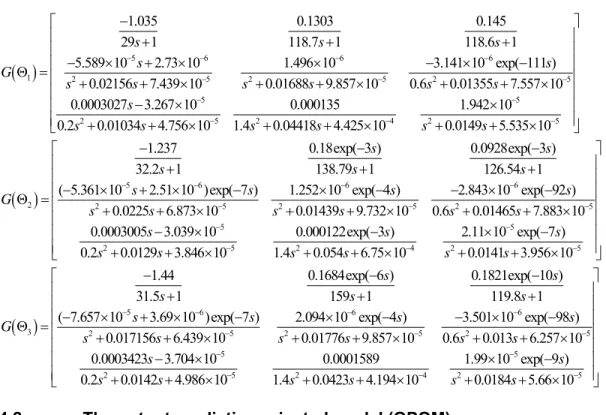
Table 4. 2 – Transfer function models of the PP splitter ... 52
Table 6. 1 – Output zones of the propylene/propane splitter ... 90
Table 6. 2 –Input constraints of the propylene/propane splitter ... 90
Table 6. 3 – Feed molar composition (Disturbance) ... 91
Table 6. 4 – IHMPC-OPOM tuning parameters ... 92
Table 6. 5 – IHMPC-Realignment model maximum input moves ... 92
Table 6. 6 – IHMPC-Realignment model tuning parameters ... 93
Table 6. 7 – Robust MPC tuning parameters ... 99
Acronyms and Abbreviations
ROMeo Rigorous Online Modeling with equation-based optimization Dynsim Dynamic Simulation
MPC Model Predictive Control RTO Real Time Optimization
IHMPC Infinite Horizon Model Predictive Control
RIHMPC Robust Infinite Horizon Model Predictive Control DOF Degrees of Freedom
PFD Process Flow Diagram QP Quadratic Programming
LP Linear Programming
DMC Dynamic Matrix Control
LDMC Linear Dynamic Matrix Controller MATLAB Matrix Laboratory
DCS Distributed Control System NLP Non Linear Programming OPC OLE for Process Control
OMPC Optimizing Model Predictive Control PID Proportional, Integrative and Derivative OPOM Output Predictive Oriented Model PP Propylene/Propane
SSD Steady State Detection DataRec Data Reconciliation SICON Control System
DA Data Acquisition
EDI External Data Interface Roman Symbols
0 Null matrix of any dimension
A State transition matrix
A Auxiliary matrix used in the state and output prediction B Matrix that relates system inputs and states
B Auxiliary matrix used in the calculation of output prediction d
l
B Matrix that relates the control actions with the state component xd s
l
B Matrix that relates the control actions with the state component xs C Matrix that relates the states to the system outputs
0 ,
i j
d Gain of the transfer function Gi j,
, ,
d i j k
d k-nth residual of the transfer functionGi j, d
D Matrix that concentrates all di j kd, ,
e Error between the real and estimated state
feco Economic function of the system
F Matrix with the dynamic of the stable modes ( )
G s Transfer function that represents the system to be controlled
m Control horizon
p Prediction horizon
n
I Identity matrix of dimension n
nu
I Auxiliary matrix used in the formulationof input constraints
ny
I Auxiliary matrix used in computation of the cost function contribution of the deviation between outputs and control zones
J Auxiliary matrix to relate control actions and components d l B
L Gain of the state corrector used in the realigned IHMPC
na Transfer function orders of Gi j, ( )s nd Dimension of component xd(
nd nu ny na )
d
N (Ns) Matrix used to extract component d x (xs)
nu Number of system inputs
ny Number of system outputs
u
Q Weight in the controller objective function of the deviation between the inputs and the optimizing targets
y
Q Weight in the controller objective function on the deviation between the outputs and their control zones
, , i j k
r kth pole of the transfer functionGi j, ( )s
R Weight used in the controller cost function for the suppression of
control actions
, ,
i u y
S S S Weight matrix in the controller cost function of the slack variables , , , , ,
i k u k y k
t Time
T Sampling time
u Vector of system inputs
des
u Optimizing targets for the system inputs max
u Upper constraint of the system inputs min
u Lower constraint if the system inputs
k
V Total cost of the controller objective function at time k x Vector containing the system states
d
x Vector that computes the evolution of the system stable modes s
x System output prediction at steady-state y Vector of the system outputs
( | )
y ki k Prediction at time k of the system output at time ki min
,
sp k
y Set-point computed by the controller at time k
l
z State that stores the control actions implemented in the l previous
sample instants
Greek Symbols
Slack variable
,
u k
Slack variable for the deviation between the system inputs and the optimizing targets
,
y k
Slack variable for the deviation between the system outputs and the computed set-points
u
Input move(Control action)
k
u
Vector of control actions computed for all control horizon m
max u
Maximum admissible input move
max U
Vector containing the input moves for all the control horizon m
eco
f
Gradient of the economic function feco
,
i j
Time delay for the transfer functionGi j, ( )s
max
Biggest time delay of the system transfer function Gi j, ( )s
, ,
i j k
kth coefficient of the partial fraction expansion of transfer function , ( )
i j
G s
Auxiliary matrix for the construction of
1 INTRODUCTION ... 16
1.1 Advanced control and Real-time optimization ... 16
1.2 Motivation ... 18
1.3 Objectives ... 19
1.4 Organization of the thesis ... 19
1.5 Publications ... 20
1.5.1 Published paper ... 20
1.5.2 Submitted paper ... 20
1.5.3 Participation in conferences ... 20
1.5.4 Awards ... 21
2 LITERATURE REVIEW ... 22
2.1 Model predictive control and Real time Optimization ... 22
2.2 Process simulation ... 26
2.2.1 Steady-state modeling and optimization using ROMeo® ... 27
2.2.2 Dynamic simulation ... 28
2.3 Real time data communication... 29
2.3.1 Open platform communications (OPC) ... 29
2.3.2 MATLAB OPC toolbox ... 30
3 HIGH PURITY DISTILLATION PROCESS AND DYNAMIC SIMULATION DEVELOPMENT ... 32
3.1 Process description ... 32
3.2 Equipment description ... 34
3.2.1 Depropenizer splitter (T-03) ... 34
3.2.2 Propylene compressor (V-01) ... 35
3.2.3 Heat exchangers ... 35
3.2.3.1 Reboilers M-01 A/B ... 35
3.2.3.2 Reboiler M-02 ... 35
3.2.3.3 Cooler M-03 A/B ... 36
3.2.3.4 Cooler M-04 ... 36
3.2.4 Drums and separators ... 37
3.2.4.4 Drum O-04 ... 39
3.3 Existing multivariable advanced controller (LDMC) ... 39
3.3.1 Controlled variables (Outputs) ... 39
3.3.2 Manipulated variables (Inputs) ... 40
3.4 Dynamic simulation of the PP Splitter ... 41
3.4.1 Equipment description for the dynamic simulation ... 41
3.4.2 Valve coefficients ... 42
3.4.3 Heat transfer coefficients ... 42
3.4.4 Curve of the heat pump compressor ... 43
3.4.5 Main dimensions of the Propylene/Propane splitter ... 43
3.4.6 Regulatory level PID control loop strategies and tuning ... 44
3.4.7 Initialization and convergence ... 46
3.4.8 PFD of the propylene/propane splitter in Dynsim ... 47
4 DEVELOPMENT OF THE PROPOSED ADVANCED CONTROL STRATEGY ... 49
4.1 Model identification ... 49
4.2 The output prediction oriented model (OPOM) ... 52
4.3 Realigned model of the propylene/propane splitter ... 55
4.4 IHMPC with zone control and optimizing targets ... 62
4.4.1 The nominal IHMPC with OPOM ... 62
4.4.2 The nominal IHMPC with the realigned model ... 65
4.5 Robust IHMPC with multi-model uncertainty ... 69
4.6 The one layer Economic MPC ... 72
5 REAL TIME OPTIMIZATION DEVELOPMENT ... 77
5.1 The two-layer RTO strategy based on ROMeo ... 77
5.1.1 ROMeo’s simulation mode ... 78
5.1.2 ROMeo’s data reconciliation mode (DataRec) ... 80
5.1.3 ROMeo’s optimization mode ... 82
5.1.4 On-line sequence algorithm ... 83
5.1.4.1 Steady State Detection (SSD) ... 83
5.1.4.2 Model Sequence ... 86
6.1.1 Nominal case ... 91
6.1.1.1 IHMPC using OPOM ... 92
6.1.1.2 IHMPC using the realignment model ... 92
6.1.1.3 Nominal IHMPC results ... 93
6.1.2 Robust case ... 98
6.2 One layer structure (Economic MPC) ... 104
7 CONCLUSIONS AND DIRECTIONS FOR FUTURE WORK ... 112
References ... 114
1 INTRODUCTION
1.1 Advanced control and Real-time optimization
The high complexity of chemical and petroleum processes, the need of maximizing the economic profit of the plant, strong market competition, operational constraints and environmental safety regulations make necessary the adoption of advanced process control (APC) and real-time optimization (RTO) strategies. Therefore, one of the key challenges in the process industry is how to best control and stabilize the plant while looking for the most profitable operating point. Then, Model Predictive Control (MPC), which is an advanced control standard in the oil refining industry, is frequently implemented as one of the layers of a control structure where a Real Time Optimization algorithm – laying in an upper layer of this structure – defines optimal targets for some of the inputs and outputs (Kassmann et al., 2000). Several examples of successful MPC implementations are documented in the literature in the last 30 years, such as Cutler and Hawkins (1987), Carrapiço et al. (2009) and Pinheiro et al. (2012). Most of the MPC applications in the industry are based on the step-response model of the process as in the seminal application of MPC also called Dynamic Matrix Control (DMC) developed by Cutler and Ramaker (1980). Despite of the good performance of the step-response-based MPC, it does not guarantee nominal stability, because of the finite output prediction horizon. Also, as it uses the step-response coefficients of the process, the state of the model is non-minimal, which means that a state with smaller dimension could be obtained.
The lack of robust stability is still one of the weaknesses of the available model predictive controllers that are usually implemented in industry. A robust controller is able to maintain closed-loop stability at different operating conditions. Typically, at each operating point the process system can be represented by a different linear model. This case is called the multi-plant uncertainty by Qin and Badgwell (2003). Then, a Robust Infinite Horizon Model Predictive Controller (RIHMPC) can be proposed in which a set of models is used to represent the uncertain system and the objective is to produce a control strategy that is stable for every single model of that set (Badgwell, 1997; Lee and Cooley, 2000). In a similar way, polytopic uncertainty can also be considered where the true model is assumed to be the convex combination of a finite set of models that represent the vertices of a polytope (Kothare et al., 1996; Wan and Kothare, 2002). These ideas can also be extended to result in various strategies for implementing infinite horizon robust controllers that allow integration with the RTO layer (Alvarez and Odloak, 2010; González and Odloak, 2011).
This thesis presents the study of the implementation of advanced process control and optimization, using rigorous process simulation software, in a Propylene/Propane (PP) splitter of the Propylene Production Unit of the Capuava Refinery (RECAP), PETROBRAS. In this study, it will be used an economic function of the process that must be maximized so that profit would increase. In this way, the integration of RTO and MPC will be developed considering two different hierarchical structures, the so-called multi-layer approach, and the one layer approach also so-called Economic MPC.
1.2 Motivation
Nowadays, the refining and petrochemical industries are investing large amounts of money in order to optimize their processes and to maximize profit. One basic requirement to optimize a process is the implementation of a Model Predictive Controller (MPC) that employs a linear dynamic model and can stabilize the process considering constraints. Another requirement to optimize the process system is the implementation of real-time optimization (RTO) that employs a steady-state non-linear rigorous process model, and aims to calculate the optimal operation point of the process that maximizes or minimizes an economical criterion.
1.3 Objectives
General Objective
The main objective of this research is to develop and compare strategies for the integration of RTO with the advanced control layer for the Propylene/Propane splitter of the Refinery of Capuava (RECAP), PETROBRAS.
Specific Objectives
Developing a rigorous dynamic simulation of the plant using SimSci Dynsim software
Identifying the process linear dynamic models of the plant at various operating points
Developing the Infinite Horizon Model Predictive Control (IHMPC) algorithm with zone control and optimizing targets
Developing the Robust Infinite Horizon Model Predictive Control (RIHMPC) algorithm
Developing the Economic MPC algorithm
Developing the Real Time Optimization strategy for the plant using SimSci ROMeo
Developing the communication interface and integration of the advanced process packages with the advanced control algorithms Integrating the RTO with the MPC algorithms using the two and one
layer approaches
Evaluating the economic gain of this implementation
1.4 Organization of the thesis
initialization procedure and convergence analysis. Chapter 4 describes the proposed advanced control algorithms, which were developed in MATLAB® and include the IHMPC, RIHMPC and the Economic MPC. In chapter 5, it is described the RTO algorithm that was developed in SimSci ROMeo® for the PP splitter, including all the steps that are necessary for a real implementation. In chapter 6, the results of the simulation tests are shown, using the proposed APC and RTO structures and integration. Finally, chapter 7 presents the conclusions and discusses the main contributions of this thesis, as well as the future perspectives of this work in terms of a possible continuity.
1.5 Publications
Some of the results of this Thesis were submitted to the following journals and conferences.
1.5.1 Published paper
Hinojosa A. I., Odloak D. Study of the implementation of a Robust MPC in a Propylene/Propane splitter using rigorous dynamic simulation. Canadian Journal of Chemical Engineering, 92(7), 2014.
1.5.2 Submitted paper
Hinojosa A. I., Capron B. D. O., Odloak D. Realigned Model Predictive Control of a propylene distillation column. Accepted for publication. Brazilian Journal of Chemical Engineering, 2015.
1.5.3 Participation in conferences
Hinojosa A. I., Odloak D. Novo conceito APC: Estudo na unidade de propeno da RECAP. Refinery Wide Optimization by Invensys and Petrobras, RWO.
São Paulo, Brazil. May 14, 2013.
Hinojosa A. I., Capron B. D. O., Odloak D. Study of Infinite Horizon MPC Implementation with Non-Minimal State Space Feedback in a Propylene Production Unit using Dynamic Process Simulation. AIChE Annual Meeting.
Hinojosa A. I., Odloak D. Robust Model Predictive Control Extension for Integrating Systems with Time Delay, Optimizing Targets and Zone Control.
17th Congress and Exhibition of Automation, Instrumentation and Systems, Brazil Automation, ISA. São Paulo, Brazil. November 05 – 07, 2013.
Hinojosa A. I., Odloak D. Using Dynsim® to study the implementation of advanced control in a Propylene/Propane Splitter. 10th Symposium on Dynamics and Control of Process Systems, DYCOPS. Mumbai, India.
December 18 – 20, 2013.
Hinojosa A. I., Odloak D. Robust multi-model predictive controller of a crude oil distillation unit. 21st International Congress of Chemical and Process Engineering, CHISA. Prague, Czech Republic. August 24 – 27, 2014.
1.5.4 Awards
Best presentation award, Process Optimization and Control I Session, 10th
Symposium on Dynamics and Control of Process Systems, DYCOPS.
2 LITERATURE REVIEW
2.1 Model predictive control and Real time Optimization
There are several strategies and structures to integrate and to implement real-time optimization (RTO) and model predictive control (MPC). The classical approach corresponds to the multi-layer structure in which RTO and MPC are executed in different layers of the control structure. When the real-time optimization based on a rigorous process model is not present in the control structure, one way to optimize the process is to use a simplified linear economic function in a linear optimization layer, which solves a linear programming (LP) or quadratic programming (QP). Using this structure as shown in Figure 2.1, the upper layer sends approximated optimizing targets to the inputs and/or outputs of the advanced control layer. These targets are based on the predicted steady-state and the inputs are either minimized or maximized while the process constraints are satisfied. The sampling time related with the linear optimization algorithm is of the order of minutes, usually 1 minute in the oil refining industry.
Figure 2. 1 – Two-layer hierarchical structure without RTO
optimizing targets. Since, those targets could be unreachable for the advanced controller; the system will be driven to an operating point as near as possible to the point defined through the optimizing targets. The controller is executed with a sampling time of minutes, usually 1 minute in the oil refining systems.
In the second case, the so-called three-layer structure is shown in Figure 2.3 (Rotava and Zanin, 2005). The main difference in comparison with the two-layer structure is the inclusion of a linear optimization layer, whose objective is to make the linear dynamic model of the controller compatible with the non-linear model of the RTO layer. Then, the linear optimization layer is formulated such that the difference between the optimizing targets of this layer and the calculated RTO targets is minimized.
Figure 2. 2 – Two-layer hierarchical structure with RTO
The drawback of the structures presented above is that the RTO employs complex stationary non-linear models to perform the optimization and has a sampling time much larger than the sampling time of the controller layer. As a consequence, the economic set-points (optimizing targets) calculated by the RTO may be inconsistent with the model of the dynamic layer, producing in this way problems that go from unreachability of the targets to poor economic performances (Alamo et al., 2012, 2014). As a result, a proper strategy to unify these (probable competing) objectives becomes highly desirable from an operating point of view.
First, Zanin et al. (2002) proposed the inclusion of an economic function term (feco) in the advanced controller cost function, producing what was called as optimizing controller. This approach was tested by simulation and implemented in the Fluid Catalytic Cracking (FCC) process presented in Moro and Odloak (1995). The main disadvantage of this strategy is that the optimization problem is a non-linear one, which becomes difficult to solve within the controller sampling time. It requires a high computational effort and does not guarantee a global optimum.
benefit as the one with the full economic function inside the control cost, and could be implemented in the real system.
The good simulation results obtained by De Souza et al. (2010) motivated Porfírio and Odloak (2011) to implement this approach in an industrial toluene distillation column. In this case, a rigorous steady-state distillation model is included in the controller and it is used in the computation of the gradient of the economic objective as can be observed in Figure 2. 4. Although this method was restricted to the case where the economic function to be minimized is convex, practical results showed that the approach is efficient and robust for several economic objectives of the toluene system. Moreover, this controller remained in continuous operation since its implementation in the Petrobras Control System (SICON).
eco f
u
Figure 2. 4 – One-layer hierarchical structure (Economic MPC)
More recently, Alamo et al. (2012) presented a MPC controller that also integrates RTO in the same control problem, in such a way that the controller cost function includes the gradient of the economic objective cost. However, instead of applying to the system the optimal solution of the approximated problem, they propose to apply the convex combination of a feasible solution and the approximated solution. Therefore, a sub-optimal MPC strategy that only requires a QP solver was obtained, and they show that the strategy ensures recursive feasibility and convergence to the optimal steady-state in the economic sense. This approach was tested by simulation in a simplified version of the FCC unit, and the simulation results showed that the proposed algorithm has a good performance and can be tested using dynamic simulation in order to prove its applicability in real systems. In the present work, the approach of Alamo et al. (2012) will be implemented in the propene/propane splitter and compared to the conventional multi-layer approach.
2.2 Process simulation
chem rigor work repro 2.2.1 ROM gene petro mod be reco simu ROM solve 2.2.1 As a pred colu
mical proc rous, first-k, ROMeo
oduce the
1
Meo is the eration of ochemical dules that a
obtained onciliation
ulation pro Meo conve ed using n
1.1 Sim a first step defined RO
mns, heat
cess optim principles o® will be
real plant
Steady-online pe process s processes aim at a gl
with the mode an ograms tha erts the abs on-linear a
Figure 2. 5 –
mulation m , the abstr OMeo un exchange
mization a dynamic s used to into a dyna
-state mod rformance software d s. As it can
lobal solut execution nd Optimiz at carry ou stract phys arithmetic.
– ROMeo’s in
mode ract proces
it operatio ers and oth
and SimS simulation
develop amic simul
deling and suite of S designed t
n be obse ion. The fu of the zation mo ut calculat sical mode
nternal modu
ss modelin ons, such hers. In add
Sci Dynsim of industr the RTO lation.
d optimiza Schneider
to maximiz rved from ull exploita
three stag ode. In c tions in un l into a sin
ules (ROMeo
ng can be h as com dition, ROM
m® (Dynam rial proces
algorithm
ation using Electric. It ze profitab Fig. 2.5, i ation of RO
ges: Simu contrast to nit-by-unit,
gle mathem
o User Guide
built using mpressors,
Meo allow
mic Simul sses. In th m and Dyn
g ROMeo®
represent bility of ref
t consists OMeo’s pot
ulation mo o ordinary sequentia matical mo
e, 2012)
g the wide mixers, s for the in
lation) for he present nsim® will
®
ts the new fining and of several tential can ode, Data y process al manner, odel that is
virtually any type of customized unit operation in the process plant model using equations.
2.2.1.2 Data reconciliation mode
In the second step, the abstract model is brought into harmony with the actual operating conditions of the process. This is achieved by reconciling redundant and sometimes inconsistent measurements using already well-established algorithms for evaluating the validity of observed process data. Based on reconciled observed data, the process model unit specifications and parameters are modified and adjusted to make the process model conform even more closely to observed reality.
2.2.1.3 Optimization mode
In the third step, monetary values are assigned to pertinent process variables and controller set-points are adjusted to maximize the economics of the overall process. Typical assignments of monetary values would be prices of plant utilities, feed and product materials.
2.2.2 Dynamic simulation
Dynamic simulation software is based on rigorous first-principle process models, accurate and detailed thermodynamics to match operating conditions. The main advantages of using dynamic simulation are:
No real plant tests are required
No risks for the real plant and no waste of products
Understanding of the interactions and dynamics of the process APC implementation effort is minimized
Tuning of APC and PID controllers can be done more quickly and without risking the plant safety
2.3 Real time data communication
In the petroleum process industry, it is essential to have high fidelity and real time data. This data refers to all measured process variables and estimated parameters of the process unit. The process data is obtained from measurement instruments such as pressure gauges, thermometers, flow-meters and others. In order to collect and observe this data in real time, with the information delivered immediately after collection, it is needed a communication interface between the equipments that contain the information and the computer memory that stores that information. This interface could be achieved using the object linking and embedding technology (OLE) developed by Microsoft.
This facility allows the linking and embedding of documents and other objects, and it is an evolution of the dynamic data exchange (DDE). Its primary use is for managing compound documents, but it is also used for transferring data between different applications. There are other facilities for communication interfaces developed by Microsoft such as COM (Component Object Model) and DCOM (Distributed Component Object Model).
2.3.1 Open platform communications (OPC)
The OPC specification is based on the OLE, COM and DCOM facilities and it involves the best characteristics of these technologies. At the beginning, it was called OLE for process control as it defines a standard set of objects, interfaces and methods for using in process control and manufacturing automation applications to facilitate interoperability. The most common OPC specification is the OPC Data Access (OPC DA), which is used to read and write real time data.
2.3.2 MATLAB OPC toolbox
MATLAB 7.0 and its latter versions integrate the OPC Toolbox, which is a function module to expand the MATLAB numerical calculations environment. It implements the object-oriented hierarchy and OPC server communication method by using OPC data access standard. It provides a method to read or write OPC data through accessing the OPC server directly in the MATLAB environment. By utilizing the OPC Toolbox, it is possible to create the OPC customer application programming quite easily in order to build the communication between MATLAB and the OPC server and to perform a fast raw data analysis, measurement and control.
OPC Toolbox software implements a hierarchical object-oriented approach for communicating with OPC servers using the OPC Data Access and Historical Data Access Standards. Using the toolbox functions, it is possible to create OPC Data Access (DA) and Historical Data Access (HDA) client objects, which represents the connection between MATLAB and an OPC server. Using the properties of the client objects, various aspects of the communication link can be controlled, such as time out periods, connection status, and storage of events associated with the client.
Once a connection to an OPC DA server is established, Data Access Group objects (dagroup objects) are created to represent collections of OPC Data Access items, which can be read and written depending of the user objectives. To work with the acquired data, it must be brought it into the MATLAB workspace. When the records are acquired, the toolbox stores them in a memory buffer or on the disk.
Every server item on the OPC server has three properties that describe the status of the device or memory location associated with that server item:
Value — The Value of the server item is the last value that the OPC server stored for that particular item. The value in the cac0he is updated whenever the server reads new values from the device. The server reads values from the device at the update rate specified by the DA group object's Update Rate property, and only when the item and group are both active.
'Uncertain', and a minor quality, which describes the reason for the major quality.
Time Stamp — The Time Stamp of a server item represents the most recent time that the server assessed the information or the device set the Value and Quality properties of that server item.
3 HIGH PURITY DISTILLATION PROCESS AND DYNAMIC SIMULATION DEVELOPMENT
3.1 Process description
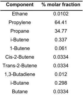
The propylene splitter studied here is part of an industrial propylene production unit from the Petrobras Capuava Refinery (RECAP) located at Mauá, São Paulo, Brazil. This process was designed to produce 145 000 ton/year of propylene polymer grade with high purity (99.5% molar at least). This production unit consists of three distillation columns: depropanizer, deethanizer and depropenizer. The bottom liquid product from the deethanizer (T-02) is mixed with similar composition streams (Propint) of other refineries to feed the propylene/propane splitter (T-03). That is the reason for using the feed flow-rate as a manipulated variable in the advanced control strategy as it will be shown in subsection 3.4.2. The propylene/propane splitter operates at a pressure of 9 kgf/cm2 (gauge) and is equipped with 157 valve trays. In this section, which is schematically represented in Fig. 3.1, propylene is separated from propane which also carries other hydrocarbons with four atoms of carbon. A typical feed composition of column T-03 is shown in Table 3.1. The propylene stream is produced as the top stream of the splitter and is sold to a nearby petrochemical plant, and the propane stream obtained as the bottom product is stored in propane spheres and sold as liquefied petroleum gas (LPG).
Table 3. 1 – Typical feed composition of propylene/propane splitter
Component % molar fraction
Ethane 0.0102
Propylene 64.41
Propane 34.77
i-Butene 0.337
1-Butene 0.061
Cis-2-Butene 0.0334
Trans-2-Butene 0.0334
1,3-Butadiene 0.012
i-Butane 0.298
The distillation system studied here includes an energy recovery system through the use of heat integration. As it can be observed from Fig. 3.1, there is a vapor recompression system, which has become the standard heat pump technology in distillation systems. Energy savings of about 50% have been reported in high-purity separation processes (Bruinsma and Spoelstra, 2010). In this way, compressor V-01 increases the pressure and temperature of the vapor leaving the top of the column to about 7 kgf/cm2 and 30°C, and this recompressed vapor is condensed in the reboilers M-01 A/B and M-02 at the bottom section of the column. This column presents three bottom reboilers that work in parallel. Reboilers M-01 A/B are vertical, while reboiler M-02, which was included in a revamp project of the system, is horizontal. All of them present variable exposed heat transfer area that depends on the condensed liquid level in drums O-03 and O-04.
The top column product is sent to the compressor suction drum (O-01) and after that, the vapor phase stream is compressed in the propylene compressor (V-01). It increases the pressure until 16.2 kgf/cm2 and the temperature approximately up to 50°C in order to allow the exchange of heat in the column reboilers (01A/B and M-02). This process stream is divided in three different streams, one of them goes to the M-01A/B reboilers and is collected in the drum O-03. After that, it is cooled to 35 °C in the water cooler M-04; the second stream goes to reboiler M-02 and is collected in the drum O-04, and the last stream goes to the water cooler M-03A/B so that column’s top pressure could be controlled.
The outlet liquid products of M-04, M-02 and M-03A/B are mixed together and sent to the reflux separator (O-02). The O-02 liquid product is divided into two streams, one of them is sent back to the column as a reflux, and the other stream is the propylene product that is pumped to the customer storage spheres.
3.2 Equipment description
In this section, the main equipments of the Propylene/Propane splitter are described for a better understanding of the process and process operating conditions.
3.2.1 Depropenizer splitter (T-03)
This column, where the separation between propylene and propane is carried out, contains 157 trays. The high number of trays is typical in this type of process because of the difficult separation between propylene and propane and the desired high purity of the propylene product. Some of the process conditions of this column are describe in Table 3.2.
Table 3. 2 – Column T-03 description
Description Value Unit of
measurement Top operation pressure 9 kgf/cm2 g
Top operation temperature 18.9 °C
Bottom operation temperature 28.9 °C
3.2.2 Propylene compressor (V-01)
This compressor is the heart of the energy integration system used in this process. It increases the pressure up to 16.2 kgf/cm2 where the propylene temperature is, approximately, 50.4 °C. This compressed stream is cooled in the bottom column reboilers and in the water cooler M-03 A/B. The compressor runs at a fixed rotation speed of 7250 rpm.
3.2.3 Heat exchangers
In this process unit, there are four heat exchangers that are described below, some of them are used as reboilers and others as water coolers.
3.2.3.1 Reboilers M-01 A/B
These heat exchangers are the reboilers of the T-03 splitter. The heat transferred from the compressed propylene to the bottom liquid product (propane) enables the vaporization of propylene, therefore, minimizing the loss of propylene in the bottom stream. These reboilers are vertical and connected in parallel. The required information about these reboilers is described in Table 3.3:
Table 3. 3 – Heat exchangers M-01 A/B description
Description Value
Number of passes 1
Orientation Vertical Number of tubes 6829
Outside tube
diameter 15.9 mm
Tube length 6096 mm
Shell side Tube side
Product Propylene Propane Inlet temperature 50.4 °C 28.9 °C Outlet temperature 39.3 °C 29.3°C
3.2.3.2 Reboiler M-02
same purpose as reboilers M-01 A/B, but it has difference characteristics as shown in Table 3.4:
Table 3. 4 – Heat exchanger M-02 description
Description Value
Number of passes 2
Orientation Horizontal Number of tubes 1978
Outside tube
diameter 15.87 mm
Tube length 6000 mm
Shell side Tube side
Product Propane Propylene Inlet temperature 28.9 °C 50.4 °C Outlet temperature 29.3 °C 39.3 °C
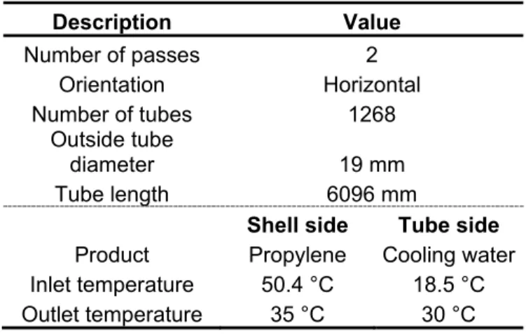
3.2.3.3 Cooler M-03 A/B
These water coolers are connected in parallel and cool the compressed propylene stream in order to allow the control of the column pressure at 9.0kgf/cm2. The temperature is decreased down to 35 °C and after that it goes to the reflux separator O-02. One of these equipments has the description given in Table 3.5:
Table 3. 5 – Heat exchangers M-03 A/B description
Description Value
Number of passes 2
Orientation Horizontal Number of tubes 1268
Outside tube
diameter 19 mm
Tube length 6096 mm
Shell side Tube side
Product Propylene Cooling water Inlet temperature 50.4 °C 18.5 °C Outlet temperature 35 °C 30 °C 3.2.3.4 Cooler M-04
Table 3. 6 – Heat exchanger M-04 description
Description Value
Number of passes 2
Orientation Horizontal Number of tubes 1050
Outside tube
diameter 19 mm
Tube length 6096 mm
Shell side Tube side
Product Propylene Cooling water Inlet temperature 39.3 °C 18.5 °C Outlet temperature 35 °C 30 °C
3.2.4 Drums and separators
The propylene/propane separation system has a number of auxiliary drums and separators that need to be included in the dynamic simulation of the system.
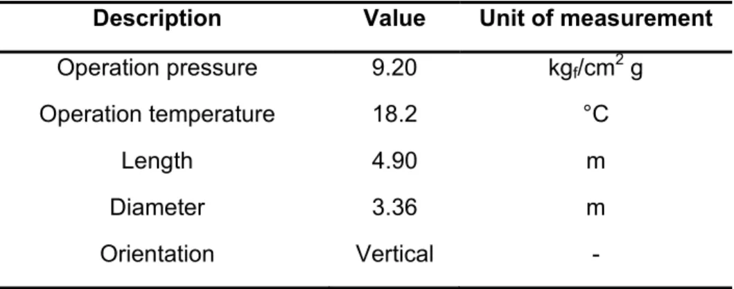
3.2.4.1 Drum O-01
This is the suction drum of compressor V-01, which is also fed with the vapor phase stream of O-02. Its main objective is to avoid that any liquid to be carried to the compressor, because it would damage the compressor. The process conditions and dimension of this drum are given in Table 3.7.
Table 3. 7 – Drum O-01 description
Description Value Unit of measurement Operation pressure 9.20 kgf/cm2 g
Operation temperature 18.2 °C
Length 4.90 m
Diameter 3.36 m
Orientation Vertical -
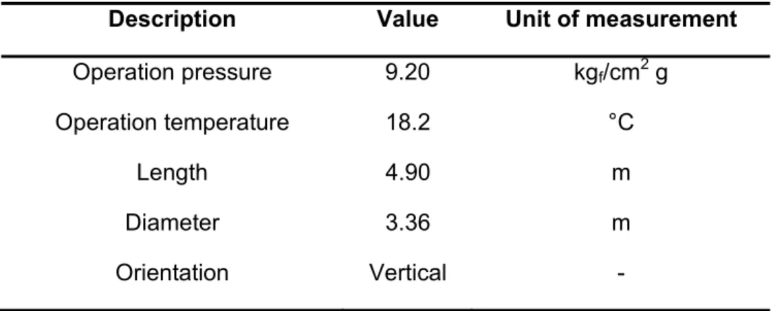
3.2.4.2 Separator O-02
there is a partial vaporization of the liquid stream and some vapor is generated and sent to the compressor suction drum O-01. The outlet liquid stream of this separator is divided in two, one returns to the column as the reflux and the other goes to the propylene storage sphere. The conditions and dimension of this drum are given in Table 3.8.
Table 3. 8 – Separator O-02 description
Description Value Unit of measurement
Operation pressure 9.20 kgf/cm2 g
Operation temperature 18.2 °C
Length 4.90 m
Diameter 3.36 m
Orientation Vertical -
3.2.4.3 Drum O-03
This drum is located below reboilers M-01 A/B, in order to establish a liquid level that modifies the heat transfer area of these reboilers. Then, its main objective is to allow a reduction or increase of the reboiler’s heat exchange area. The details about this drum are given in Table 3.9.
Table 3. 9 – Drum O-03 description
Description Value Unit of measurement
Operation pressure 15.8 kgf/cm2 g
Operation temperature 39.3 °C
Length 1.70 m
Diameter 0.85 m
3.2.4.4 Drum O-04
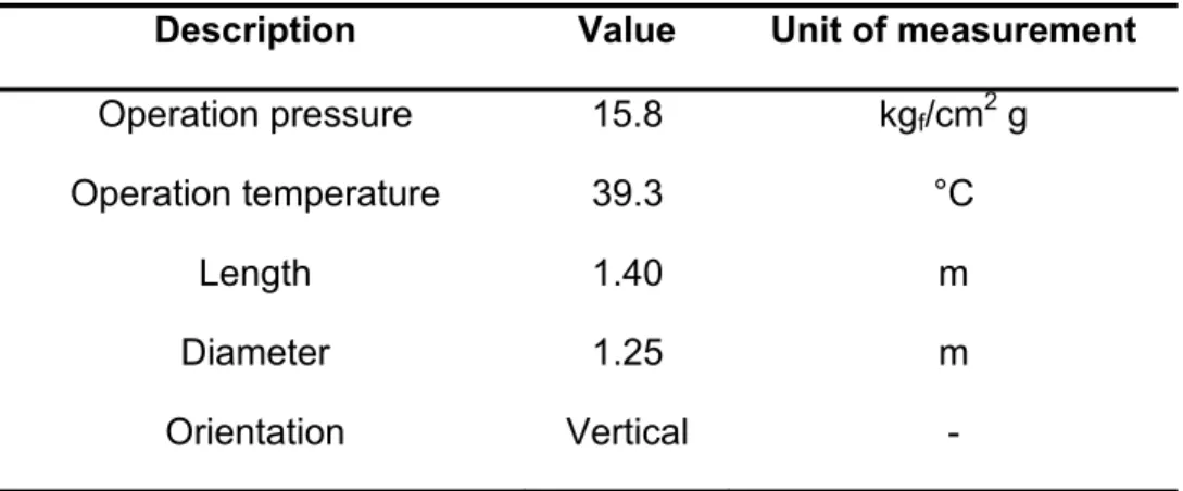
This drum is located below reboiler M-02 in order to establish a liquid level that modifies the heat transfer area of the reboiler. The required details for the simulation of this drum are given in Table 3.10.
Table 3. 10 – Drum O-04 description
Description Value Unit of measurement
Operation pressure 15.8 kgf/cm2 g
Operation temperature 39.3 °C
Length 1.40 m
Diameter 1.25 m
Orientation Vertical -
3.3 Existing multivariable advanced controller (LDMC)
In order to maintain the propylene product specification and to minimize the loss of propylene to the propane product stream, it has been already implemented a conventional advanced controller of the DMC type (LDMC - Linear Dynamic Matrix Controller). This controller is based on the step response coefficients of the plant and, although it has shown a good performance from the viewpoint of keeping the controlled variables inside their control zones, it does not have a guarantee of stability and it is not integrated with a RTO algorithm. The existing controller considers a control structure where there are three manipulated variables to control another three outputs. The control structure is described in the next section.
3.3.1 Controlled variables (Outputs)
The existing advanced control structure aims at the control of the following variables:
Liquid level on heat exchangers M-01 A/B and O-03 (LC-5)
liquid level of 80%, the heat transfer area corresponds to only 20% of the total area. The total height considered for the level controller (LC-5) is the sum of the reboiler height and drum O-03 height, because the reboiler is exactly above drum O-03. This controlled variable is used to guarantee a minimum level for pumping and a maximum liquid level for process safety.
Propane molar composition in the propylene stream (AC-1)
This controlled variable (y2) indicates the quality of the propylene product that must have a molar composition of at least 99.5%. This means that the molar percentage of propane in the propylene stream must have a maximum value of 0.5%, which is measured through a composition analyzer.
Propylene molar composition in the propane stream (AC-2)
This controlled variable (y3) corresponds to the amount of propylene that is lost to the propane stream. In the conventional advanced control structure, this loss of propylene is limited to an upper bound of 8% of propylene in the propane stream, but it should be limited to an upper bound of about 2% for an optimal operation of the process.
3.3.2 Manipulated variables (Inputs)
The existing controller manipulates the following variables in order to maintain the controlled variables defined in the previous section inside their respective control zones.
Heat pump flow rate set-point (FC-3)
Feed flow rate set-point (FC-1)
This process variable set-point (u2) affects the three controlled outputs and can be manipulated in order to maintain all the controlled variables inside their respective control zones. However, this variable should be mainly manipulated to maximize the propylene production and to achieve the scheduled propylene production.
Reflux flow rate set-point (FC-2)
The reflux flow rate set-point (u3) is manipulated mainly to attain the high purity of the propylene product stream. It has a strong influence on that controlled variable. The controller tends to manipulate the column reflux to obtain a product of at least 99.5% molar of propylene.
3.4 Dynamic simulation of the PP Splitter
The dynamic simulation of the propylene distillation column was developed using the software SimSci Dynsim. The idea is to consider the rigorous dynamic model as the virtual plant so that the advanced control implementation, controller tuning and model identification will be developed and tested without any cost (Dynsim User Guide, 2012). In order to represent a realistic operating scenario, all the regulatory PID control loops will be included in the simulation besides the advanced control and real time optimization algorithms. This dynamic simulation will also be useful to identify the linear dynamic models at different operating points, which will be used in the IHMPC and RIHMPC.
3.4.1 Equipment description for the dynamic simulation
3.4.2 Valve coefficients
The valve coefficients (Cv) of the main control valves of the system must be provided so that the dynamic simulation can be built up.
Table 3. 11 – Valve coefficients (Cv)
Valve Tag Cv
FV-1 47
FV-2 780
FV-3 500
FV-4 46
FV-5 26
FV-6 80
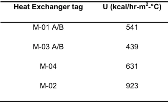
3.4.3 Heat transfer coefficients
The heat transfer coefficients of the four heat exchangers of the Propylene/propane system are shown in Table 3.12.
Table 3. 12 – Overall heat transfer coefficients
Heat Exchanger tag U (kcal/hr-m2-°C)
M-01 A/B 541
M-03 A/B 439
M-04 631
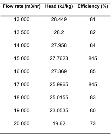
3.4.4 Curve of theheat pump compressor Table 3. 13 – Compressor V-01 curves
Flow rate (m3/hr) Head (kJ/kg) Efficiency (%)
13 000 28.449 81
13 500 28.2 82
14 000 27.958 84
15 000 27.7623 845
16 000 27.369 85
17 000 25.9965 845
18 000 25.0155 83
19 000 23.0535 80
20 000 19.62 73
3.4.5 Main dimensions of the Propylene/Propane splitter
Table 3. 14 – Dynamic equipment data T-03
Description Value Units Tray spacing 0.45 m
Sump diameter 4.2 m
Sump height 2.55 m
Column diameter 4.2 m
3.4.6 Regulatory level PID control loop strategies and tuning Table 3. 15 – Main PID controllers used in the propylene/propane splitter
PID controller Function
FC-1 Feed flow rate to column T-03
PC-1 Pressure at the top of T-03
LC-1 Liquid level at the bottom of T-03
FC-2 Reflux flow rate to column T-03
PC-2 Pressure at the outlet of compressor V-01 (Relief)
LC-2 Liquid level in the knockout drum O-01
FC-3 Total vapor flow rate through the heat pump
LC-3 Upper-liquid level in separator O-02
LC-3A Lower-liquid level in separator O-02
FC-4 Propylene flow rate to storage
LC-4 Liquid level in drum O-04 and reboiler M-02
FC-5 Propane flow rate to storage
LC-5 Liquid level in drum O-03 and reboilers M-01 A/B
FC-6 Flow rate through water cooler M-03
FC-7 Outlet flow rate of drum O-04
AC-1 Propane molar composition in the propylene product stream
AC-2 Propylene molar composition in the propane product stream
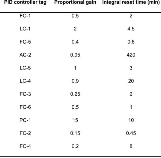
way, LC-4 and FC-7 are cascaded such that the liquid level in drum O-04 is kept at 65%. Also, PC-1 and FC-6 are cascaded such that FC-6 set-point is manipulated to keep the column top pressure at 9.0 kgf/cm2. There is an override control strategy involving controllers LC-3, LC-3A and FC-4. The resulting signal of the high selector between LC-3 and FC-4 is sent to a low selector between this signal and the output of LC-3A so that propylene liquid level in separator O-02 is held between its upper and lower limits. As the propylene product purity is important, there is a composition analyzer (AC-1) that cascades FC-2 so that reflux flow rate set-point changes depending of the AC-1 output. Finally, in order to minimize the loss of propylene to the bottom product of T-03, there is a composition analyzer (AC-2) that cascades FC-3, the resulting signal is sent to a low selector with LC-5 output so that a minimum liquid level in drum O-03 will be maintained. The tuning parameters of the PID controllers are summarized in Table 3.16.
Table 3. 16 – Main PID controller tuning
PID controller tag Proportional gain Integral reset time (min)
FC-1 0.5 2
LC-1 2 4.5
FC-5 0.4 0.6
AC-2 0.05 420
LC-5 1 3
LC-4 0.9 20
FC-3 0.25 2
FC-6 0.5 1
PC-1 15 10
FC-2 0.15 0.45
PID controller tag Proportional gain Integral reset time (min)
LC-2 2 1
LC-3 1.5 2
LC-3A 1 0.5
PC-2 20 10
FC-7 0.6 1
AC-1 0.08 360
3.4.7 Initialization and convergence
The initialization or convergence to an initial steady-state of the dynamic simulation of the PP splitter is difficult and complex because most of the PID regulatory would be in manual mode and process operation knowledge is needed to stabilize the process system. In Dynsim, there are algorithms for the initialization at a converged known steady-state. Initially, it is necessary to estimate the composition and flow rates of the top and bottom products. Then, the operation of the plant should be simulated with the PID regulatory controllers in manual mode until the pressure of the column and the liquid levels inside the vessels are near the normal operation values. Then, PID controllers can be switched on to the automatic mode.
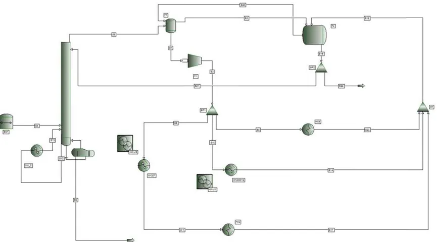
3.4.8 The in Dy
8
complete ynsim is sh
Figure 3.
PFD of process flo hown in Fig
. 2 – Snapsh
the propy ow-sheet d gure 3.3.
hot summary
ylene/prop diagram (P
of the PP Sp
pane splitt PFD) of the
plitter in Dyn
terin Dyns PP splitte
nsim
sim
4 D In th robu imple 4.1 The to ob resp perfo the i The to se the m wou syste DEVELOP his chapter ust advanc emented in
Mo first stage btain the p ponse mod
ormed with nputs with
results of ee that ea model iden ld be expe em (about
Figure 4
PMENT OF
r, the steps ced contro
n the propy
odel identif in the imp process m
el. Consid h the rigoro
sizes in th
these exp ach operati ntification ensive and
30h).
. 1 – Selecte
F THE PRO
s that wer llers are d ylene splitt
fication plementatio
odel, in th ering the l ous dynam he range o
periments a ing point c
experimen very time ed manipulat OPOSED A re followed described. ter and inte
on of any a is case, a ayout of th mic simulat f 1 – 5% o
are summa correspond nts were p
consuming
ed and contr
ADVANCE
d in the de These co egrated wit
advanced c linear dyn he process
tion consid of the full in
arized in F ds to a diff performed
g because
rolled variabl
ED CONTR
velopment ntrollers w th the real
control bas namic mod s in Figure dering step nput range
Figure 4.2, ferent step
in the rea e of the hig
le for the ste
ROL STRA
t of the no were propo time optim
sed on line del such a 4.1, step t p in the se of each in
where it i p response
l industrial h settling t
ep response t
ATEGY
ominal and osed to be mization.
ear MPC is s the step tests were et-points of
put.
s possible e model. If l system it time of the
y1 y2 y3 The follow cond capa capa proc Pro Feed T Fig
three diff wing oper dition; Poin acity; Poin acity as de cess history
ocess varia
d flow rate Top column
pressure u1
ure 4. 2 – St
ferent ope ating cond nt 1 corres nt 2 corres efined in Ta
y database
Table 4
able
(u2) T
n kg
tep response
erating po ditions: Po sponds to sponds to able 4.1. T e of the las
. 1 – Differen
UOM
Ton./h
gf/cm2g
u2
es of the PP
ints prese int 3 corre an operat an operat These oper st two year
nt operating c
Operat Point
29.51
9.0
2
splitter at dif
ented in F esponds to ting condit
ting point rating poin rs. conditions of ing 1 1 fferent opera
Figure 4.2 o the most
ion with a with an in ts were se
f the PP split
Operating Point 2 32.3 9.0 u3 ting points correspo t common
reduced p ncreased p elected bas
tter
g Op
P
nd to the operating production production sed on the
Process variable UOM Operating Point 1 Operating Point 2 Operating Point 3
Reflux flow rate
(u3) Ton./h 255.8 273.02 268.0
Reflux
temperature °C 18.9 18.99 19.5
Compressor outlet
temperature °C 50.4 48.9 50.01
Reboiler M-01 A/B
liquid level (y1) % 51.9 49.6 42.1
Total heat pump
flow rate (u1) Ton./h 281.28 289.13 302.0
Propylene product
flow rate Ton./h 17.79 19.48 18.45
Propane molar composition in Propylene stream
(y2)
% 0.35 0.436 0.5
Propane product
flow rate Ton./h 11.72 12.82 11.55
Propylene molar composition in Propane stream
(y3)
% 8.0 7.54 1.0
So, in the proposed robust controller, the dynamics of the non-linear distillation system will be approximately represented through three linear models that constitute the multi-model set on which the robust controller will be based. The third model will be used to implement the nominal IHMPC, which is based on the nominal model.