Experiments in Globalisation, Food
Security and Land Use Decision Making
Calum Brown1*, Dave Murray-Rust1¤, Jasper van Vliet2, Shah Jamal Alam1, Peter H. Verburg2, Mark D. Rounsevell1
1.School of GeoSciences, University of Edinburgh, Edinburgh, EH8 9XP, United Kingdom,2.Institute for Environmental Studies, VU University Amsterdam, Amsterdam, The Netherlands
¤ Current address: School of Informatics, University of Edinburgh, Appleton Tower, 11 Crichton Street, Edinburgh, EH8 9LE, United Kingdom
Abstract
The globalisation of trade affects land use, food production and environments around the world. In principle, globalisation can maximise productivity and
efficiency if competition prompts specialisation on the basis of productive capacity. In reality, however, such specialisation is often constrained by practical or political barriers, including those intended to ensure national or regional food security. These are likely to produce globally sub-optimal distributions of land uses. Both outcomes are subject to the responses of individual land managers to economic and environmental stimuli, and these responses are known to be variable and often (economically) irrational. We investigate the consequences of stylised food security policies and globalisation of agricultural markets on land use patterns under a variety of modelled forms of land manager behaviour, including variation in production levels, tenacity, land use intensity and multi-functionality. We find that a system entirely dedicated to regional food security is inferior to an entirely
globalised system in terms of overall production levels, but that several forms of behaviour limit the difference between the two, and that variations in land use intensity and functionality can substantially increase the provision of food and other ecosystem services in both cases. We also find emergent behaviour that results in the abandonment of productive land, the slowing of rates of land use change and the fragmentation or, conversely, concentration of land uses following changes in demand levels.
OPEN ACCESS
Citation:Brown C, Murray-Rust D, van Vliet J, Alam SJ, Verburg PH, et al. (2014) Experiments in Globalisation, Food Security and Land Use Decision Making. PLoS ONE 9(12): e114213. doi:10.1371/journal.pone.0114213
Editor:Tobias Preis, University of Warwick, United Kingdom
Received:July 14, 2014
Accepted:October 31, 2014
Published:December 1, 2014
Copyright:ß2014 Brown et al. This is an open-access article distributed under the terms of theCreative Commons Attribution License, which permits unrestricted use, distribution, and reproduction in any medium, provided the original author and source are credited.
Data Availability:The authors confirm that all data underlying the findings are fully available without restriction. The model used in this study is freely available online via https://www.wiki.ed.ac.uk/ display/CRAFTY/Home. Model setup is described in the manuscript and Supporting Information, and all data are available athttp://datashare.is.ed.ac.uk/ handle/10283/644.
Funding:This work was carried out as part of the Visions of Land Use Transitions in Europe (VOLANTE) project (http://www.volante-project.eu/), funded by the European Commission under the Environment (including climate change) Theme of the 7th Framework Programme for Research and Technological Development: Volante -FP7-ENV-2010-265104. The funders had no role in study design, data collection and analysis, decision to publish, or preparation of the manuscript.
Introduction
In neoclassical economic theory, globalisation underpinned by free trade will produce an optimal distribution of land uses, so that goods and services are produced wherever it is most efficient – and cheapest – to do so, providing benefits throughout the supply chain [1,2]. This implies separation of sites of production and consumption of goods and services, with major consequences for existing patterns of agricultural land uses in particular [3]. While some
governments and international bodies promote trade of this kind (e.g. [4–6]), it is more commonly opposed in the interests of national or regional food security, to balance the interests of productive and economically important industries, conserve biodiversity, or respect public demand for various land uses [7–9].
Policies that aim to ensure food security notably include the European Union’s Common Agricultural Policy (CAP). Intended to maintain a level of self-sufficiency in Europe, the CAP provides support for European agriculture at the expense of potentially more efficient production elsewhere in the world [10]. If production levels and land use efficiency are maximised by global free trade amongst purely rational agents (who are in full possession of relevant knowledge and account for environmental externalities), directed interventions of this kind lead only to sub-optimal outcomes by reducing and slowing the global influence on local land use change. Resulting land use configurations are, in theory, less efficient, productive and profitable than those arising from unfettered trade in agricultural goods. In the case of the CAP, regional overproduction of food and environmentally damaging intensification of agriculture has been stimulated at times, alongside land abandonment in marginal areas (e.g. [11,12]).
Behavioural effects are likely to be especially strong in a changing system. For example, land managers who differ in their ability or willingness to meet demands for particular services are likely to show strongly divergent responses to changing demand levels [22], while those who are most dependent upon natural resources need to be most adaptable to climate change [23]. In theory, globalised systems are adept at coping with such changes in demand or contextual factors, allowing compensatory adjustments to spread quickly following a disturbance somewhere in the system [24]. However, the behaviour of individual land managers has the potential to undermine this process, and so the true implications of global and regional approaches to food security under climatic and societal change remain uncertain.
Despite the importance of these issues, the effects of land managers’ responses to change in globalised and regionalised land systems have not been fully investigated beyond analysis with macro-level models based only on economic theory [2]. Methods do exist to investigate these effects, and foremost among these are Agent-Based Models (ABMs) that attempt to describe the effects of individual behaviours on complex systems [25–28]. Nevertheless, to our
knowledge, ABMs have not been used to investigate, systematically, responses to policies dedicated to maximising global food production or ensuring regional food security in dynamic land use systems.
Here we use a set of simulation experiments with a land use ABM to examine the effects of land managers’ individual behaviours on the configurations, productivities, and efficiencies of land uses in idealised global and regional land use systems (in which globalisation and regionalisation occur perfectly, with either completely free or completely limited trade in goods and services). Specifically, we investigate the role of land manager behaviour that is not strictly ‘rational’ in driving deviations from optimal land use configurations (i.e., configurations where production per unit area is maximised), the potential consequences of this for food security in globalised and regionalised systems, and the effects of multi-functional land use on the production of food and other ecosystem services.
Methods
1. Overview of model
Agents are characterised according to the Agent Functional Type concept [26,30], which suggests that land managers may be grouped by behaviour or by their productive response to environmental (locational) conditions, in analogy to plant functional types (PFTs) in ecosystem models. Each AFT has a different production function, describing its ability to utilise particular capitals in order to produce particular ES, and may also have additional distinct behavioural settings. Within each type, agents may be homogeneous or heterogeneous.
A fundamental basis for agent behaviour in the model is provided by
abandonment and competition thresholds that describe agents’ willingness to abandon or relinquish land. Agents in the model compete for available land parcels (represented by cells in a grid) based on these two parameters. The inspiration for this simple behavioural representation comes from several studies that have suggested that a wide range of behaviours are reducible to a small number of dimensions of this kind (e.g. [16,31]). We use these thresholds to represent real-world variation in personal characteristics or decision-making strategies that alter land managers’ dedication to their land use, and they can be used in this way to encapsulate variation in culture, profit-sensitivity, available labour pool, personal financial resources and other similar factors as appropriate. They can also be used to account for costs of production or change of land use, when a minimum return is required to avoid a net loss being made. Also included are parameters that control an agent’s ability to search for suitable cells and those describing an agent’s production function.
Once parameterised, the model runs through a series of ‘timesteps’, each of which typically represents a single year. At each timestep, searches are undertaken by a typical agent of each type, in order to identify cells where their productive ability is maximised. Both the number of searches carried out and the number of cells considered during each search are specified (Table 1). Searched cells are ranked after each search according to the competitiveness of that AFT at that location, and individual agents then attempt to take over these cells, in order, until one cell is taken over or the list of cells is exhausted. Competitiveness is calculated on the basis of an AFT’s mean (or uniform) ES production, which is given a utility value via a function linking unmet demand and production levels.
Agents continue production as long as their utility value is greater than their abandonment threshold (the value representing the lower limit at which an agent can or will persist with a land use), and will only relinquish land to a competitor with a utility that exceeds their own by more than their competition threshold. Agents therefore succeed in taking over a cell when that cell is currently
2. Experimental setup
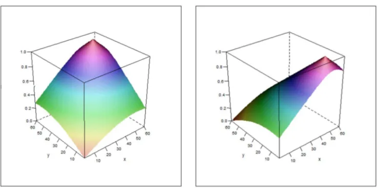
Our experiments are designed to investigate effects of land manager behaviour on land use under globalisation and regionalisation of demand for food and other ecosystem services. We start with a simple baseline model intended to investigate the effects of regionalisation and changing demand levels in the absence of any confounding processes. We then add complexity to this model as detailed below. Throughout, we use the same modelled world (or arena), represented by a 60 by 60 cell grid, with two distinct capitals (crop productivity and natural capital) that vary across the grid. Under regionalisation, this grid is divided into four 30 by 30 cell regions. The maximum values of both capitals are located on the same side of the arena (Fig. 1) to generate competition between agents for highly productive areas.
Each cell in the world may be managed by a single agent, and agents are distributed across the world randomly at the start of each simulation. The agents then compete for land over the course of 25 timesteps. We run 30 realisations of each experimental setup in order to construct envelopes of results that provide information about the relative strength of stochastic and systematic variation within and between simulations. We also monitor the time taken for
productivities to converge to a steady state across realisations of each experiment, both from the initial agent distribution and following a change in demand levels (with a steady state defined as the state where the annual variation in ES supply between realisations is greater than the difference between annual mean ES supplies across realisations). The rationale and parameter settings for each simulation are given in Tables 2and 3.
3. Simulation schedule
Our baseline simulation is one in which two agent functional types (AFTs) – ‘farmers’ and ‘conservationists’ – compete to satisfy abstract demands for food and recreation. The identities of these AFTs are arbitrary and are used to differentiate the two rather than to link them to real-world characteristics of such land managers. Farmer productivity depends on the crop productivity capital and
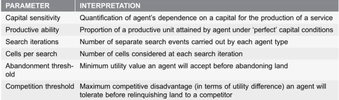
Table 1.Descriptions of the main parameters in the model. PARAMETER INTERPRETATION
Capital sensitivity Quantification of agent’s dependence on a capital for the production of a service Productive ability Proportion of a productive unit attained by agent under ‘perfect’ capital conditions Search iterations Number of separate search events carried out by each agent type
Cells per search Number of cells considered at each search iteration Abandonment
thresh-old
Minimum utility value an agent will accept before abandoning land
Competition threshold Maximum competitive disadvantage (in terms of utility difference) an agent will tolerate before relinquishing land to a competitor
conservationist productivity depends on the natural amenity capital. Both AFTs are capable of producing a single ‘unit’ of their ES under optimum conditions (where the relevant capital is maximised, at a value of 1) (Table 4).
Figure 1. Variation in productivity capitals across the modelled arena.Crop productivity is shown on the left and natural capital on the right. Both are maximised on the right-hand-side of the arena in order to allow separation of agent types while generating competition for the most productive cells. doi:10.1371/journal.pone.0114213.g001
Table 2.Descriptions and rationales for the experiments.
EXPERIMENT(S) DESCRIPTION RATIONALE
1 Baseline experiment To establish land use configurations in the absence of any behaviour.
2–5 Variations in abandonment thresholds To investigate effects of raised abandonment thresholds (unwillingness to accept low returns) in either (2–3) or both (4) agent types, and when individual variation occurs (5). 6 Variation in competition thresholds To investigate effects of raised competition thresholds
(unwill-ingness to relinquish land), with individual variation.
7 Reduced ability to search for cells To establish effects of a reduction in agents’ ability to search for cells on which to compete.
8 Decreased sensitivity to demand levels (exponential form of utility functions to give positive utility in the case of over-supply of services)
To investigate effects of (a) insensitivity to demand levels, or (b) personal motivation for production, or (c) a cross-regional market giving value to overproduction.
9–13 Variable intensities of land use with and without additional behaviour as above
To investigate how above effects change when different intensities of land uses are available.
14–19 Multifunctional and variable intensity land uses with and without additional behaviour as above.
To investigate how land use multi-functionality changes the above effects under different behaviours.
Initially, utility for both services is represented by a linear functiony5ax, where y is the utility for the production of a unit of an ES, andxis the unmet demand for this ES. A linear function is chosen for its generality and interpretability, with
Table 3.Parameter settings used in the experiments.
EXPERIMENT HIF MIF LIF CONS SEARCH CELLS/SEARCH
UTILITY FUNCTION AT; CT AT; CT AT; CT AT; CT ITS.
1 0.0; 0.0 NA NA 0.0; 0.0 5000 10 y53x
2 0.2; 0.0 NA NA 0.0; 0.0 5000 10 y53x
3 0.0; 0.0 NA NA 0.2; 0.0 5000 10 y53x
4 0.2; 0.0 NA NA 0.2; 0.0 5000 10 y53x
5 0.0; 0.0 NA NA N(0.2,0.03); 0.0 5000 10 y53x
6 0.0; 0.0 NA NA 0.0;N(0.2,0.03) 5000 10 y53x
7 0.0; 0.0 NA NA 0.0; 0.0 100 10 y53x
8 0.0; 0.0 NA NA 0.0; 0.0 5000 10 y5ex
9 0.0; 0.0 0.0; 0.0 0.0; 0.0 0.0; 0.0 5000 10 y53x
10 0.2; 0.0 0.0; 0.0 0.0; 0.0 0.2; 0.0 5000 10 y53x
11 0.0; 0.0 0.0; 0.1 0.0; 0.2 0.0; 0.0 5000 10 y53x
12 0.0; 0.0 0.0; 0.0 0.0; 0.0 0.0; 0.0 5000 10 y5ex
13 0.0; 0.0 0.0; 0.1 0.0; 0.2 0.0; 0.0 5000 10 y5ex
14 0.0; 0.0 0.0; 0.0 (Multi) 0.0; 0.0 (Multi) 0.0; 0.0 5000 10 y53x
15 0.2; 0.0 0.0; 0.0 (Multi) 0.0; 0.0 (Multi) 0.2; 0.0 5000 10 y53x
16 N(0.2,0.03); 0.0 0.0; 0.0 (Multi) 0.0; 0.0 (Multi) N(0.2,0.03); 0.0 5000 10 y53x
17 0.0; 0.0 N(0.2,0.03); 0.0 (Multi)
N(0.2,0.03); 0.0 (Multi)
0.0; 0.0 5000 10 y53x
18 0.0; 0.0 0.0; 0.1; Multi 0.0; 0.2; Multi 0.0; 0.0 5000 10 y53x
19 0.0; 0.0 0.0; 0.0 (Multi) 0.0; 0.0; (Multi) 0.0; 0.0 5000 10 y5ex
Settings that are altered relative to Experiment 1 in each case are in bold. Each Experiment is run four times (labelled asa,b, c,d); once for each combination of static and dynamic demand with globalised and regionalised configurations (a5static globalised, b5dynamic globalised, c5static
regionalised, d5dynamic regionalised). N(y,z) denotes a Gaussian distribution with meanyand standard deviationz. Agent types are denoted as follows:
HIF5high-intensity farmers; MIF5mid-intensity farmers; LIF5low-intensity farmers; Cons5conservationists. AT and CT refer to Abandonment
Thresholds and Competition Thresholds, respectively. doi:10.1371/journal.pone.0114213.t003
Table 4.Capital sensitivities and production levels for each agent type used in the experiments.
AGENT TYPE
SENSITIVITY TO CROP PRODUCTIVITY
SENSITIVITY TO
NATURAL CAPITAL FOOD PRODUCTION
RECREATION PRODUCTION
High Intensity Farmer 1.0 0.0 1.0 0.0
Mid Intensity Farmer (1) 0.5 0.0 0.5 0.0
Low Intensity Farmer (1) 0.25 0.0 0.25 0.0
Mid Intensity Farmer (2) 0.75 0.20 0.75 0.15
Low Intensity Farmer (2) 0.35 0.4 0.35 0.4
Conservationist 0.0 1.0 0.0 1.0
increasing levels of unmet demand generating steady increases in utility values. Negative values are set to zero, so that overproduction of an ES is neither to the benefit nor detriment of an agent (the value of the gradient a in this linear relationship is arbitrary and set here to 3.0 for both services; changes in this value would alter the rate at which responses to changes in demand levels occurred, but not the relative competitiveness of modelled service production). Abandonment and competition thresholds are initially set to 0.0, so that agents relinquish land when they do not have a positive competitiveness or when another agent has a higher competitiveness. At each timestep, each AFT undertakes 5,000 search iterations of 10 randomly-selected cells and then attempts to take over these cells.
Demand levels are set so that an optimum agent configuration is almost capable of satisfying global demands for food and recreation, which are equal and static (so that every cell is required for production and is subject to competition between agents). In order to investigate the effects of dynamic demand we then introduce a step-change in demand during the relevant simulations, with demand for recreation dropping by 75% after 11 timesteps. Subsequently, these same static and dynamic demands are divided between four equally-sized regions in order to investigate the effects of regionalisation caused by policies dedicated to regional food security. Beyond this, we include no political or economic barriers to the establishment of optimal land use patterns (policies that slow or prevent large-scale land use change are not simulated, for instance), so that the effects of modelled behaviour can be isolated.
4. Behavioural variations
Using the above basic settings, we vary model parameters to introduce individual and typological agent behaviour, and to relax the distinction between regionalised and globalised systems. We first vary abandonment thresholds, systematically and stochastically, for both AFTs. We then similarly vary competition thresholds, before altering agents’ abilities to search and compete for cells, and changing the form of the utility functions. The parameter values used in each case and rationales for these changes are given in Tables 2 and 3.
Following these behavioural variations, we introduce two additional AFTs – mid-and low-intensity farmers - to the simulations. At first, these types produce only food, and are distinguished from high-intensity farmers by their reduced sensitivity to capital levels and their reduced productive ability. Later, we allow these agents to adopt multi-functional land uses, so that, in addition to food, they also produce recreation while having limited sensitivity to the relevant capitals (Table 4). In both cases, we introduce some of the above behavioural variations, which we do not attempt to link to particular human behaviours or characteristics, because the nature, number and complexity of these factors effectively preclude the
identification of such links (e.g. [26,32]). Instead, we use systematic and stochastic variation between and within AFTs to identify the general effect of broad
this kind [16,33]. We discuss links between our simulated variations and real-world land manager behaviour inTables 2and5, and in the Discussion section.
Results
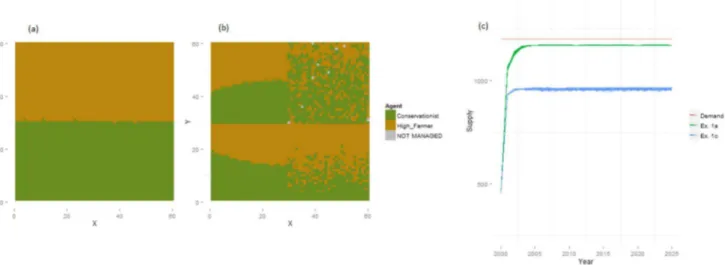
A full description of the results is given here, while principal findings are summarised in the Discussion section below, and in Table 5. The basic model setup (Experiment 1) was used to explore the effects of globalised and regionalised demand in the absence of any behaviour, providing a baseline for further experiments. Agents in the static globalised system quickly converged to a near-optimal configuration (Table S1 in file S1) in which each type occupied areas where it was particularly productive (Fig. 2a;Table 4). This allowed supply levels for food and recreation to remain stable and equal, nearly meeting global
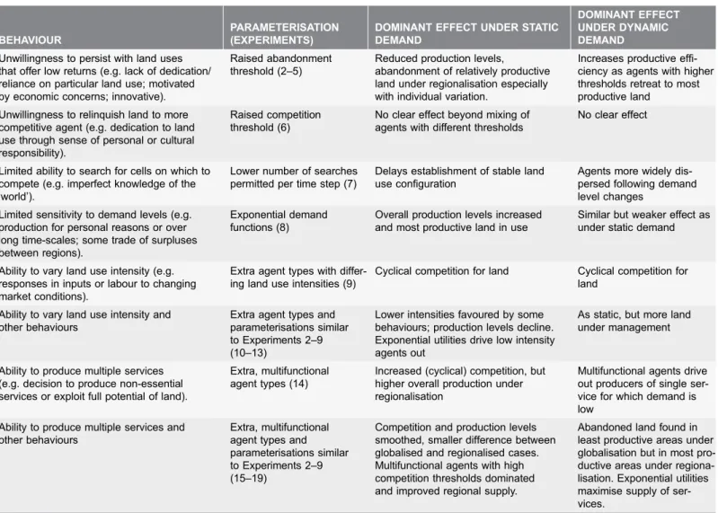
Table 5.Summary of the dominant effects of each form of behavioural variation investigated in the experiments (seeTable 2for further information on behavioural variations).
BEHAVIOUR
PARAMETERISATION (EXPERIMENTS)
DOMINANT EFFECT UNDER STATIC DEMAND
DOMINANT EFFECT UNDER DYNAMIC DEMAND Unwillingness to persist with land uses
that offer low returns (e.g. lack of dedication/ reliance on particular land use; motivated by economic concerns; innovative).
Raised abandonment threshold (2–5)
Reduced production levels,
abandonment of relatively productive land under regionalisation especially with individual variation.
Increases productive effi-ciency as agents with higher thresholds retreat to most productive land
Unwillingness to relinquish land to more competitive agent (e.g. dedication to land use through sense of personal or cultural responsibility).
Raised competition threshold (6)
No clear effect beyond mixing of agents with different thresholds
No clear effect
Limited ability to search for cells on which to compete (e.g. imperfect knowledge of the ‘world’).
Lower number of searches permitted per time step (7)
Delays establishment of stable land use configuration
Agents more widely dis-persed following demand level changes
Limited sensitivity to demand levels (e.g. production for personal reasons or over long time-scales; some trade of surpluses between regions).
Exponential demand functions (8)
Overall production levels increased and most productive land in use
Similar but weaker effect as under static demand
Ability to vary land use intensity (e.g. responses in inputs or labour to changing market conditions).
Extra agent types with differ-ing land use intensities (9)
Cyclical competition for land Cyclical competition for land
Ability to vary land use intensity and other behaviours
Extra agent types and parameterisations similar to Experiments 2–9 (10–13)
Lower intensities favoured by some behaviours; production levels decline. Exponential utilities drive low intensity agents out
As static, but more land under management
Ability to produce multiple services (e.g. decision to produce non-essential services or exploit full potential of land).
Extra, multifunctional agent types (14)
Increased (cyclical) competition, but higher overall production under regionalisation
Multifunctional agents drive out producers of single ser-vice for which demand is low
Ability to produce multiple services and other behaviours
Extra, multifunctional agent types and parameterisations similar to Experiments 2–9 (15–19)
Competition and production levels smoothed, smaller difference between globalised and regionalised cases. Multifunctional agents with high competition thresholds dominated and improved regional supply.
Abandoned land found in least productive areas under globalisation but in most pro-ductive areas under regiona-lisation. Exponential utilities maximise supply of ser-vices.
demands. Regionalisation of this system produced faster convergence but a less clear division between AFTs (Fig. 2b), as agents attempted to meet demands within each region and so utilised land that was less productive for their specific ES. In regions with low capital levels, areas occupied by each AFT remained distinct because supply could not match demand and, consequently, large differences in competitiveness occurred. In the most productive regions, however, demand could easily be satisfied and there was no inducement for agents to seek out the most productive cells. Some locations were abandoned as a result, and global supply (or production) was found to decline sharply (Fig. 2c).
When demand for recreation was suddenly reduced, both the globalised and regionalised systems adapted quickly (Table S1 in File S1). Conservationist agents abandoned a large number of cells (particularly in productive regions, under regionalisation, as only a few cells were needed to meet the reduced demand), and farmer agents took some of these cells over. Following this, as the supply of food approached demand levels and utility values for farmers declined, a smaller number of more productive cells, where farmers were still more likely to occur, were abandoned (increasing costs of land conversion would slow and, if large enough, prevent this by discouraging the adoption of more marginal cells) (Figs. 3a & b). Production of both services met or almost met demands in globalised and regionalised systems (Figs. 3c & d), though conservationists remained in areas of high natural amenity capital in the global case but only in areas of low natural amenity capital in the regional case (Figs. 3e & f). This was due to the differences in initial configurations and because individual agents had no reason to prefer production in a few productive cells over production in many marginal cells, as long as their thresholds for competition and abandonment were satisfied. Consequently land was predominantly abandoned in areas that were highly productive for both services in the regional case.
Figure 2. Baseline land use and supply levels results (Experiment 1) under constant levels of demand for services.Land use maps are shown for for Experiments 1a (a) and 1c (b) along with the corresponding supply of food produced in each (c).
Experiments 2–7 all showed a decline in total production levels and the establishment of sub-optimal land use configurations under different forms of modelled behaviour (some did, however, show faster convergence times following demand level changes). These experiments also revealed some specific and unexpected responses to regionalisation and dynamic demand levels (Table 5).
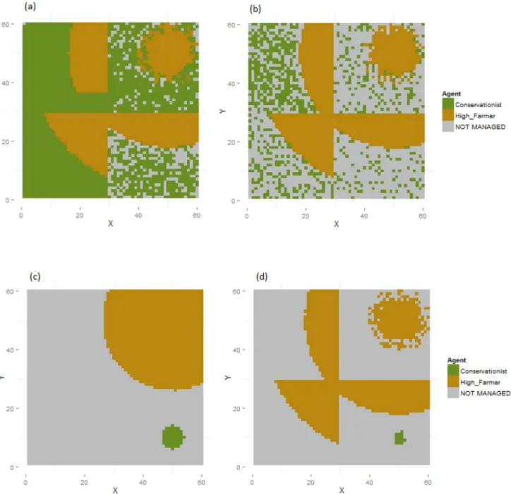
Increased typological abandonment thresholds (modelling an unwillingness to persist with low-utility land management; Experiments 2–5) restricted the land used by AFTs with higher thresholds, and consequently reduced total production levels (Figure 4). When demand levels for the AFT with the lowest threshold (in this case conservationists) dropped in a globalised world, that type abandoned land (in a single time-step) in an apparently random pattern. Under
regionalisation, the majority of abandoned land was highly productive (with high levels of natural amenity capital) (Fig. 4b). When demand levels for the AFT with the highest threshold (farmers) dropped, in contrast, agents of that type persisted primarily in the most productive cells (which they were already concentrated around), entirely abandoning every other region (Figs. 4c & 4d). This pattern of abandonment was reinforced by the tendency of high abandonment thresholds to discourage adoption of marginal cells, and did not occur under random
individual variation in abandonment or competition thresholds (Experiments 5 & 6; Fig. S1 in File S1).
The effect of limiting the search ability of agents (Experiment 7) was to delay the initial establishment of stable land use configurations (this is apparent visually, although our measure of convergence did not detect this due to large inter-simulation variability and the slow rate of change), and to produce less concentrated and distinct final agent distributions (Fig. S2 in File S1). When exponential utility functions were used to model the effects of agent insensitivity to demand levels or limited trade of regional surpluses (Experiment 8), the supply of ES was found to increase in all simulations, especially in the regional cases (Figs. 5a & 5b), where agent locations were influenced by productivity as well as regional demand. Productive regions therefore over-produced both ES (Figs. 5c & 5d), and no land was abandoned in any region.
The remaining simulations addressed the effects of variations in intensity and multi-functionality of land uses by adding additional AFTs to the simulated world. Experiment 9 established baseline results for the inclusion of mid- and low-intensity farmers (Table 4). In this experiment, both new AFTs were quickly eliminated from the global simulations following cyclical competition for marginal land, but mid-intensity farmers retained the least productive land in the regional simulations. Raising the abandonment thresholds of the original high-intensity AFTs (Experiment 10) and the competition thresholds of the new, lower
Figure 3. Baseline results (Experiment 1) following drop in demand for recreation.Final land use maps are shown for Experiments 1b (a) and 1d (b), following a drop in demand for recreation. The corresponding levels of demand and supply of food and recreation services are shown in (c) and (d) respectively. The distribution of conservationist agents in capital space is shown for Experiment 1b in (e) and for Experiment 1d in (f). Uniform grey areas of capital space in (e) and (f) do not occur in the modelled arena.
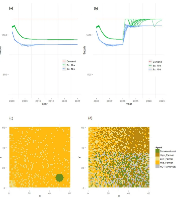
intensity AFTs (Experiment 11) allowed mid- and low-intensity farmers to manage a larger number of cells. This resulted in lower food production under static demand, but reduced abandonment of marginal land under dynamic demand because agents adapted land use intensity to local conditions (Fig. 6)
Figure 4. Effects of variation in abandonment thresholds (Experiments 2 & 3) on response to drop in demand for recreation.Final land use maps are shown for Experiments 2c (a), 2d (b), 3b (c) and 3d (d), showing the responses of conservationists to a drop in demand for recreation under different abandonment thresholds. Farmer agents have higher abandonment thresholds in Experiment 2 and conservationists in Experiment 3, respectively producing dispersed and concentrated patterns of conservationist land use.
Figure 5. Global and regional supply levels under decreased sensitivity to demand levels (Experiment 8).Global supply of food (a) and recreation (b) under dynamic recreation demand levels in Experiments 8b and 8d, and regional supply of food (c) and recreation (d) in Experiment 8d. Decreased sensitivity to demand levels is modelled through exponential utility functions, and resulted in overproduction in the most productive regions. Red lines are demand levels, which are shown following the drop in recreation demand in (c) and (d).
Figure 6. Supply levels and land use maps following the introduction of multifunctional agents.Supply of food in Experiment 10 under static demand (a) and dynamic demand for recreation (b), and final land use maps under global dynamic demand in Experiments 10b (c) and 11b (d), showing the difference in the response of conservationists to the drop in demand for recreation as their abandonment thresholds are varied.
(this effect was less marked under exponential utility functions, Experiments 12 and 13).
We next added multi-functionality to the simulations by allowing mid- and low-intensity farmers to supply recreation as well as food (but at lower total productivities than high-intensity agents; Table 4). In the baseline simulation (Experiment 14), this resulted in low intensity producers broadly specialising in areas of low productivity and, under dynamic demand, outcompeting conserva-tionists (Figs. S3a & S3b in File S1). Although agent locations and supply levels were not stable, the supply of both services under regionalisation was improved (Figs. S3c & S3d in File S1).
Raising the abandonment thresholds of high-intensity producers, without and with individual variation (Experiments 15 and 16 respectively), smoothed total productivities, reduced differences between global and regionalised productivities and slowed the pace of land use change (Fig. S4 in File S1; Table S1 in File S1). Regional production was maximised under uniform thresholds (and the
consequent absence of high intensity producers that could not satisfy their minimum utility values). Varying the thresholds of the lower intensity producers (Experiments 17 and 18) introduced greater variation within and between realisations, and led to domination by either high or medium and low-intensity producers. The difference between regionalised and globalised systems was minimised when competition thresholds were increased (Fig. S5 in File S1). The
Figure 7. Demand and supply levels with agent multifunctionality and reduced sensitivity to demand (Experiment 19).Food supply under static demand in Experiments 19a and 19c (a) and nature supply under dynamic demand in Experiments 19b and 19d (b). Supply of services exceeded demand throughout Experiment 19 except for regionalised supply of recreation under static demand.
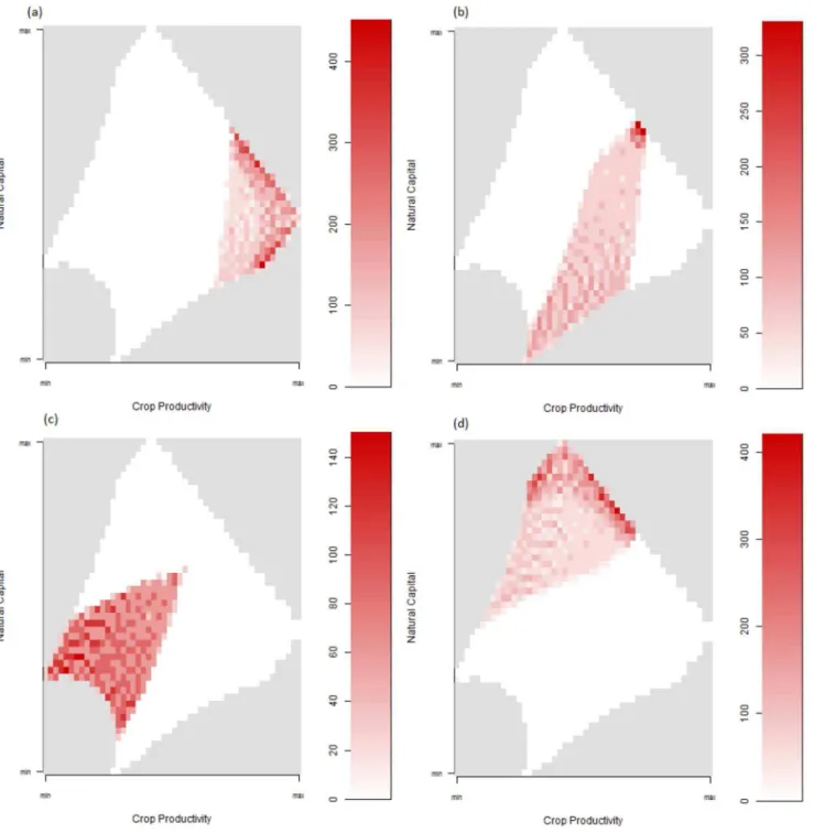
final experiment (19) combined multi-functional agents with exponential utility functions. This dramatically increased ES production in all systems, with supply far exceeding demand in almost all cases (Figs. 7a & 7b). AFTs were distributed according to capital levels and productive ability (Fig. 8), and these distributions
Figure 8. Agent locations in capital space in Experiment 19a.High-intensity farmers (a), mid-intensity farmers (b), low-intensity farmers (c) and conservationists (d), showing appropriate distributions relative to capital levels. Uniform grey areas do not occur in the modelled arena.
did not change substantially under dynamic demand. The configuration of land uses in the global case with static demands in this experiment represents a near-optimal outcome for the modelled system in terms of overall production levels.
Discussion
The level and security of food supplies at national, regional and global levels are crucial issues, not only in their own right, but also because of their implications for economies, livelihoods, land use patterns and the production of other essential ecosystem services [34,35]. In this study, we simulated contrasting production systems dedicated to maximising global food production or ensuring regional food security, and confronted these systems with sudden changes in demand levels and stylized models of human behaviour. These simulations allowed us to investigate some of the effects and trade-offs generated by each system in the presence of non-economically rational land manager behaviour and variations in land use intensity and multi-functionality, but in the absence of confounding effects that may occur in the real world.
The simulations presented here demonstrate that a completely globalised system of production can, in theory, supply more food from smaller areas of land than a system dedicated to ensuring regional food security. While regionalised systems did prevent the large-scale spatial separation of sites of supply and demand, they also generated overproduction in some regions and under-production in others, with the relatively productive locations at risk of
abandonment. Positive effects of global trade in food of the kind we find here are recognised [14], as are the negative effects of regionalisation or protectionism, which are known to include regional over-supply even under global shortages [11,17], the abandonment of productive land [9], and the maintenance of unproductive or inefficient land uses [36]. Nevertheless, the benefits of regionalisation that we find in terms of spatial provision of food and other ecosystem services are also recognised, and indeed underpin many policies that support regional or national production [8].
this was because managers could adapt their management to local conditions and potentially produce a wider range of services, as occurs in real land systems [39].
The strongest effect we found was that of raised abandonment thresholds (increased sensitivity to demand levels) under changing demand. Where we modelled a drop in demand affecting an AFT with a higher threshold, that type persisted only in the most productive areas, generating a highly concentrated pattern of land use and service provision. Where the demand drop affected an AFT with a lower threshold, however, agents became widely scattered, abandoning land in all areas and generating a fragmented pattern of land use with lower overall productive efficiency. Raised thresholds can describe any behaviour that makes land managers less willing or able to accept low returns on their activities (including the costs associated with the production of services or a change of land use). The dynamics we observed depend upon differences between types of land manager that are very likely to occur in reality; subsistence farmers, for example, have different priorities and costs, and so tolerate lower returns, than commercial farmers (e.g. [40]), while conservation is less sensitive to measurable returns than, say, forestry. We would therefore expect these groups to respond differently to changing demand levels, and this to result in different spatial configurations with strong implications for scale-dependent natural processes and service supply (e.g. [41,42]). This could potentially also apply to similar land uses located in regions which differ in social characteristics that affect support for land managers, suggesting that policies concerned with food security should take account of their economic, behavioural and cultural context.
We also find that the disadvantages of strict regionalisation are diminished or even reversed under modelled forms of behaviour. Variations in competition thresholds (making agents less likely to relinquish their land to another agent) describe behaviour that is frequently observed in real land managers, and make productivity differences between globalised and regionalised cases smaller. These differences are decreased further by the use of exponential utility functions. Such functions, in guaranteeing positive utility for the overproduction of a good or service, can represent a number of factors: insensitivity to demand on the part of land managers (because of differing motivations for production, personal capital levels, support networks or the temporal scale of production, amongst others) [16,43]; a failure of the trade system to transmit or express demand levels efficiently (e.g. [11]); or trade of surpluses beyond the boundaries of the modelled region or world (although there is an obvious limit to this ‘relaxed
regionalisation’, below which this finding simply restates the theoretical advantages of globalisation). The number of factors that can contribute to this effect, and the likelihood of their occurrence, suggest that regional food security may not cause drops in overall production levels of the size estimated when fully rational economic behaviour is assumed.
especially when ecosystem services are taken into account (e.g. [12,44,45]). Nevertheless, our findings suggest that its potential for increasing the supply and productivity of food and other ES may be large (beyond its obvious effects of increasing supply at local scales), and that it can represent a highly appropriate response to regionalisation in particular, allowing both production and security of supply to increase. It also appears to increase the sensitivity of the system to human behaviour and allow dramatic shifts in land use competitiveness, perhaps helping to explain the observed tendency of low-intensity producers to diversify when conditions are difficult [46,47].
Our findings, of course, are not directly transferable from our simple simulated setting to the real world, and inferences about real-world processes must take account of the identities and forms of the factors included and excluded from the model (for instance our exclusion of general political or economic barriers to land use change). Most fundamentally, true globalisation of demand and supply is impossible, physically and politically (and strict regionalisation highly improb-able), so that contrasting trade systems do not introduce or remove sensitivity of local land use to global factors, but instead vary the strength of this sensitivity [9]. Governments protect the interests of their own land managers and enact policies to preserve existing patterns of land use and ecosystem service supply, potentially constraining the ability of land managers to make ‘optimal’ decisions [7,48]. Global food markets are, as a result, highly complex and relatively inert,
comprising demands at many different spatial and temporal scales that produce ‘spaghetti bowls’ of (limited) free trade between specific partners (e.g. [49,50]). While some of our experiments might represent systems in which limited trade of surpluses occurs once regional supply levels are guaranteed, the complexities of more realistically structured systems could produce outcomes that differ
dramatically from those we find [51]. The study of idealised theoretical systems at the extremes of the globalisation-regionalisation continuum allows us to
understand basic characteristics of these systems that can inform interpretation of real-world phenomena, but such interpretation must be done with care.
In any case, globalisation is a rapid and continuing process, and globally-traded agricultural products increased in value from $32 billion in 1961 to $442 billion in 2002 [58]. Equally, human behaviour is known to be capable of confounding drivers of land use change and, more broadly, generating counter-intuitive systemic effects across apparently predictable systems [10,19,60,61]. Our findings that various forms of land manager behaviour can dramatically alter the basic effects of complete globalisation and regionalisation of demand in a simulated setting are therefore highly relevant to current processes of land use change, particularly where the rate of change and implications for food supply, landscape heterogeneity, spatial provision of ecosystem services and the resilience of existing land uses are of concern.
Conclusions
We find a number of strong effects of modelled land manager behaviour on stylised land use systems in globalised and regionalised settings. The most important of these include:
N
Reductions in overall productivity, but increases in production per unit area, under globalisation, and increases in overall productivity under regionalisation, reducing the productivity gap between globalised and regionalised systems.N
Stabilisation of the land use system, with responses to changes in demand levels for ecosystem goods or services being reduced and/or slowed.N
A clear divergence in system-wide responses when sensitivity to demand levels varies between types of land managers, resulting either in concentration or fragmentation of similar land uses as demand levels change.N
The adaptation of land use intensity and multi-functionality to match local conditions, improving the spatial delivery of ecosystem services and overall productive efficiencies and totals.The consequences of these effects for the production of food and other ecosystem goods and services are significant and, while our findings are only directly applicable to isolated behaviours in a simulated setting, clearly suggest that studies of land use change should take careful account of individual behaviour within the wider context.
Supporting Information
Author Contributions
Conceived and designed the experiments: CB DMR JV SA PV MR. Performed the experiments: CB. Analyzed the data: CB. Wrote the paper: CB DMR JV SA PV MR.
References
1. McKenzie LW (1953) Specialisation and efficiency in world production. Review Econ Studies 21(3): 165–180.
2. Hertel TW(2011) The Global Supply and Demand for Agricultural Land in 2050: A Perfect Storm in the Making? Am J Agr Econ 93(2): 259–275.
3. Anderson K (2010). Globalization’s effects on world agricultural trade, 1960–2050. Philosophical Transactions of the Royal Society of London. Series B, Biological Sciences, 365(1554), 3007–21.
4. Hay DA (2001) The Post-1990 Brazilian Trade Liberalisation and the Performance of Large Manufacturing Firms: Productivity, Market Share and Profits. The Economic Journal 111(473): 620–641.
5. Thangavelu SM, Toh M-H(2005) Bilateral ‘‘WTO-Plus’’ Free Trade Agreements: The WTO Trade Policy Review of Singapore 2004. The World Economy 28(9): 1211–1228.
6. Subramanian A, Wei S-J(2007) The WTO promotes trade, strongly but unevenly. J Int Econ 72(1): 151–175.
7. Potter C, Burney J(2002) Agricultural multifunctionality in the WTO—legitimate non-trade concern or disguised protectionism? J Rural Stud 18(1): 35–47.
8. Dibden J, Cocklin C (2009) ‘‘Multifunctionality’’: trade protectionism or a new way forward? Environ Plann A 41(1): 163–182.
9. Lambin EF, Meyfroidt P(2011) Global land use change, economic globalization, and the looming land scarcity. P Natl Acad Sci USA 108(9): 3465–72.
10. Potter C, Tilzey M (2005) Agricultural policy discourses in the European post-Fordist transition: neoliberalism, neomercantilism and multifunctionality. Prog Hum Geog 29(5): 581–600.
11. Stoate C, Boatman ND, Borralho RJ, Carvalho CR, de Snoo GR, et al.(2001). Ecological impacts of arable intensification in Europe. J Env Manag 63(4): 337–365.
12. Otte A, Simmering D, Wolters V (2007) Biodiversity at the landscape level: recent concepts and perspectives for multifunctional land use. Landscape Ecology 22: 639–642.
13. Robertson GP, Swinton SM(2005) Reconciling agricultural productivity and environmental integrity: a grand challenge for agriculture. Front Ecol Environ 3(1): 38–46.
14. Godfray HCJ, Beddington, JR, Crute, IRHaddad L, Lawrence D, et al. (2010) Food security: the challenge of feeding 9 billion people. Science 327(5967): 812–8.
15. van Vliet J, de Groot HLF, Rietveld P, Verburg PH(2014). Manifestations and underlying drivers of agricultural land use change in Europe. Landscape and Urban Planning 133, 24–36.
16. Siebert R, Toogood M, Knierim A (2006) Factors Affecting European Farmers’ Participation in Biodiversity Policies. Sociologia Ruralis 46(4): 318–340.
17. Walford N (2003) Productivism is allegedly dead, long live productivism. Evidence of continued productivist attitudes and decision-making in South-East England. J Rural Stud 19(4): 491–502.
18. Alexander P, Moran D, Rounsevell MDA, Smith P(2013) Modelling the perennial energy crop market: the role of spatial diffusion. J R Soc Interface 10(88): 20130656.
19. Weisbuch G, Boudjema G(1999) Dynamical Aspects in the Adoption of Agri-Environmental Measures. Advances in Complex Systems 02(01): 11–36.
21. Mughan A, Bean C, McAllister I(2003) Economic globalization, job insecurity and the populist reaction. Electoral Studies 22(4): 617–633.
22. Parker DC, Hessl A, Davis SC (2008) Complexity, land-use modeling, and the human dimension: Fundamental challenges for mapping unknown outcome spaces. Geoforum 39(2): 789–804.
23. Olesen JE, Bindi M(2002) Consequences of climate change for European agricultural productivity, land use and policy. Eur J Agron 16(4): 239–262.
24. Goklany IM(1995) Strategies to enhance adaptability: Technological change, sustainable growth and free trade. Climatic Change 30(4): 427–449.
25. Matthews RB, Gilbert NG, Roach A, Polhill JG, Gotts NM(2007). Agent-based land-use models: a review of applications. Landscape Ecology 22(10): 1447–1459.
26. Rounsevell MDA, Pedroli B, Erb KH, Gramberger M, Busck AG, et al.(2012) Challenges for land system science. Land Use Policy 29(4): 899–910.
27. Magliocca NR, Brown DG, Ellis EC(2013) Exploring Agricultural Livelihood Transitions with an Agent-Based Virtual Laboratory: Global Forces to Local Decision-Making. PLoS ONE 8(9): e73241.
28. Feng L, Li B, Podobnik B, Preis T, Stanley HE(2012) Linking agent-based models and stochastic models of financial markets. PNAS 109(22): 8388–8393.
29. Murray-Rust D, Brown C, van Vliet J, Alam SJ, Robinson DT, et al. (2014). Combining Agent Functional Types, capitals and services to model land use dynamics. Environmental Modelling and Software 59: 187–201.
30. Arneth A, Brown C, Rounsevell M(2014) Global models of human decision-making for land-based mitigation and adaptation assessment. Nature Climate Change 4: 550–557.
31. Murray-Rust D, Dendoncker N, Dawson TP, Acosta-Michlik L, Karali E, et al.(2011) Conceptualising the analysis of socio-ecological systems through ecosystem services and agent-based modelling. J Land Use Science 6(2–3): 83–99.
32. Winch P(1958) The idea of a social science and its relation to philosophy, London: Routledge.
33. Helbing D(2010) Quantitative Sociodynamics: Stochastic Methods and Models of Social Interaction Processes. Berlin: Springer-Verlag.
34. Swaffield S, Primdahl J(2006) Spatial concepts in landscape analysis and policy: some implications of globalisation. Landscape Ecology 21: 315–331.
35. Concepcin ED, Dı´az M, Baquero RA (2008) Effects of landscape complexity on the ecological effectiveness of agri-environment schemes. Landscape Ecology 23: 135–148.
36. Bulte EH, Damania R, Lo´pez R (2007). On the gains of committing to inefficiency: Corruption, deforestation and low land productivity in Latin America. J Environ Econ Manag 54(3): 277–295.
37. Jager W, Janssen MA, De Vries HJM, De Greef J, Vlek CAJ(2000). Behaviour in commons dilemmas: Homo economicus and Homo psychologicus in an ecological-economic model. Ecological Economics 35(3): 357–379.
38. Schreinemachers P, Berger T (2006) Land use decisions in developing countries and their representation in multi-agent systems. J Land Use Sci 1(1): 29–44.
39. Lambin EF, Rounsevell MD, Geist HJ(2000) Are agricultural land-use models able to predict changes in land-use intensity? Agric Ecosys Environ 82(1–3): 321–331.
40. Shackleton CM, Shackleton SE, Cousins B (2001) The role of land-based strategies in rural livelihoods: The contribution of arable production, animal husbandry and natural resource harvesting in communal areas in South Africa. Dev Southern Africa 18(5): 581–604.
41. Plieninger T (2006) Habitat loss, fragmentation, and alteration – quantifying the impact of land use changes on a Spanish dehesa landscape by use of aerial photography and GIS. Landscape Ecology 21: 91–105.
42. Bolliger J, Kiensat F, Soliva R, Rutherford G(2007) Spatial sensitivity of species habitat patterns to scenarios of land use change (Switzerland). Landscape Ecology 22: 773–789.
44. Pretty J (2008) Agricultural sustainability: concepts, principles and evidence. Philos T Roy Soc B, Biological sciences 363(1491): 447–65.
45. Zasada I(2011). Multifunctional peri-urban agriculture—A review of societal demands and the provision of goods and services by farming. Land Use Policy 28(4): 639–648. doi:10.1016/
j.landusepol.2011.01.008
46. De Janvry A, Sadoulet E, De Anda GG (1995) NAFTA and Mexico’s maize producers. World Development 23(8): 1349–1362.
47. Batterbury S(2001) Landscapes of Diversity: A Local Political Ecology of Livelihood Diversification in South-Western Niger. Cultural Geographies 8(4): 437–464.
48. Yeates N (2002) Globalization and social policy: from global neoliberal hegemony to global political pluralism. Global Social Policy 2(1): 69–91.
49. Baldwin RE(2006) Multilateralising Regionalism: Spaghetti Bowls as Building Blocs on the Path to Global Free Trade. The World Economy 29(11): 1451–1518.
50. Anderson K(2009) Distortions to agricultural incentives: A global perspective, 1955–2007. London: Palgrave Macmillan and Washington DC: World Bank.
51. Sheppard E(2011) Geographical political economy. J Econ Geog 11(2): 319–331.
52. Van Meijl H, van Rheenen T, Tabeau A, Eickhout B(2006). The impact of different policy environments on agricultural land use in Europe. Ag Ecosys Environ 114(1): 21–38.
53. Verburg PH, Mertz O, Erb K-H, Haberl H, Wu W (2013). Land system change and food security: towards multi-scale land system solutions. Current Opinion in Environmental Sustainability 5: 494–502.
54. Tilman D, Cassman KG, Matson PA, Naylor R, Polasky S (2002) Agricultural sustainability and intensive production practices. Nature 418(6898): 671–7.
55. Burfisher ME, Robinson S, Thierfelder K(2001) The Impact of NAFTA on the United States. J Econ Perspect 15(1): 125–144.
56. Fortin E(2005) Reforming Land Rights: The World Bank and the Globalization of Agriculture. Social & Legal Studies 14(2): 147–177.
57. Semwal RL, Nautiyal S, Sen KK, Rana U, Maikhuri RK, et al. (2004) Patterns and ecological implications of agricultural land-use changes: a case study from central Himalaya, India. Agric Ecosys Environ 102(1): 81–92.
58. Wu¨ rtenberger L, Koellner T, Binder CR (2006) Virtual land use and agricultural trade: Estimating environmental and socio-economic impacts. Ecological Economics 57(4): 679–697.
59. Menezes F(2001). Food Sovereignty: A vital requirement for food security in the context of globalization. Development 44(4), 29–33.
60. Helbing D, Brockman D, Chadefaux T, Donnay K, Blanke U, et al.(2014) Saving Human Lives: What Complexity Science and Information Systems can Contribute. Journal of Statistical Physics DOI 10.1007/s10955-014-1024-9