Article
Commonality in structure among food web networks
Carrie J. Byron1, Craig Tennenhouse2 1
Department of Marine Sciences, University of New England, 11 Hills Beach Road, Biddeford, ME 04005, USA 2
Department of Mathematical Sciences, University of New England, 11 Hills Beach Road, Biddeford, ME 04005, USA E-mail: [email protected], [email protected]
Received 15 July 2015; Accepted 15 August 2015; Published online 1 December 2015
Abstract
A goal of this study was to determine similarities in structure among food webs that are otherwise disparate with regard to species, population, and size. Food webs were examined as directed, unweighted graphs in order to normalize food webs with regard to biomass and population/species distinctions. The graphs were further normalized with regard to topological size and existence of circuits through the reduction of each strongly connected component to a single node. This had the added benefit of resulting in networks with more clear delineation between trophic levels. Finally, common induced subgraphs were considered for their obvious value in characterizing network structure. Through this study we determined not only that there are pairs of systems that are highly similar in structure once appropriately normalized for size, makeup, and geographical location, but also that a majority of food webs have similar structural components when compared with random food webs.
Keywords network ecology; graph theory; food webs; directed graphs.
1 Introduction
Ecosystems are complex. Management of ecosystems for environmental and societal goods and services can be even more complex. Finding commonalities and patterns in this complexity will help streamline management efforts. The complexity in ecosystems can be captured in its food web which describes predator prey relationships and flow of energy between species.
Food webs are one type of network that has been subject to examination through the founding disciplines of network ecology and graph theory. Dunne (2002, 2004, 2009) has done much work characterizing network structure of food webs demonstrating the role of connectedness, size, and robustness. Food webs, like most real world networks, are not random (Williams and Martinez, 2000). Food webs from different types of ecosystems share fundamental structural and ordering characteristics (Dunne et al., 2004).
Network Biology ISSN 22208879
URL: http://www.iaees.org/publications/journals/nb/onlineversion.asp RSS: http://www.iaees.org/publications/journals/nb/rss.xml
Email: [email protected] EditorinChief: WenJun Zhang
IAEES www.iaees.org Finding ways to describe and quantify these fundamental structural and ordering characteristics can be challenging due to the complexity of the food webs. Several metrics and techniques have already been developed in the field of network ecology. Here we attempt to advance this field by proposing a methodology for examining commonality among food web models that is strongly rooted in graph theory and builds from prior work of Allesina et al. (2005).
We focus on “wet” food webs, including marine, brackish, and freshwater systems from around the world and propose a set of metrics derived from graph theory that can be used to evaluate similarities and differences across these complex systems. Using a combined graph theory and network ecology approach, we first establish that, like other real-world networks, food webs have more organization than randomly generated webs (Watts and Strogatz, 1998; Williams and Martinez, 2000). We then test for similarities and differences across all food web types to examine whether there are mathematical properties of food webs that are ubiquitous around the world.
Our approach is advancement over other studies because of our large sample size (21) and ecosystem diversity (i.e. fresh-water, estuarine, marine). Many other comparative studies of food webs only look at 3-5 networks and are typically all a similar type of ecosystem (Allesina et al., 2005; Bascompte and Melián, 2005; Dunne et al., 2004). We also examined larger subgraph structures (up to 7 nodes) compared to other studies (3 nodes) (Borrelli, 2015).
2 Method
We will use the following terminology throughout this manuscript.
Definition: A directed graph (henceforth referred to as a graph) is an ordered pair of sets (V, E) of vertices (or
nodes) V and edges E. Each edge e in E is itself an ordered pair (u, v) of distinct elements from V, (i.e. we do not allow loops or multiple edges, but circuits of length 2 are permitted). The in-degree (alternatively out-degree) of a node v in a graph G is the number of edges in G of the form (x, v) (alternatively (v, x)) for any vertex x in G.
Definition: A graph G is connected if, for every pair u,v of vertices in G, there is a set of edges in G (e1, e2,…,en) such that u is in e1, v is in en, and for each i the edges ei and ei+1 have a non-empty intersection. Definition: An n-path is a connected graph on n vertices in which one vertex has out-degree 1 and in-degree 0 (the source), one vertex has out-degree 0 and in-degree 1 (the sink), and the remaining vertices each have in-degree and out-in-degree 1. An n-circuit is a connected graph on n vertices in which each vertex has both in-degree and out-in-degree 1. A graph that contains no circuit is acyclic.
Definition: A graph G = (VG, EG) is an induced subgraph of a graph H = (VH, EH) if there is an injective
function f from VG to VH such that for any edge (u, v) in EG the corresponding edge (f(u), f(v)) is in EH, and if (u, v) is not an edge in EG then (f(u), f(v)) is not an edge in EH.
As an example, the 4-path is not an induced subgraph of the 4-circuit, but it is an induced subgraph of the n -circuit for all n> 4.
Definition: The order of a graph G is the number of vertices in G, denoted n(G). Its size e(G) is the number of edges in G.
2.1 Food web networks
predator in the food web. Each Ecopath food web was created by different researchers for different purposes and therefore has unique classifications and groupings of species (Table 2). To standardize these diverse models, each food web was given two treatments prior to any analysis: (1) removal of detritus and (2) removal of circuits.
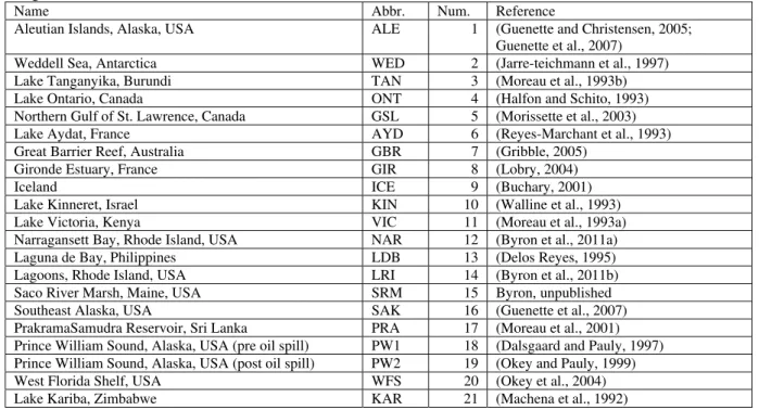
Table 1 Networks used in analysis. Networks published prior to 2010 were downloaded from the Ecopath website (www.ecopath. org). All networks were assigned both a three letter abbreviation (Abbr.) and a number (Num.) that is used in subsequent tables and figures.
Name Abbr. Num. Reference
Aleutian Islands, Alaska, USA ALE 1 (Guenette and Christensen, 2005; Guenette et al., 2007)
Weddell Sea, Antarctica WED 2 (Jarre-teichmann et al., 1997) Lake Tanganyika, Burundi TAN 3 (Moreau et al., 1993b) Lake Ontario, Canada ONT 4 (Halfon and Schito, 1993) Northern Gulf of St. Lawrence, Canada GSL 5 (Morissette et al., 2003) Lake Aydat, France AYD 6 (Reyes-Marchant et al., 1993) Great Barrier Reef, Australia GBR 7 (Gribble, 2005)
Gironde Estuary, France GIR 8 (Lobry, 2004)
Iceland ICE 9 (Buchary, 2001)
Lake Kinneret, Israel KIN 10 (Walline et al., 1993) Lake Victoria, Kenya VIC 11 (Moreau et al., 1993a) Narragansett Bay, Rhode Island, USA NAR 12 (Byron et al., 2011a) Laguna de Bay, Philippines LDB 13 (Delos Reyes, 1995) Lagoons, Rhode Island, USA LRI 14 (Byron et al., 2011b) Saco River Marsh, Maine, USA SRM 15 Byron, unpublished Southeast Alaska, USA SAK 16 (Guenette et al., 2007) PrakramaSamudra Reservoir, Sri Lanka PRA 17 (Moreau et al., 2001) Prince William Sound, Alaska, USA (pre oil spill) PW1 18 (Dalsgaard and Pauly, 1997) Prince William Sound, Alaska, USA (post oil spill) PW2 19 (Okey and Pauly, 1999) West Florida Shelf, USA WFS 20 (Okey et al., 2004) Lake Kariba, Zimbabwe KAR 21 (Machena et al., 1992)
Table 2 Metadata describing the motivation for creating the food web model and the different emphasis on species groupings in each study system. See Table 1 for full ecosystem names associated with the first column, ‘ Abbr.’. ‘Percent of FW nodes aggregated’ is the number of species groups that contain multiple species divided by the total number of species groups in the original food web model, as defined by the author, ‘FW nodes’. ‘RAM nodes’ is the number of nodes in the RAM after removing cyclicity and detritus.
Abbr. Study Goal Species Focus FW
nodes
Percent of FW nodes aggregated
RAM nodes
ALE Evaluate whether predation by killer whales might explain the decline of Steller sea lions in the central and western Aleutian Islands.
Steller sea lion and their principal prey species
40 60% 34
WED Integrate the results of the various research efforts directed towards the shelf communities into a coherent whole.
dominant groups of benthic shelf
community 20 100% 15
TAN Quantify the food web and the production of pelagic fish and invertebrates.
pelagic fish and invertebrates 7 100% 4
ONT Characterize the food web. Phytoplankton, zooplankton, benthos were aggregated. Fish, mysid, amphipod species were left independent.
14 29% 13
GSL Impact of groundfish collapse. phytoplankton and detritus to marine mammals and seabirds, including harvested species of pelagic, demersal,
IAEES www.iaees.org and benthic domains
AYD Understand functioning of eutorophic
ecosystem. emphasis on two dominat fish species, perch (Percafluviatilis) and roach
(Rutilusrutilus)
11 82% 10
GBR Identify the effects of the major fisheries in (1) mangrove, (2) lagoon-seagrass, and (3) coral reef systems, and the possible confounding effects of independently developed fisheries management plans.
fish and prawn 32 75% 8
GIR Improve understanding of the
complexity of estuarine ecosystems and response to various pressures.
estuarine fish 18 89% 17
ICE Describe North Atlantic marine ecosystem with fisheries prior to expansion of large-scale commercial fisheries.
two primary producer groups, five invertebrate groups, twelve fish groups (including one juvenile group for cod), one seabirds group, three marine mammals groups and one detritus group
24 63% 20
KIN Characterize the food web. Good data for biomass and production of phytoplankton and zooplankton and diet and catches of main fish species.
14 71% 13
VIC Evaluate change in dynamics of fish community after introduction of Nile perch.
fish-centric model 16 75% 12
NAR Calculate carrying capacity for shellfish aquaculture.
Includes all trophic levels with emphasis on filter feeders.
15 93% 14
LDB Text not available, only data tables Text not available, only data tables 17 71% 15
LRI Calculate carrying capacity for shellfish aquaculture.
Includes all trophic levels with emphasis on filter feeders.
16 88% 15
SRM Characterize the food web. fish and birds 29 62% 27 SAK Understand why sea lions increased in
the presence of killer whales in Southeast Alaska.
Steller sea lion and their principal prey species
40 68% 19
PRA Describe trophic relationships and
importance of unexploited fish stocks. commercial fisheries and introduced tilapiine fish 17 71% 16 PW1 Characterize trophic interactions prior to
oil spill.
not fish-centric, plankton to mammals 19 95% 18
PW2 Understand structure and functional characteristics of food web after oil spill.
primary producers, zooplankton, benthic invertebrates, planktivorous 'forage fishes', larger fishes, birds, mammals, and detritus
48 73% 13
WFS Community effects of seafloor shading by plankton blooms.
primary producers 59 92% 6
KAR Assess trophic interrelationships and
community structure. Trophic groups selected based on known importance and availability of data from the literature. Some groups were left out because of perceived minor importance for overall trophic flows. Some fish species were grouped both because commercial landing statistics do not separate individuals species and also because their biology is similar.
10 70% 9
2.2 RAM generation process
Despite the unique species groupings in each web, there is one exception - detritus. Every Ecopath model must include a detritus (decaying organic matter) component. Detritus is used to capture any unused energy in the ecosystem and in that way is common across all webs. The vertex with this detritus label shares at least one edge with every other vertex in each food web. Because we are interested in examining similarities and differences across food webs, the detritus vertex was removed from every food web. What remains from FW is
It is common that food webs contain circuits whereby energy flows cyclically between specific predator and prey groups, typically across 2 adjacent trophic levels. Because we are interested in how energy moves across multiple trophic levels, smaller circuits such as these become less consequential. Cycles or hereafter, circuits, in F are located and reduced to a single vertex, resulting in a reduced acyclic model (RAM) of the food
web (see Allesina et al. 2005 for another treatment of reduced acyclic graphs). The resulting 21 RAMS are
more uniform in size than the graphs in FW and contain fewer vertices, leading to simpler computational
analysis.
2.3 Random RAM generation process
Because one of our goals is to find properties of networks that are unique to food webs, random graphs were created for comparison. Each graph F in FW has a density d(F), the ratio of the number of edges to n(F)(n(F)+1). Note that n(F)(n(F)+1) is the maximum number of edges in a graph on n(F)+1 vertices. A
random graph on n(F)+1 vertices was generated through inclusion of each potential edge among each pair of
vertices with probability equal to d(F). The resulting graph is then stripped of a vertex of highest total degree
(i.e. the sum of in-degree and out-degree). What results is a graph RF with the same order as and similar
density to F. The set of all graphs of the form RF is denoted RFW. Each graph in RFW undergoes the RAM
generation process, described above, to result in a random equivalent of each RAM, or an RRAM.
2.4 Induced subgraphs
There exist 243,262 graphs on up to 7 nodes that are acyclic and connected, which were placed into array A.
Each graph in A was examined for inclusion in each RAMR as an induced subgraph, resulting in a binary array AR. These binary arrays were subsequently added component-wise and the resulting array At, with integer
components between zero and 21 inclusive, was generated. The array At is an indicator of occurrence for each
graph in A among the RAMS. Graphs from A with at least five vertices were examined for high occurrence.
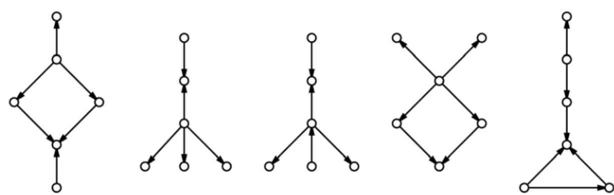
Those that appeared often were included in a set which we will refer to as S, consisting of induced subgraphs
of approximately two-thirds of the RAMS examined (Fig. 1). It was discovered that no graph in A with greater
than 6 nodes is an induced subgraph of a significant number of RAMS. Connected, acyclic graphs with more
than 6 nodes did not appear as induced subgraphs with high enough frequency to be studied. Next, each graph in S was examined for its inclusion in each RRAM.
2.5 Network metrics
To examine similarities and differences across food webs, individual metrics of each FW and RAM were
calculated and standardized against the metrics of order or size. The eight metrics listed in Table 3 were used for cluster and principle component analyses. Each metric captures a unique quality of the networks useful for examining similarities and differences across ecosystems.
We define some relevant graph theoretic terms below
Definition: The clique number of a graph is the order of the largest complete subgraph. An undirected graph is complete if each vertex is adjacent to every other vertex.
Definition: The connectivity (alternatively edge-connectivity) of a graph is the fewest number of vertices (edges) the removal of which results in a disconnected graph.
Definition: A graph’s density is the ratio of its size to the maximum possible number of edges among its vertices.
Definition: The distance between vertices u,v in a graph G is the length of the shortest path from u to v. The
diameter of G is the length of the greatest distance. If there are vertices with no path between them then the
IAEES www.iaees.org Definition: An independent set is a collection of vertices with no adjacencies among one other.
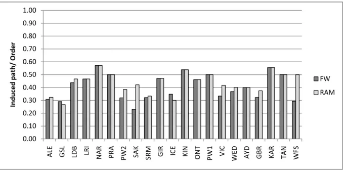
Definition: An induced path is simply an induced graph in the form of a path. That is, no vertex along the path is adjacent to any other besides its neighbors along the path.
Definition: The eccentricity of a vertex v is the greatest distance from v to any other vertex in a graph. The
radius of a graph is the lowest eccentricity.
Fig. 1 The five six-node graphs below are those that appear in 14 RAMS (Fig. 1a) and 13 RAMS (Figs. 1b-1e). None of the graphs
in Fig. 1 appear as induced subgraphs in any of the RRAMS.
2.6 Cluster analysis
A cluster analysis was performed to examine relatedness among food webs. Clusters are based on the shortest Euclidean distances between computed metrics. The resulting dendrogram plot is of the hierarchical binary cluster tree where the height of the U-shaped bars are the distances (y-axis) between networks (x-axis) being connected.
2.7 PCA
A Principle Component Analysis (PCA) was performed to examine relationship between metrics. Since variances among metrics were similar due to standardizing against order or size, raw data was used to perform the PCA. The first principal component and second principal component were plotted for each network for both food webs and RAMS. A biplot of the principal component coefficients showing variables represented as
vectors. This biplot allows visualization of the magnitude and sign of each variable’s contribution to the first two principal components, and how each observation is represented in terms of those components.
3 Results
3.1 Induced subgraphs
No graph in S was found as an induced subgraph in any RRAM. It was determined that each RRAM is much
smaller than the RAMS. Ecologically, the naturally-occurring RAMS have a more complex structure than
randomized ones, and naturally-occurring food webs appear to have much lower cyclicity than randomized food webs.
Large graphs that were found to be induced subgraphs of a majority of RAMS, i.e. the graphs in S, were
not represented in all RAMS. There are five systems in which no graph from S appeared as an induced
subgraph (Lake Tanganyika in Burunidi, Lake Aydat in France, the Great Barrier Reef in Australia, West Florida Shelf in USA, Lake Kariba in Zimbabwe) (Table 3). The remaining 16 RAMS did contain at least one
induced subgraph from the set S, and 9 of those RAMS contained all 5 common induced subgraphs (Aleutians
Rhode Island coastal lagoons in USA, Saco River estuary marsh in USA, Southeast Alaska, Lake Prakrama Samudra in Sri Lanka, and Prince William Sound Alaska prior to the oil spill) (Table 3). There appears to be no geographic or environmental pattern to the number of these common induced subgraphs a network contains (Fig. 2).
Table 3 Metrics computed for each Food Web (FW) and RAM. Metrics were standardized by order or edges making all values a relative proportion. The number of induced subgraphs for each network is specified in the first column, Ind. Sub. Networks either contained all 5 of the listed induced subgraphs (5), at least one induced subgraph (1+), or no induced subgraphs. Network names are listed in Table 1.
Ind. Sub.
Network Abbr. Num.
clique number/
order (undirected)
connectivity/
order (undirected)
density (edges/ max
possible edges)
edge
connectivity/ edges (undirected)
finite diameter/
order
independent
set/ order (undirected)
induced path/
order (undirected)
radius/ order
(undirected)
FW RAM FW RAM FW RAM FW RAM FW RAM FW RAM FW RAM FW RAM 5
ALE 1 0.28 0.29 0.00 0.06 0.44 0.44 0.00 0.01 0.10 0.09 0.33 0.35 0.31 0.32 0.00 0.06
5
GSL 5 0.29 0.30 0.16 0.17 0.60 0.60 0.02 0.02 0.10 0.10 0.29 0.30 0.29 0.27 0.06 0.07
5
LDB 13 0.25 0.27 0.00 0.07 0.35 0.40 0.00 0.02 0.19 0.20 0.50 0.47 0.44 0.47 0.00 0.13
5
LRI 14 0.27 0.27 0.13 0.13 0.37 0.37 0.05 0.05 0.13 0.13 0.40 0.40 0.47 0.47 0.13 0.13
5
NAR 12 0.36 0.36 0.21 0.21 0.46 0.46 0.07 0.07 0.14 0.14 0.36 0.36 0.57 0.57 0.14 0.14
5
PRA 17 0.19 0.19 0.13 0.13 0.40 0.40 0.04 0.04 0.13 0.13 0.44 0.44 0.50 0.50 0.13 0.13
5
PW2 19 0.15 0.38 0.06 0.08 0.32 0.47 0.01 0.03 0.11 0.23 0.32 0.54 0.32 0.38 0.04 0.08
5
SAK 16 0.33 0.32 0.00 0.11 0.60 0.47 0.00 0.02 0.10 0.16 0.26 0.37 0.23 0.42 0.00 0.11
5
SRM 15 0.18 0.19 0.04 0.04 0.24 0.24 0.01 0.01 0.11 0.11 0.50 0.48 0.32 0.33 0.07 0.07
1+
GIR 8 0.29 0.29 0.06 0.06 0.38 0.38 0.02 0.02 0.18 0.18 0.41 0.41 0.47 0.47 0.12 0.12
1+
ICE 9 0.48 0.55 0.04 0.05 0.62 0.63 0.01 0.01 0.09 0.10 0.22 0.25 0.35 0.30 0.09 0.10
1+
KIN 10 0.31 0.31 0.08 0.08 0.42 0.42 0.03 0.03 0.23 0.23 0.46 0.46 0.54 0.54 0.15 0.15
1+
ONT 4 0.23 0.23 0.23 0.23 0.38 0.38 0.10 0.10 0.15 0.15 0.54 0.54 0.46 0.46 0.15 0.15
1+
PW1 18 0.28 0.28 0.11 0.11 0.35 0.35 0.04 0.04 0.17 0.17 0.44 0.44 0.50 0.50 0.11 0.11
1+
VIC 11 0.60 0.50 0.33 0.42 0.75 0.68 0.06 0.11 0.13 0.17 0.33 0.42 0.33 0.42 0.07 0.08
1+
WED 2 0.26 0.27 0.05 0.07 0.29 0.28 0.02 0.03 0.21 0.20 0.47 0.53 0.37 0.40 0.11 0.13
0
AYD 6 0.60 0.60 0.40 0.40 0.71 0.71 0.13 0.13 0.20 0.20 0.40 0.40 0.40 0.40 0.10 0.10
0
GBR 7 0.29 0.50 0.13 0.25 0.49 0.61 0.02 0.18 0.26 0.25 0.29 0.50 0.32 0.38 0.06 0.13
0
KAR 21 0.33 0.33 0.11 0.11 0.39 0.39 0.07 0.07 0.22 0.22 0.44 0.44 0.56 0.56 0.22 0.22
0
TAN 3 0.83 1.00 0.67 0.75 1.07 1.00 0.25 0.50 0.33 0.25 0.33 0.25 0.50 0.50 0.17 0.25
0
IAEES
Fig. 2 Map the numbe
3.2 Netw Metric va standardi
Fig. 3 a
0 0 0 0 0 0 0 0 0 0 1
Clique
number
Order
p of the world s er of the five co
work metrics alues were si ized against o
0.00 0.10 0.20 0.30 0.40 0.50 0.60 0.70 0.80 0.90 1.00
ALE GSL
showing geogra ommon induced
s
milar for both order or size,
LDB LRI NAR
aphic locations d subgraphs in e
h food webs there was low
PRA PW2 SAK
of all the netwo each network.
and RAMS ac
w variance ac
SRM GIR ICE KIN
orks used in the
cross most ne cross the metr
KIN
ONT PW1 VIC
e study. Colored
etworks (Fig. rics.
VIC
WED AYD GBR
w
d dots are shade
3). Because
KAR TAN WFS
www.iaees.org
ed according to
metrics were
FW
RAM
o
Fig. 3 b
Fig. 3 c
Fig. 3 d
0.00 0.10 0.20 0.30 0.40 0.50 0.60 0.70 0.80 0.90 1.00
ALE GSL LDB LRI NAR PRA PW2 SAK SRM GIR ICE KIN
ONT PW1 VIC WED AYD GBR KAR TAN WFS
Connectivity/Order
FW
RAM
0.00 0.10 0.20 0.30 0.40 0.50 0.60 0.70 0.80 0.90 1.00
ALE GSL LDB LRI NAR PRA PW2 SAK SRM GIR ICE KIN ONT PW1 VIC
WED AYD GBR KAR TAN WFS
Finite
diameter/
Order
FW
RAM
0.00 0.10 0.20 0.30 0.40 0.50 0.60 0.70 0.80 0.90 1.00
ALE GSL LDB LRI NAR PRA PW2 SAK SRM GIR ICE KIN
ONT PW1 VIC WED AYD GBR KAR TAN WFS
Independ
ent
set
/
Order
FW
IAEES www.iaees.org Fig. 3 e
Fig. 3 f
Fig. 3 g
0.00 0.10 0.20 0.30 0.40 0.50 0.60 0.70 0.80 0.90 1.00
ALE GSL LDB LRI NAR PRA PW2 SAK SRM GIR ICE KIN ONT
PW1 VIC WED AYD GBR KAR TAN WFS
Ed
ge
connectivity/
Ed
ges
FW
RAM
0.00 0.10 0.20 0.30 0.40 0.50 0.60 0.70 0.80 0.90 1.00
ALE GSL LDB LRI NAR PRA PW2 SAK SRM GIR ICE KIN
ONT PW1 VIC WED AYD GBR KAR TAN WFS
Radius/
Order
FW
RAM
0.00 0.10 0.20 0.30 0.40 0.50 0.60 0.70 0.80 0.90 1.00
ALE GSL LDB LRI NAR PRA PW2 SAK SRM GIR ICE KIN ONT
PW1 VIC WED AYD GBR KAR TAN WFS
Density
(edges/
max
possbile
edges)
FW
Fig. 3 h
Fig. 3 a-h Depicts data shown in Table 3. Each panel, a-h, is a different metric calculated on the Food Web (FW in dark gray) and associated RAM (light gray) for each network system. Network name abbreviations are listed in Table 1.
3.3 Cluster analysis
The food web network of the West Florida Shelf in the USA was unique to all other food webs (Figs. 4a, 5a). Conversely, the RAMS of Weddell Sea in Antarctica, Antarctica and Lake Aydat in France were similar to
each other and different from all other RAMS (Figs. 4b, 5b).
0.00 0.10 0.20 0.30 0.40 0.50 0.60 0.70 0.80 0.90 1.00
ALE GSL LDB LRI NAR PRA PW2 SAK SRM GIR ICE KIN
ONT PW1 VIC WED AYD GBR KAR TAN WFS
Induced
path/
Order
FW
IAEES
Fig. 4 a-b letters as a
Fig. 4 a
Fig. 4 b
b PCA biplot o appear in bold f
b
of (a) food web face type in Tab
b and (b) RAM
ble 3.
M networks. The
e names of all
the metrics are
w
e abbreviated b
www.iaees.org
3.4 PCA Because analysis (>90%) metric. T
The Lake Vic group mo
Fig. 5 a
A
of the stron performed o and RAMS (
The first princ ere were a fe ctoria in Ken ore closely to
F
Fi a-b Principal co
ng influence on raw data s
>55%). Usin cipal compon ew outlier net nya are strong ogether than f
Fig. 5 a
ig. 5 b omponents of (a
of size, all m showed that ng standardiz nent explained
tworks, prim gly influence freshwater sy
a) food web and
metrics were the first PC ed data (Tab d 70% of the marily Burund ed by this firs
stems (Fig. 6
d (b) RAM netw
e then standa was largely ble 3), clique variance (Fig di Lakein Ta st principal c 6).
works. See Table
ardized by si explained by e number bec g. 5).
anganyika. L component. M
e 1 for key of nu
ze, or order. y size in bot came the mo
Lake Aydat in Marine food w
umeric labels o
Preliminary th food webs ost influential
n France and webs tend to
of networks.
y s l
IAEES
Fig. 6 a-b group of n abbreviatio
4 Discus A goal o with rega of netwo but also webs. Str Fig. 6a Fig. 6
b Dendrogram r nodes within th
ons specified in
ssion
of this study ard to species ork systems th that a majori ructural simi
a
b
esulting from c he dendrogram n Table 1. Y-ax
was to determ s, population hat were high ity of food w larities have
cluster analysis whose linkage xis: distance bet
mine similari n, and size. Th
hly similar in webs have sim
been identifi
of (a) food web e is less than 70 tween two netw
ities in struct hrough this s n structure, on
milar structur ied in sub com
b and (b) RAM
0% of the max works being con
ture among f study, we dete
nce appropria ral componen mponents wi
networks. A un ximum linkage.
nected.
food webs tha ermined not ately normali nts when com
thin food we
w
nique color is a X-axis: the nu
at are otherw only that ther ized for size mpared with ebs (Stouffer
www.iaees.org
ssigned to each umeric network
wise disparate re were pairs and makeup, random food et al., 2007).
Other studies have also demonstrated that food webs from different types of ecosystems (i.e. marine, estuarine, fresh-water, terrestrial) share fundamental structural and ordering characteristics, despite variable diversity and complexity inherent in the web (Camacho et al., 2002; Dunne et al., 2004).
Based on the cluster analysis, environmental and geographical characteristics have little to do with how food webs are related to each other. There are no apparent environmental or geographical distinctions that easily explain why the West Florida Shelf, USA system was unique from all other systems or why the Weddell Sea, Antarctica and Lake Aydat, France cluster separately from all other systems. Most likely, West Florida Shelf system stands out from other systems because of the original motivation for creating the model. The modelers wanted to investigate the effect of phytoplankton shading on benthic primary production. This research question is quite different than that motivating any of the other study system (Table 2). Therefore, the uniqueness of ecosystems may be attributed to the research question structuring the model, rather than the inherent organization or structure of the ecosystem itself.
We attempted to control for some of the variability, inherent model construction for different research purposes and goals, by removing circuits and reducing full food webs into RAMS. Several other studies that
examined food webs for similar network structures only considered substructures on full food webs (Borrelli, 2015; Stouffer et al., 2007). Despite our attempt to normalize models against initial construction biases, it is possible that RAMS still capture some of these model construction biases. For example, if food web A has one
group called ‘planktivorous fish’ preying on zooplankton compared to food web B having three groups called ‘herring’ and ‘mackerel’ and ‘sandlance’ all preying on zooplankton, then those two webs could look different after reducing them to RAMS. How modelers aggregate groups of species does impact network ecology and
graph theory metrics. Modelers often make their decision on how to group species based on a particular research focus (Table 2). In this study, we used all Ecopath derived models and it is a common practice that Ecopath modelers aggregate species into functional groups, based on available data, in order to limit the number of nodes and produce a manageable sized network (Christensen et al., 2008). We found a high degree of aggregation, where most models contained a high percentage of nodes that included several functionally similar species, as opposed to a single species (Table 2). It is suggested that the optimal number of nodes, 12-24, above and below which mass balance food web models become less helpful for understanding these complex systems (Christensen et al., 2008; Plagányi, 2004; Plagányi, 2007). In this study, we then further aggregate species across trophic levels by removing cycling to reduce SCCs to a single node (Allesina et al., 2005) (Table 2). These types of aggregation methods have the similar objective of reducing complexity. Furthermore, PCA and cluster analyses results are very similar for FW and RAMS which is justification for
creating RAMS in the first place.
Alesina et al. (2005) only found four out of 17 food webs that did not reduce to a single node after a process similar to our RAM construction. Allesina et al. (2005) uses the term DAGs – Directed Acyclic Graphs
to describe the same thing as our RAMS. The term DAG describes a particular type of mathematical object that
implies an abstract mathematical structure whereas we feel the term RAM more clearly represents the object
itself. We discovered that the food webs in our data set also had high cyclicity before removing detritus. Once the nodes associated with detritus were removed from our food webs, we found many more “interesting” reduced graphs.
IAEES www.iaees.org Acknowledgment
The authors would like to thank Dr. Nick Record for his editorial comments and the anonymous reviewers that helped advance this manuscript.
References
Allesina S, Bodini A, Bondavalli C. 2005. Ecological subsystems via graph theory: the role of strongly connected components. Oikos, 110: 164-176
Bascompte J, Melián CJ. 2005. Simple trophic modules for complex food webs. Ecology, 86: 2868-2873 Borrelli JJ. 2015. Selection against instability: stable subgraphs are most frequent in empirical food webs.
Oikos, 1-6
Buchary EA. 2001. Preliminary reconstruction of the Icelandic marine ecosystem in 1950 and some predictions with time series data, Fisheries impacts on the North Atlantic ecosystems: Models and analysis, vol. 4. 296-306, FCRR
Byron C, Link J, Bengtson D, Costa-Pierce B. 2011a.Calculating Carrying Capacity of Shellfish Aquaculture Using Mass-Balance Modeling: Narragansett Bay, Rhode Island. Ecological Modelling,
222: 1743-1755
Byron C, Link J, Costa-Pierce B, Bengtson D. 2011b. Modeling Ecological Carrying Capacity of Shellfish Aquaculture in Highly Flushed Temperate Lagoons. Aquaculture, 314: 87-99
Camacho, J., Guimera, R., Amaral, L., 2002. Robust patterns in food web structure. Physical Review Letters,
88: 228102
Christensen V. 2008. Ecopath with Ecosim version 6 User Guide.
Dalsgaard J, Pauly D. 1997. Preliminary mass-balance model of Prince William Sound, Alaska, for the pre-spill period 1980-1989. Fisheries Centre, University of British Columbia, Canada
Delos Reyes MR. 1995. Geology of Laguna de Bay, Philippines: Long-term alterations of a tropical-aquatic ecosystems 1980-1992. Universitaet Hamburg, Germany
Dunne JA. 2009. Ecological Networks: Linking Structure to Dynamics in Food Webs. In: Workshop on Theoretical Ecology and Global Change (Pascual M, Dunne JA, eds). Oxford University Press, UK Dunne JA, Williams RJ, Martinez ND. 2002. Food-web structure and network theory: The role of
connectance and size. Proceedings of the National Academy of Sciences of USA, 99: 12917-12922 Dunne J.A., Williams, R.J., Martinez, N.D., 2004.Network structure and robustness of marine food webs.
Marine Ecology Progress Series 273: 291-302
Gribble NA. 2005. CD Ecosystem modeling of the Great Barrier Reef: A balanced trophic biomass approach., in: Zerger, A., Argent, R.M. (eds.), MODSIM 2005 International Congress on Modelling and Simulaitons. 170,176, Modelling and Simulation Society of Australia and New Zealand
Guenette S, Christensen V. 2005. Foodweb models and data for studying fisheries and environmental impact on Eastern Pacific ecosystems. Fisheries Center, University of British Columbia, Vancourver, BC, Canada
Guenette S, Heymans SJJ, Christensen V, Trites AW. 2007. Ecosystem models of the Aleutian Islands and southeast Alaska show that Steller sea lions are impacted by Killer Whale predation when sea lion numbers are low. In: Proceedings of the Fourth Glacier Bay Science Symposium Vol. 2007-5047
(Piatt JF, Gende SM, eds). 150-154, US Geological Survey Scientific Investigations Report, USA Halfon E, Schito N. 1993. Lake Ontario food web, an energetic mass balance. In: Trophic models of Aquatic
Jarre-teichmann A, Brey T, Bathmann UV, Dahm C, et al. 1997. Trophic flows in the benthic shelf community of the eastern Weddell Sea, Antarctica. In: Antarctic Communities: Species, Structure and Survival (Bettaglin B, Valencia J, Walton DWH, eds). 118-134, Cambridge University Press, Cambridge, UK Lobry J. 2004. Which reference pattern of functioning for estuarine ecosystems? The case of fish succession in
the Gironde estuary. PhD Thesis. University of Bordeaux, France
Machena C, Kolding J, Sanyanga RA. 1992. Preliminary assessment of the trophic structure of Lake Kariba, Africa. In: Trophic models of aquatic ecosystems (Christensen V, Pauly D, eds). 130-137, ICLARM, Manila, Phillipines
Moreau J, Ligtvoet W, Palomares MLD. 1993a. Trophic relationship in the fish community of Lake Victoria, Kenya, with emphasis on teh impact of Nile perch (Latesniloticus). In: Trophic models of aquatic ecosystems (Christensen V, Pauly D, eds). 144-152, ICLARM, Phillipines
Moreau J, Nyakageni,B., Pearce M, Petit P. 1993b. Trophic relationships in the pelagic zone of Lake Tanganyika (Burundi Sector). In: Trophic models of aquatic ecosystems (Christensen V, Pauly D, eds).
138-143, ICLARM, Manila, Phillipines
Moreau J, Villaneauva MC, Amarasinghe US, Schiemer F. 2001. Trophic relationships and possible evolution of the production under various fisheries management strategies in a Sri Lankan reservoir, In: Reservoir and Culture-based Fisheries: Biology and Management Vol. 98 (DeSilva, ed). Australian Centre for International Agricultural Research, Canberra, Australia
Morissette L, Despatie SP, Savenkoff C, Hammill MO, Bourdages H, Chabot D., 2003. Data gathering and input parameters to construct ecosystem models for the northern Gulf of St. Lawrence (mid-1980s). Canadian Technical Report of Fisheries and Aquatic Sciences 2497 Vol. 2497. Department of Fisheries and Oceans, Quebec, Canada
Okey TA, Pauly D. 1999. A trohpic mass balance model of Alaska's Prince William Sound Ecosystem for the post-spill period 1994-1996 (2nd edition). Fisheries Centre Research Reports Vol. 7(4). University of British Columbia, Vancouver, Canada
Okey TA, Vargo GA, Mackinson S, Vasconcellos M, Mahmoudie B, Meyer CA. 2004. Simulating community effects of sea floor shading by plankton blooms over the West Florida Shelf. Ecological Modelling, 172: 339-359
Plangányi EE. 2007. Models for an ecosystem approach to fisheries. FAO Fisheries Technical Paper Series 477. FAO, Italy
Plagányi ÉE, Butterworth DS. 2004. A critical look at the potential of Ecopath with Ecosim to assist in practical fisheries management. South African Journal of Marine Science, 26: 261-287
Reyes-Marchant P, Jamet JL, Lair N, Taleb H, Palomares MLD. 1993. A preliminary model of a eutrophic lake (Lake Aydat, France). In: Trophic models of aquatic ecosystems (Christensen V, Pauly
D, eds). ICLARM, Manila, Phillipines
Stouffer DB, Camacho J, Jiang W, Amaral LAN. 2007. Evidence for the existence of a robust pattern of prey selection in food webs. Proceedings of the Royal Society B: Biological Sciences, 274: 1931-1940 Walline PD, Pisanty S, Gophen M, Berman T. 1993. The ecosystem of Lake Kinneret, Israel. In: Trophic
models of aquatic ecosystems (Christensen V, Pauly D, eds). 103-109, ICLARM, Manila, Phillipines Watts DJ, Strogatz SH. 1998. Collective dynamics of 'small-world' networks. Nature, 393: 440-442