Choosing when to clean and how to clean biofilms in heat exchangers

This article was published in Heat Transfer Engineering, 36(7-8), 676-684, 2015 http://dx.doi.org/10.1080/01457632.2015.954940

C h o o s i n g When to Cle an and How to Clean

Biofilms in

Heat E x c h a n g e r s

THOMAS A. POGIATZIS,1 VASSILIS S. VASSILIADIS,1 FILIPE J. MERGULHA˜ O,2 and D. IAN WILSON1

1Department of Chemical Engineering and Biotechnology, New Museums Site, Pembroke Street, Cambridge, United Kingdom

2LEPABE—Department of Chemical Engineering, University of Porto, Porto, Portugal

Biofouling in heat exchangers can be managed by regular cleaning. A mathematical framework for the optimization problem involved in selecting the best cleaning schedules for such units is presented that considers (i) an induction period associated with conditioning and colonization, which introduces complexity to the fouling kinetics, and (ii) the existence of several outcomes from cleaning, depending on the choice of cleaning method. The problem is to decide how, when, and which exchanger to clean. A mixed integer nonlinear programming approach, based on the use of a logistic function to model fouling resistance–time dynamics, is shown to give tractable results. The methodology is illustrated with a case study involving a small network of three heat exchangers. An optimized solution based on a cost/performance analysis shows that the cleaning intervals and cleaning methods differ for each exchanger.

INTRODUCTION

The formation of biofilms on heat transfer surfaces, reducing the performance of heat exchangers, is a serious problem in many industrial and smaller scale processes. Biofouling is a widespread phenomenon, caused by a wide range of microorganisms in response to different local speciation and water quality [1].

In many industrial applications, heat exchanger and process equipment fouling is managed by biocide treatment in combination with cleaning units to restore their performance [2]. The timing of cleaning actions can either follow a regular sequence or be determined by scheduling algorithms that monitor the ex- tent of fouling from plant data and calculate the optimal time for cleaning. Sophisticated techniques are now available for generating cleaning schedules for large networks of heat exchangers [3–6]. The underlying problem is mathematically complex, and much of the work on this topic lies in framing the underlying mixed integer nonlinear programming (MINLP) problem and devising efficient and robust methods for generating solutions. Napoles-Rivera et al. [7] developed a MINLP model for control of biofouling in seawater-cooled facilities that considered both biocide dosing and heat exchanger cleaning. In these formulations, only one form of cleaning is used, which restores the performance of the exchanger back to its clean level [2].

how, when, and which unit (in the case of networks) should be cleaned in order to mitigate fouling. This introduces complexity into the scheduling optimization problem via the element of choice.

The effectiveness of a given cleaning method is often deter- mined by the state of the fouling layer. Prolonging cleaning can result in aging, which may convert the foulant from a readily removable form to one harder to remove [9]. This in turn affects the choice of cleaning method and its effectiveness. Ishiyama et al. [10] presented an analysis of the heat exchanger cleaning scheduling problem where two cleaning methods were available and the deposit was subject to aging. They modeled the foulant layer as existing in two states, labeled as a soft “gel” and a hard “coke” as their illustrative application was taken from oil re- fining. One cleaning method was faster and partially effective, only removing the soft layer, while the other required more re- sources but achieved complete cleaning. They showed that aging can result in optimal schedules involving a combination of both methods, giving rise to a cleaning “supercycle.” Pogiatzis et al. extended their analysis and presented a mathematical formulation of the optimization problem underlying the scheduling of cleaning actions where more than one cleaning method was available.

This paper explores the application of the element of choice of cleaning methods of differing effectiveness in the heat ex- changer scheduling problem for units subject to biofouling. It considers the problem where three or more methods are avail- able, building on the characteristic behavior observed in many cases of biofouling illustrated in the fouling resistance–time (Rf–t) data [12] in Figure 1. The three phases of fouling growth reported by reference 1 are evident:

i. An induction phase of length tI, where there is little loss in heat transfer. The experiment in Figure 1 started with a clean surface and this phase is associated with conditioning and bacterial colonization of the surface.

ii. A growth phase, where a biofilm is established and grows rapidly as long as nutrients are available and flow conditions favorable.

iii. An asymptotic stage, where further growth is balanced by cell death and shear-induced removal, giving a final fouling resistance, Rf,∞.

Failure to remove the conditioning film or initial colonization sites during cleaning will allow the biofilm to reestablish itself quickly and significantly reduce or even eliminate the length of the induction phase [13]. An acceptable level of biofilm reduction, in effect a cleaning target, must be defined for each particular application [14]. In the power generation and petro- chemical sectors, seawater is often used for cooling and biofilm formation becomes a matter of reduced operational performance and corrosion [15]. Similar considerations apply to sectors such as food manufacturing when the water is used as a heating or cooling medium and does not contact the product. A certain amount of biofilm can be tolerated and its accumulation must be managed according to cost/performance criteria [16]. In applications where the water is a solvent or component of the product (biomedical, food, fine chemicals) the absence of biofilms is critical [13]. In these cases, a simple physical cleaning is not sufficient and thorough disinfection is required to ensure that the biofilm is completely eliminated [17]. This case is not addressed here.

The effects of biofilm aging were not considered here. Aging is known to make cleaning more difficult in crystallization fouling, wax deposition, and crude oil heaters [10]. Conflicting effects of aging have been reported for biofouling: Ahimou et al. [18] stated that biofilm cohesion may not be affected by age, and Epstein et al. [19] reported that increased resistance to disinfection via nonwetting biofilm properties is not age related. Sommer et al. [9] showed that biofilm age can

increase resistance to chlorination, while Marchand et al. [20] demonstrated that aging can influence cleaning performance in dairy units. Aging is therefore expected to play a role in some situations and not so much in others, depending on the microorganisms, substrate, and environment. It was therefore omitted from the present work but could be readily implemented in the algorithm using the approaches reported previously [e.g., 10, 11, 16].

This paper presents a formulation of the scheduling problem that incorporates the dynamics of biofouling in heat exchangers, as well as considering a choice between three cleaning methods. The three cleaning methods represent operations that are followed by fouling starting from different points in the biofouling growth cycle. The paper concentrates on conceptual aspects rather than numerical detail. The results are accompanied by an extended discussion of application and other features that could be included in the formulation to capture further, detailed aspects of biofilm behavior.

METHODOLOGY

Fouling and Cleaning

In order to simplify the analysis, three types of cleaning are considered, which are differentiated by their efficacy. They are likely to differ in duration and cost. The cleaning methodologies are:

(a) Simple flushes of liquid, for example, of water alone, which remove most of the biofilm but leave the surface colonized and ready to restart growth when process operation resumes. There is no induction period, that is, tI→ 0.

(b) Chemical cleaning, which removes practically all biofilm and fouling exhibits a short induction period of length tI/b, where b > 1.

(c) Chemical cleaning followed by disinfection, yielding a longer induction period, tI.

The fouling behaviors associated with the different cleaning actions are compared in Figure 2a. The growth and asymptotic phases are assumed to be insensitive to the cleaning method, as they relate to the biofilm once it has been established. Seasonal variation in rates and so on is not considered.

Chemical cleaning and disinfection requires more time but allows the unit to run at maximum efficiency for longer. This will incur a higher cleaning cost, in terms of both resources (energy and chemical agents) and capital expenditure. The latter factors are considered using a single, lumped cleaning cost in this work.

Numerical Aspects: Fouling

The thermal impact of biofouling is quantified via the fouling resistance (Rf), which quantifies the impact of the biofilm on the overall heat transfer coefficient, U, at time t. Rf is defined as

{ }

where Uclean is the overall heat transfer coefficient in the clean state. Biofouling could be occurring on either side or both sides of the heat transfer surface. Different fouling and cleaning behaviors on the two sides could be incorporated in the model of exchanger performance, as needed (with commensurate increase in complexity of the optimization problem). Cleaning is assumed to be equally effective on both sides.

Changes in pressure drop caused by the buildup of biofilm are assumed not to affect flow rates, so the cost incurred by fouling is calculated on the basis of reduction in heat duty, both during operation and while cleaning, and expenditure on cleaning. The effect of fouling on pressure drop and flow rates has been considered previously [3] and could be incorporated in the model of the heat exchanger if required.

The amount of heat transferred in the heat exchanger, Q, is calculated using the log-mean temperature difference method [21].

Numerical Aspects: Optimization

The total cumulative penalty due to fouling, Pf, is calculated from

The first term accounts for reduction in heat transfer and the second relates to the cost of cleaning operations: Q is the heat transfer duty in the key exchanger(s), f e is the cost of energy, tH is the operating horizon length, nu is the number of units, and Ck,i is the cost of cleaning unit i using method k. Variable yk,i is the binary decision variable determining how and when a unit will be cleaned. This penalty function contains continuous and discrete variables. The scheduling task is therefore a nonconvex mixed-integer nonlinear programming (MINLP) problem.

The solution method involves discretization of the time horizon into a number of intervals of equal length. Figure 3 shows that each interval is subdivided into two subintervals, corresponding to the length of the chemical cleaning and disinfection stages, and a longer operating period. The length of each interval, tj, could also be allowed to vary [11] by adjusting the length of the operating subinterval, but this is not done here. The scheduling problem involves identifying the set of cleaning decisions yk,i,j that minimizes Pf over the time horizon. A solution methodology based on Generalised Benders Decom- position [22, 23] was developed for this application. Further details of the formulation and its implementation are given in reference 11.

The existence of the fouling induction period introduces complexity into the MINLP problem. Figure 2 shows that the fouling rate switches from zero to a finite value that decreases to zero over a prolonged period. This introduces additional complications into the already complex formulation, such as introducing further subintervals to represent tI and tI/b. An alternative method is proposed, which involves a small degree of approximation.

The logistic model proposed by Nebot et al. [24] is used to describe the evolution of Rf over elapsed time, t∗:

Elapsed time relates to the time since the unit was completely clean, and is reset to zero after chemical cleaning and disinfection. This expression gives sigmoidal behavior, with an initially low rate, followed by rapid growth and approach to an asymptote at long time. Comparison of Figures 1 and 2b shows that this formulation gives a reasonable approximation to the observed biofouling behavior. In particular, the different cleaning actions can be modeled by starting the Rf calculation from a different time point, t∗0, on the sigmoid curve, namely:

(a) t∗0 = 0 for chemical cleaning and disinfection.

(b) t∗0 = tL,c for chemical cleaning.

(c) t∗0 = tL,fl for water flushing.

Here, tL,c and tL,fl are the “leap” times related to the starting point on the sigmoid curve, shown in Figure 2b. A small, finite, initial value of Rf is needed to initiate fouling in Equation (3): this was set at 10−4 m2K/kW. The values of the leap times are calculated once kf and Rf,∞ are set. Equation (3) is then used to evaluate the fouling resistance and the duty in the exchanger is calculated.

Case-Study Network

A small heat exchanger network is used to demonstrate various aspects of the scheduling problem. Figure 4 shows the three fictional heat exchangers that transfer heat from three hot process streams to a cooling water stream that is subject to bio- fouling. The cooling water stream passes through exchanger 1 and is then split to pass through exchangers 2 and 3. The operating and design parameters for the system are summarized in Table 1. The network is assumed to start with all exchangers clean (U(t = 0) = Uclean).

A time horizon of 360 days is used, discretized into 24 intervals. Table 2 summarizes the cost and duration of each type of cleaning action; it is assumed that the cost of cleaning does not depend on the unit. The cost of energy, f e, was set at 500 €/MWday. The reduction in cooling duty for each exchanger was summed in calculating Pf. Three scenarios were considered, with the parameters given in Table 3. Scenario A is the base case. Scenario B features less severe fouling, with Rf∞ halved. Scenario C experiences less rapid fouling (kf decreased by one-third) but the same Rf∞ as the base case. The differences in Rf∞ and kf result in different tL,c and tL,fl values, as these are calculated from the Rf–t profile.

The system of equations was written and solved in GAMS [25]. The MINLP problem has 216 binary variables, 5100 continuous variables, and 5400 constraints. The problem is non- convex so a multiple-starting-point search is performed using 100 different, randomly selected starting points to increase the possibility of finding a good local solution. Scenario A runs reported here took 50 minutes on an ASUS Chassis computer with 2.21 GHz central processing unit (CPU) and 2 GB RAM. Scenarios B and C took around 38 minutes on the same machine.

RESULTS AND DISCUSSION

In the absence of cleaning, biofouling causes the overall heat transfer coefficient in Scenario A (base case) to decrease by 31%, while in Scenario B (less severe fouling) the reduction is smaller, at 18%. The summary of results in Table 3 shows that the cost of not cleaning the network over the 1-year horizon under base-case conditions is 240 k€. The optimal cleaning schedule yields a saving of 46%.

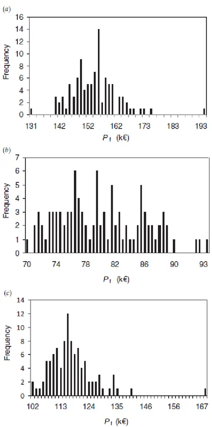
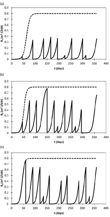
The distribution of solutions obtained for each scenario is summarized in Figure 5. The histograms indicate that a range of local optima exists, with the width of the range of solutions varying for each scenario: The range for Scenario A is 62 k€ whereas that for Scenario B is 23 k€. The optimal cleaning schedule obtained for each scenario, corresponding to the best local solution found with the multistart approach, is presented in Table 4. All three types of cleaning are performed and the units are cleaned regularly, but the distribution of types is not random. Unit 1 is only cleaned by water flushing or chemical action, and never by chemical cleaning and disinfection. The penalty for taking this larger duty unit off-line for 5 days is not matched by its performance afterward. This is illustrated by the individual Rf-t plots in Figure 6, where the fouling resistance in unit 1 does not exceed Rf∞/2. Units 2 and 3, in contrast, are cleaned by water flush or with chemicals and disinfectant. The number of cleaning actions over the year is large (28), with several intervals seeing two cleaning actions. Most of the cleaning actions are water flushes, which are attractive owing to the absence of downtime for cleaning more than compensating for the lack of an induction period subsequently.

In Scenario B the exchangers experience a reduced extent of fouling and the fouling penalty for the worst case (no cleaning) is now 120 k€. The lower Rf∞value results in smaller heat losses and reduced incentive to clean: The number of cleans is reduced to 13, giving an optimal cleaning cost of 70 k€, which is still a substantial saving. The schedule in Table 4 shows only chemical cleaning (no water flushes) for unit 1 and noticeably fewer water flushes (and only one disinfection) for units 2 and 3.

Reducing the rate of fouling in Scenario C (less rapid fouling) does not change the worst-case penalty significantly from the base case because the Rf values reach their asymptotic values relatively early. There are more cleaning actions than Scenario B (18 actions) and a noticeable change in the scheduling pattern, as there are now two chemical cleans plus disinfection. Water flushing is still common, but much less frequent than the base case (9 vs. 21 mentioned earlier).

The preceding results demonstrate that the particular features associated with biofouling, namely, the existence of a fouling induction period and asymptotic fouling, can be handled by the fouling model formulation described earlier. The fouling parameters used in the scenarios are based loosely on those reported in reference 24. Scenario B represents a process change that reduces Rf∞, such as operating at higher flow velocities to increase the shear stress acting on the biofilm [26], reducing the nutrient load [27], or manipulating surface adhesion [28]. Scenario C represents a process change that decreases the rate, such as reducing the level of nutrients present in the water or changing the temperature, which affects both oxygen solubility and bacterial growth rates [1]. The scheduling model can be used to quantify the benefit obtained from such a process modification and therefore to determine the return on any capital expenditure associated with

implementing that measure.

Application and Extension

The case-study results demonstrate that the mathematical formulation gives tractable results in a reasonable time scale, such that the approach could be applied to schedule cleaning on plants in real time. Ideally, the fouling growth rate model (Eq. (3)) would be linked to a biofilm monitoring system so that parameters kf and Rf,∞ can be identified and refined in an adaptive fashion. Several methods are available for biofilm monitoring [29], but the estimation of the thermal fouling resistance is very convenient for heat exchanger equipment [20]. Furthermore, plant monitoring data could be correlated against the cleaning performance of different methods for specifed biofilm ages (or formation conditions) and this information could be used to predict the b and tI parameters. Online monitoring can also enable determination of the cleaning endpoint [30], and again this historical information can be used to improve the model.

An important facet of biofilm behavior that is commonly associated with biofilm cleaning/disinfection but that is not considered in the model presented here is the development of resistance to antimicrobial agents. Mah and O’Toole [31] reported that biofilm cells can be up to 1000 times more resistant than cells grown in suspension; this resistance can either be intrinsic or acquired [32]. Intrinsic resistance explains phenomena like reduced penetration of antimicrobials due to diffusion limitations [31], degradation of the antimicrobials by specific enzymes [32], or the existence of naturally resistant forms, such as spore formers [33]. Acquired resistance is commonly obtained through mutation or acquisition of genetic material from plasmids or transponsons [32]. Some features of the intrinsic resistance (such as reduced penetration of the agent) may promote the formation of a concentration gradient inside the biofilm where cells are exposed to sublethal concentrations of that agent, thereby facilitating acquired resistance events [33].

Once a certain antimicrobial agent is found to be active against a particular organism, the effects of intrinsic resistance can often be circumvented by manipulation of the operating conditions used during treatment, such as reagent concentration, contact time, temperature, and turbulence of the cleaning/disinfection solution [20]. The effectiveness of a disinfection step can decrease between successive runs, and this has been attributed to acquired resistance [32]. An effective countermeasure is to change the disinfection protocol periodically. The alternative disinfection protocols (usually employing a different antimicrobial) are likely to have different associated costs and operating conditions (such as contact time).

Acquired resistance and changing effectiveness were not included in the formulation presented here but can be readily implemented by extending the choice of cleaning methods to have two disinfection steps. The constraint set for the optimization problem would then include a statement limiting the maximum number of times each disinfection step could be applied in succession, as well as modifying tI and b parameters to include changes arising from acquired resistance. Similarly, the maxi- mum time period over which a particular step should be applied can be set as a constraint.

CONCLUSIONS

A mathematical formulation for the problem of optimizing cleaning schedules to heat exchangers and networks subject to biofouling, which can exhibit sizeable induction periods, has been developed. The formulation includes, for the first time in this field, considerations of three different cleaning mechanisms with varying cost and effectiveness, which also determine the subsequent fouling behavior. Solutions can be obtained in reasonable time scales, and a case-study network is used to demonstrate the versatility of the approach and the scope for exploring the impact of different fouling mitigation strategies. The overall savings that can be attained by using this approach can be significant, and the tool can also be used to evaluate process changes involving substantial capital costs. Potential modifications to handle biofilm behavior such as aging and biocide resistance have been discussed.

FUNDING

Financial support for Thomas Pogiatzis from the Onassis Foundation and the Cambridge European Trust is gratefully acknowledged, as is permission from Professor L. Shi at Tsinghua University to present the data in Figure 1. Luciana Calheiros is gratefully acknowledged for her assistance in the preparation of this paper.

NOMENCLATURE

A heat transfer area, m2

b induction period reduction factor

Ck,i cleaning action cost, method k, unit i, €/clean f e energy cost, € W−1 day−1

i identifier, heat exchanger j indentifier, time interval

kf fouling rate parameter, m2 K J−1

MINLP multiple-integer nonlinear programming nu number of units Pf total cost of fouling, €

Q heat transfer duty, W

Qclean heat transfer duty, clean condition, W Rf fouling resistance, m2 K W−1

Rf,∞ asymptotic fouling resistance, m2 K W−1

T temperature, K

Tin temperature, inlet condition, K t time, s

tc downtime, chemical cleaning, s td downtime, disinfection, s t∗ elapsed time [Equation (3)], s

+

tH operating horizon length, s tI induction period length, s tL leap time, s

t0∗ fouling starting point, s

U _{overall heat transfer coefficient, W m2 K−1}

Uclean overall heat transfer coefficient, clean condition, W m2 K−1 W heat capacity flow rate, W K−1

yk,i cleaning decision variable, method k, unit i

Subscripts

d chemical cleaning disinfection c chemical cleaning

fl flush cleaning h hot stream

w cooling water stream

REFERENCES

1. Bott, T. R., Biological Growth on Heat Exchanger Sur- faces, in Fouling of Heat Exchangers, ed. T. R. Bott, Elsevier, Amsterdam, The Netherlands, pp. 223–262, 1995. 2. Mu¨ller-Steinhagen, H., and Zettler, H. U., Heat Exchanger Fouling: Mitigation and

Cleaning Technologies, Publico Publications, Essen, Germany, 2000.

3. Ishiyama, E. M., Paterson, W. R., and Wilson, D. I., Plat- form for Techno-Economic Analysis of Fouling Mitigation Options in Refinery Preheat Trains, Energy Fuels, vol. 23, pp. 1323–1337, 2009.

4. Lavaja, J. H., and Bagajewicz, M. J., On a New MILP Model for the Planning of Heat-Exchanger Network Cleaning, Industrial & Engineering Chemical Research, vol. 43, pp. 3924–3938, 2004.

5. Rodriguez, C., and Smith, R., Optimization of Operating Conditions for Mitigating Fouling in Heat Exchanger Net- works, Chemical Engineering Research and Design, vol. 85, pp. 839–851, 2007.

6. Sma¨ıli, F., Vassiliadis, V. S., and Wilson, D. I., Long-Term Scheduling of Cleaning of Heat Exchanger Networks—Comparison of Outer Approximation-Based Solutions With a Backtracking Threshold Accepting Algorithm, Chemical Engineering Research and Design, vol. 80, pp. 561–578, 2002.

7. Napoles-Rivera, F., Bin-Mahfouz, A., Jimenez-Gutierrez, A., El-Halwagi, M. M., and Ponce-Ortega, J. M., An MINLP Model for Biofouling Control in Seawater-Cooled Facilities, Computers & Chemical Engineering, vol. 37, pp. 163–171, 2012.

8. Simo˜es, M., Simo˜es, L. C., and Vieira, M. J., A Re- view of Current and Emergent Biofilm Control Strategies, LWT—Food Science and Technology, vol. 43, pp. 573–583,

9. Sommer, P., Martin-Rouas, C., and Mettler, E., Influence of the Adherent Population Level on Biofilm Population, Structure and Resistance to Chlorination, Food Microbiology, vol. 16, pp. 503–515, 1999.

10. Ishiyama, E. M., Paterson, W. R., and Wilson, D. I., Optimum Cleaning Cycles for Heat Transfer Equipment Under going Fouling and Ageing, Chemical Engineering Science, vol. 66, pp. 604–612, 2011.

11. Pogiatzis, T., Ishiyama, E. M., Paterson, W. R., Vassiliadis, V. S., and Wilson, D. I., Identifying Optimal Cleaning Cycles for Heat Exchangers Subject to Fouling and Ageing, Applied Energy, vol. 89, pp. 60–66, 2012.

12. Yang, Q., Wilson, D. I., Chen, X. D., and Shi, L., Experimental Investigation of Interactions Between the Temperature Field and Biofouling in a Synthetic Treated Sewage Stream, Biofouling, vol. 29, pp. 513–523, 2013.

13. Brooks, J. D., and Flint, S. H., Biofilms in the Food Indus- try: Problems and Potential Solutions, International Journal of Food Science & Technology, vol. 43, pp. 2163–2176, 2008.

14. Wilson, D. I., Challenges in Cleaning: Recent Developments and Future Prospects, Heat Transfer Engineering, vol. 26, pp. 51–59, 2003.

15. Flemming, H. C., Biofouling in Water Systems—Cases, Causes and Countermeasures, Applied Microbiology and Biotechnology, vol. 59, pp. 629–640, 2002.

16. Pogiatzis, T. A., Wilson, D. I., and Vassiliadis, V. S., Scheduling the Cleaning Actions for a Fouled Heat Ex- changer Subject to Ageing: MINLP Formulation, Computers & Chemical Engineering, vol. 39, pp. 179–185, 2012.

17. Abreu, A. C., Tavares, R. R., Borges, A., Mergulha˜o, F. and Simo˜es, M., Current and Emergent Strategies for Disinfection of Hospital Environments, Journal of Antimicrobial Chemotherapy, vol. 68, no. 12, pp. 2718–2732, 2013.

18. Ahimou, F., Semmens, M. J., Haugstad, G. and Novak, P. J., Effect of Protein, Polysaccharide, and Oxygen Concentration Profiles on Biofilm Cohesiveness, Applied Environ- mental Microbiology, vol. 73, pp. 2905–2910, 2007.

19. Epstein, A.K., Pokroy, B., Seminara, A., and Aizenberg, J., Bacterial Biofilm Shows Persistent Resistance to liquid Wetting and Gas Penetration, Proceedings of the National Academy of Sciences, USA, vol. 108, pp. 995–1000, 2011.

20. Marchand, S., De Block, J., De Jonghe, V., Coorevits, A., Heyndrickx, M., and Herman, L., Biofilm Formation in Milk Production and Processing Environments; Influence on Milk Quality and Safety, Comprehensive Reviews in Food Science and Food Safety, vol. 11, pp. 133–147, 2012.

21. Hewitt, G. F., Shires, G. L., and Bott, T. R., Process Heat Transfer, CRC Press, Boca Raton, FL, 1994.

22. Benders, J. F., Partitioning Procedures for Solving Mixed- Variables Programming Problems, Numerische Mathematik, vol. 4, pp. 238–252, 1962.

23. Geoffrion, A. M., Generalized Benders Decomposition, Journal of Optimization Theory and Applications, vol. 10, pp. 237–260, 1972.

24. Nebot, E., Casanueva, J.F., Casanueva, T., and Sales, D., Model for Fouling Deposition on Power Plant Steam Condensers Cooled With Seawater: Effect of Water Velocity and Tube Material, International Journal of Heat and Mass Transfer, vol. 50, pp. 3351–3358, 2007.

Redwood City, CA, 1992.

26. Moreira, J. M., Teodosio, J. S., Silva, F. C., Simo˜es, M., Melo, L. F., and Mergulha˜o, F. J., Influence of Flow Rate Variation on the Development of Escherichia coli Biofilms, Bioprocess and Biosystems Engineering, vol. 36, pp. 1787–1796, 2013.

27. Moreira, J. M. R., Gomes, L. C., Araujo, J. D. P., Miranda, J. M., Simo˜es, M., and Melo, L. F., The Effect of Glucose Concentration and Shaking Conditions on Escherichia coli Biofilm Formation in Microtiter Plates, Chemical Engeering Science, vol. 94, pp. 192– 199, 2013.

28. Rosmaninho, R., Santos, O., Nylander, T., Paulsson, M., Beuf, M., and Benezech, T., Modified Stainless Steel Sur- faces Targeted to Reduce Fouling—Evaluation of Fouling by Milk Components, Journal of Food Engineering, vol. 80, pp. 1176–1187, 2007. 29. Janknecht, P., and Melo, L. F., Online Biofilm Monitoring, Reviews in Environmental

Science and Bio/Technology, vol. 2, pp. 269–283, 2003.

30. Pereira, A., Mendes, J., and Melo, L. F., Using Nanovibrations to Monitor Biofouling, Biotechnology and Bioengineering, vol. 99, pp. 1407–1415, 2008.

31. Mah, T. F. C., and O’Toole, G. A., Mechanisms of Biofilm Resistance to Antimicrobial Agents, Trends in Microbiology, vol. 9, pp. 34–39, 2001.

32. McDonnell, G., and Russell, A. D., Antiseptics and Disinfectants: Activity, Action, and Resistance, Clinical Micro- biology Reviews, vol. 12, pp. 147–179, 1999.

33. Stewart, P. S., Mechanisms of Antibiotic Resistance in Bacterial Biofilms, International Journal of Medical Microbiology, vol. 292, pp. 107–113, 2002.

Figure 1 Fouling caused by mixed biofilm growth in an experimental heat exchanger processing treated sewage sludge. Dashed vertical lines separate the stages in biofouling. Data reproduced from [12].

Figure 2 Schematic of biofouling behavior (a) following different cleaning actions; (b) sigmoidal growth model of [24] employed in simulations, showing “leap” times.

Figure 3 Subdiscretization of time intervals. Flushing is assumed to take negligible process time.

Figure 4 Case study heat exchanger network showing cold stream temperatures under clean conditions. Solid line, cooling water; dashed lines, hot process streams.

Figure 5 Distribution of solutions generated by the GBD algorithm for 100 random starting points. (a) Scenario A; (b) Scenario B; (c) Scenario C.

Figure 6 Individual fouling profiles for each unit for optimal schedule, Scenario A. Dashed line shows profile in absence of cleaning for (a) unit 1; (b) unit 2; and (c) unit 3.

Table 4 Optimized cleaning schedules for case study scenarios: Modes: open circles, water flush (f); gray circles, chemical cleaning (c); black circles, chemical cleaning and disinfection (d), with U the heat exchanger identifier