MULTICRITERIA DECISION AID APPLICATION TO A STUDENT SELECTION PROBLEM
Juan Carlos Leyva López Departamento de Posgrado Universidad de Occidente Sinaloa – México [email protected]
Recebido em 01/2004; aceito em 12/2004 após 1 revisão Received January 2004; accepted December 2004 after one revision
Abstract
The selection of students is a complex decision making process, in which multiple selection criteria often need to be considered and where subjectiveness and imprecision are usually present, resulting that fuzzy and imprecise data should be used. This paper formulates the student selection process as a multicriteria decision analysis problem, concretely as a ranking problem, by using the ELECTRE III methodology to construct a fuzzy outranking relation, and then a genetic algorithm to exploit it and to obtain a ranking in decreasing order of preference. An empirical study of a real selection problem in the Universidad de Occidente in Mexico is presented. After performing calculations and obtaining the final ranking of compared alternatives, a sensitivity analysis was carried out. The study was supported with a new decision aid system for rank a finite set of multicriteria alternatives.
Keywords: multicriteria decision analysis; ranking problem; genetic algorithms; student
1. Introduction
Selecting students from competing applicants is a complex decision making process, which often requires a comprehensive evaluation of the applicant’s performance. Multiple selection criteria should be simultaneously considered, and subjective assessments are usually present, resulting in fuzzy and imprecise data.
Statistical procedures, such as discriminant analysis and regression analysis are traditionally used for predicting the potential academic success of the applicant (Graham, 1991). The predictive validity study may help make admission or selection procedures more efficient
and effective (Powers & Lehman, 1983; Dobson et al., 1999; Lievens & Coetsier, 2002).
However, the selection criteria used in higher education admission processes varies widely among programs and no consistent conclusions can be reached on the predictive values of these criteria (Wilson, 1999). This may partly be due to the fact that the predictive validity of the selection instruments is not in itself sufficient for an assessment of the validity of a selection, although it can be a critical factor (Wolming, 1999). In this paper, prediction is not the stated purpose for the student selection problem. The selection of applicants is made on the grounds of the candidates’ merits (performance evaluation) assessed by an interview process and his/her academic background, based on a given set of criteria in accordance with the requirements of the academic program of Master in Science. The artificial neural networks have also attracted the attention the last years (Flitman, 1997). However, the
effectiveness of these methods is sometimes questioned (Hardgrave et al., 1994), due to the
sophistication of the decision process, the rough assumptions required, and the level of accuracy achieved. They are, in particular, unable to adequately handle the subjectiveness and imprecision of the decision process and often impose a high cognitive effort on the decision maker (DM).
Alternatively, multicriteria analysis (MA) is widely used for selecting or ranking alternatives in relation to multiple criteria (Roy, 1996; Vanderpooten, 1990). In line with the multi-dimensional characteristics of the student selection process, MA provides an effective framework for solving the problem and, particularly, the approach based on fuzzy outranking relations, is adequate for dealing with situations in which imprecision and subjectiveness are
present (Rogers et al., 2000).
The application of fuzzy set theory in MA provides an effective means for modeling the subjectiveness and imprecision (Fodor & Roubens, 1994). When the Decision Maker is a
group of experts, Carlsson et al. (1997) illustrate the applicability of Ordered Weighted
the explicit global model of preferences could happen. In outranking methods, we can distinguish two phases: aggregation and exploitation. The aggregation process corresponds to the operation, which transforms the marginal evaluations of separate criteria into a global outranking relation between every pair of alternatives, which is generally not transitive nor complete. The exploitation process deals with the outranking relation in order to clarify the decision through a partial or total preordering reflecting some of the irreducible indifferences and incomparabilities (Fodor & Roubens, 1994).
To some extent fuzzy relations offer a compromise between value functions and preference relations; their power of expressiveness is far beyond the one of value functions since they are good models for such phenomena as non-transitivity and incomparability. ELECTRE III, PROMETHEE and other methods for decision aid (e.g. Roy, 1990; Fodor & Roubens, 1994) build and exploit a fuzzy outranking relation.
Let A be the set of alternatives or potential actions and let us consider a fuzzy outranking
relation SA
σ
defined on A X A; this means that we associate with each ordered pair (a, b) a
real number σ (a, b) (0≤ σ(a, b) ≤ 1) reflecting the degree of strength of the arguments
favoring the crisp outranking aSb. The exploitation phase transforms the global information
included in SA
σ
into a global ranking of the elements of A. Usually; three different ways are
used (Fodor & Roubens, 1994):
a: transform SA
σ
into another valued relation R which presents some interesting property needed for ranking purposes, i.e. transitivity,
b: determine a crisp binary relation close to SA
σ
, which presents crisp properties needed for ordering,
c: use a ranking method to obtain a score function.
Point a includes the process of finding the transitive closure or the intersection of traces. Point c is most commonly used in classical procedures like ELECTRE III and PROMETHEE. But the main difficult consists in finding reasonable ways of dealing with the intransitivities without losing too much of the contents of the outranking relation. In this
sense, the methods included in points a and b lose information coming from SA
σ when exploit a not so close transitive valued relation R, or a crisp binary relation with desirable properties for ranking purposes. On the other hand, the methods based in score functions do not perform well in presence of irrelevant alternatives or in case of complex graphs with many circuits. Non-rational situations could happen when the prescription is constructed.
Most significant is the following: Suppose that a and b are two actions such that σ (a, b) ≥λ
and σ (b, a) ≤λ-β (β>0); if λ≥c and β≥t (c and t representing consensus and threshold levels
respectively), we should accept that “a outranks b” (a Sλb) and “b does not outrank a”
(b nSλa); in this case the global preference model captured in outranking relation is giving a
presumed preference favoring a. However, a score function or other similar method (based
on flow of outranking or “distillation” process) could lead to a final ordering in which b is
In this paper, is formulated the student selection process as a MA problem, and is used a fuzzy MA approach for solving a real student selection problem at the Master in Management Information Systems (MMIS) of the Universidad de Occidente (U de O) in Mexico. The ELECTRE III – Genetic Algorithm approach can effectively calculate the overall performance of individual applicants, construct an aggregation model of preferences and exploit it to recommend to the DM a ranking of the applicants.
Section 2 describes the ELECTRE III method and the genetic algorithm, followed in Section 3 by an explanation of the student selection situation faced by the MMIS and, also in this section, is provided an empirical study to illustrate, one more time, the applicability of the approach. In Section 4, is carried out a sensitivity analysis of the final result. On these backgrounds, in Section 5 are presented the results and a brief discussion of the selection process. Finally in Section 6 are presented the conclusions.
2. The (ELECTRE III – Genetic Algorithm) Methodology
2.1 The ELECTRE method
As part of a philosophy of decision aid, ELECTRE (in its various forms) was conceived by Bernard Roy (1990) in response to deficiencies of existing decision making solution methods. Roy’s philosophy of decision aid is well exposed in Roy (1996) (see also Roy (1990) and Vanderpooten (1990) for basic introductions to these methods); moreover, of the different versions of ELECTRE which have been (I, II, III, IV, IS and TRI), only is used the method specifically referred to as ELECTRE III. All methods are based on the same fundamental concepts, as explained subsequently, but they differ both operationally and according to the type of decision problem. Specifically, ELECTRE I is designed for selection problems, ELECTRE TRI for assignment problems and ELECTRE II, III, and IV for ranking problems. ELECTRE II is an old version; ELECTRE III is used when it is possible and desirable to builds fuzzy outranking relationships and quantifies the relative importance of criteria and ELECTRE IV when this quantification is not possible (Roy & Bouyssou, 1993).
A number of factors influenced the specific selection of the ELECTRE III method for the Postgraduate student selection problem. Firstly, in Leyva (2000) is presented a genetic algorithm to exploit a fuzzy outranking relation and is interesting to show, one more time, and with a real world application the functionality between the pair (ELECTRE III, Genetic algorithms). Secondly, ELECTRE was originally developed by Roy to incorporate the fuzzy (imprecise and uncertain) nature of decision-making, by using thresholds of indifference and preference. This feature is appropriate for solving this problem. A further feature of ELECTRE, which distinguishes it from many multiple criteria solution methods, is that it is fundamentally non-compensatory. This means, in particular that, good scores on other criteria cannot compensate a very bad score on a criterion. Another feature is that ELECTRE models allow incomparability. Incomparability, which should not be confused with indifference, occurs
between some alternatives a and b when there is no clear evidence in favour of some kind of
preference or indifference. Finally, the choice of ELECTRE III was also influenced by
successful applications of the approach (for example: Roger et al., 2000; Hokkanen &
Salminen, 1997; Al-Kloub et al., 1997; Georgopoulou, 1997; Roger & Bruen, 1998).
Two important concepts that underline the ELECTRE approach, thresholds and outranking,
of alternatives A. Traditional preference modeling assumes the following two relations
holded for two alternatives ( ,a b)∈A:
a is pref a is indiffe
a is preferred is indifferen
( ;
ongly pref akly pref
fferent to b
( ) ( ( ) ( ) ( ) ) ( ) ⇔ > ⇔ =
aPb erred to b g a g b
aIb rent to b g a g b
In contrast, ELECTRE methods introduce the concept of an indifference threshold, q, and
then the preference relations are redefined as follows:
( ) ( )
( ) ( )
( ) ( )
⇔ > +
⇔ − ≤
aPb to b g a g b q
aIb a t to b g a g b q
While the introduction of this threshold goes some way toward incorporating how a decision maker actually does feel about realistic comparisons, a problem remains. There is a point at which a decision maker changes from indifference to strict preference. Conceptually, there is a good reason to introduce a buffer zone between indifference and strict preference, an intermediary zone where a decision maker hesitates between preference and indifference.
This zone of hesitation is referred to as a weak preference; it is also a binary relation like P
and I above, and is modeled by introducing a preference threshold, p. Thus, we have a double
threshold model, with an additional binary relation Q that measures weak preference. That is:
( ) ( )
( ) (
) ( ) (
⇔ − >
⇔ < − ≤
⇔ − ≤
aPb a is str erred to b g a g b p
aQb a is we erred to b q g a g b p
aIb a is indi and b to a g a g b q ( )
) ( )
)
The choice of thresholds intimately affects whether a particular binary relation holds. While the choice of appropriate threshold is not easy, in most realistic decision making situations
there are good reasons for choosing non-zero values for p and q.
Note that we have only considered the simple case where thresholds p and q are constants, as
opposed to being functions of the value of the criteria; that is, the case of variable thresholds. While this simplification of using constant thresholds aids the exposition of the ELECTRE method, it may be worth using variable thresholds, in case where the criterion having larger values may lead to larger indifference and preference thresholds.
Using thresholds, the ELECTRE method seeks to build an outranking relation S. aSb means
that according to the global model of DM preferences, there are good reasons to consider that
“a is at least as good as b” or “a is not worse than b.” Each pair of alternatives a and b is then
tested in order to check if the assertion aSb is valid or not. This give rise to one of the
following four situations:
aSb and not(bSa); not(aSb) and bSa; aSb and bSa; not(aSb) and not(bSa).
Observe that the third situation corresponds to indifference, while the fourth corresponds to incomparability.
The test to accept the assertion aSb is implemented using two principles:
i) A concordance principle which requires that a majority of criteria, after considering their relative importance, is in favor of the assertion – the majority principle, and ii) A non-discordance principle, which requires that within the minority of criteria,
The operational implementation of these two principles is now discussed, assuming that all criteria are to be maximized. We first consider the outranking relation defined for each of the r criteria; that is,
j
aS b Means that “a is at least as good as b with respect to the jth criterion,” j=1,2,…,r
The jth criterion is in concordance with the assertion aSb if and only if aSjb. That is, if
( )≥ ( )−
j j j
g a g b q . Thus, even if g aj( ) is less than g bj( ) by an amount up to qj, it does
not contravene the assertion aS bj and therefore is in concordance.
The jth criterion is in discordance with the assertion aSb if and only if bPja. That is, if
( )≥ ( )+
j j j
g b g a p . That is, if b is strictly preferred to a for criterion j, then it is clearly not
in concordance with the assertion that aSb.
With these concepts it is now possible to measure the strength of the assertion aSb. The first
step is to develop a measure of concordance, as contained in the concordance index C (a, b),
for every pair of alternatives ( , )a b ∈A. Let kj be the importance coefficient or weight for
criterion j. We define a valued outranking relation as follows:
1 1
1
( , ) ( , ),
= =
=
∑
r j j =∑
rj j
C a b k c a b where k k
k j (1)
Where
1, ( ) ( )
( , ) 0, ( ) ( ) , 1, 2,...,
( ) ( ) ,
j j j
j j j j
j j j
j j
if g a q g b
c a b if g a p g b j r
p g a g b
otherwise
p q
+ ≥
= + ≤
+ −
−
=
Thresholds and weights represent subjective input provided by the decision maker. Weights used in the non-compensatory ELECTRE model are quite different from weights used in others, compensatory, decision modeling approaches such as the decision analytic approach (SMART) of Edwards (1997). In the decision analytic models, for example, weights are substitution rates and assess relative preference among criteria. Weights in ELECTRE are “coefficients of importance” and, as Vincke (1992) points out, they are like votes given to
each of the criterion “candidates.” Roger et al. (2000) review existing weighting schemes for
ELECTRE and provide a useful discussion of the weighting concept in ELECTRE. Care also needs to be taken in determining threshold values, which must relate specifically to each criterion and reflect the preferences of a decision maker. Procedures for choosing appropriate threshold values are addressed by Roger & Bruen (1998).
Thus far, no consideration has been given to the discordance principle. In the concordance index, we have, in a manner of speaking, a measure of the extent to which we are in harmony
with the assertion that a is at least as good as b. But what disconfirming or “disharmonious”
evidence do we have? In other words, is there any discordance associated with the
defined. The veto threshold vj
>
, allows for the possibility of aSb to be refused totally if, for
any one criterion j, g bj( ) g aj( )+vj. The discordance index for each criterion j, d a
is calculated as:
( , ) j b
0, ( ) ( )
( , ) 1, ( ) ( ) , 1, 2,...,
( ) ( ) , + ≥ = + ≤ − − −
j j j
j j j j
j j j
j j
if g a p g b
d a b if g a v g b j r
g b g a p
otherwise
v p
= (2)
For each pair of alternatives ( , )a b ∈A, there are now a concordance and a discordance
measure. The final step in the model building phase is to combine these two measures to produce a measure of the degree of outranking; that is, a credibility index which assesses the strength of the assertion that “a is at least as good as b.” The credibility degree for each pair
is defined as:
( , )a b ∈A
( , )
( , ), ( , ) ( , )
1 ( , )
( , ) ( , )
1 ( , ) ( , ) ( , ) ( , ) ∈ ≤ ∀ − = − • >
∏
j jj J a b
j
C a b if d a b C a b j
d a b
S a b where J a b is the set of criteria
C a b C a b
such that d a b C a b
(3)
This formula assumes that, if the strength of the concordance exceeds that of the discordance, then the concordance value should not be modified. Otherwise, we are forced to question the
assertion that aSb and modify C (a,b) according to the above equation. If the discordance is
1.0 for any ( , )a b ∈A and any criterion j, then we have no confidence that aSb; therefore,
S (a,b) = 0.0. The credibility matrix for this application is explained in Table 6.
This concludes the construction of the outranking model. The next step in the outranking approach is to exploit the model and produce a ranking of alternatives from the fuzzy outranking relation. Our approach for exploitation is using a genetic algorithm-based heuristic method (Leyva & Fernandez, 1999), which is explained, briefly in the next section.
2.2 The Genetic Algorithm for Deriving Final Ranking
In this section are explained some elements of the genetic algorithm which allows us to exploit a known fuzzy outranking relation with the purpose of constructing a prescription for the multi criteria ranking problem.
2.2.1 Encoding the solutions and the fitness function
alphabet where n is the number of actions into the decision problem. In such representation, each action is coded into n-ary form. Actions are then linked together to produce one long
n-ary string or chromosome. An action coded with aki value in the i-th entry of the string
means that the action coded with aki value is ranking in the i-th place of the ordering and
aki is preferred to akj if i < j, where aki∈ A = {a1, a2, …, an}, i=1, 2, …, n, and
[k1, k2, …, kn] is a permutation of [1, 2, …, n]. Each individual is associated with a number
λ (0 ≤λ≤ 1), which will be connected with the credibility level of a crisp outranking defined
on the set of genes. The fitness of an individual with credibility level λ is calculated
according to a given fitness function. The approach for defining individual’s fitness involves
separating the single fitness measure into two, one is called fitness and the other is called
unfitness. We chose the fitness function f of an individual p with credibility level λ as follows:
Let p = ak1ak2 … akn be the schematic representation of an individual’s chromosome and
suppose that given aki and akj, two actions such that σ (aki, akj) ≥λ and σ (akj, aki) ≤
λ-β (β>0, representing a threshold level), we accept that “aki outranks akj” (aki Sλakj)
and “akj does not outrank aki” (akj nSλ aki). In this case, into the crisp outranking
relation generated by λ, SAλ, a presumed preference favoring aki, holds. Then:
f(p) ={ (aki, akj) :aki nS akj and akj nS aki i = 1,2, ..., n-1, j = 2,3, ..., n, i<j }
where [k1, k2, ..., kn] is a permutation of [1,2,...,n].
f(p) is the number of incomparabilities between pairs of actions (aki, akj) into the
individual p = ak1ak2 … akn in the sense of the crisp relation SAλ. Note that the quality
of solution increases with decreasing fitness score.
The unfitness u of an individual p measures the amount of unfeasibility (in relative terms)
and we chose to define it as:
u(p) ={ (aki, akj) :aki S akj and akj nS aki; i = 1,2, ..., n, j = 1,2, ..., n, i>j }.
u(p)
is the number of preferences between actions into the individual p which are not
“well-ordered” in the sense of SAλ.
An individual P is feasible if u(p) = 0 and infeasible if u(p) > 0. Defining the unfitness
taking the zero minimum value if and only if the solution is feasible seems a natural
approach. Each individual p can then be represented by a triad of values f, u and λ.
We are interested in:
ii) individuals whose fitness function value is equal (or near) to zero. This objective improves the comparability of S on A.
iii) individuals whose credibility level λ is near to 1. This indicates us that the ordering
represented by the individual with credibility level λ is more trusty whenever the
fitness and unfitness function values are zero or near to zero. In practice, the
requirement connected to fitness function does not permit that λ values approach to 1
because in this case we could have many incomparable genes.
Then, we use a genetic search for solving the multiobjective optimization problem
Min u, f, Max λ
Rs , λ∈[0,1] λ≥λ0
Where Rs is a strict total order of A.
2.2.2 Crossover and mutation operators
The crossover operator takes genes from each parent string and “combines” them to create a child string. The main reason is that by creating new strings from fit parent strings, new and promising areas of the search space will be explored. Many crossover techniques exist in the literature (e.g. Ordoñez & Valenzuela, 1992), but, when working with ordinal (permutation) encoding, it is necessary to create both crossover and mutation operators that are specifics to this form of encoding. The main difficulty encountered when using non-standard representations is the design of a suitable crossover operator, which must combine relevant characteristics of the parent solutions into a valid offspring solution. In this paper we make use of the crossover operator UX2 (Union Crossover #2) first introduced in Poon & Carter (1995).
The mutation operator is applied to the child string generated after crossover operator is finished. It works by interchanging two pairs of randomly chosen genes (actions), at each iteration under certain rules, in an individual. Mutation is generally seen as a background operator, which provides a small amount of random search. It also helps to keep against loss of valuable genetic information by reintroducing information, which was lost due to premature convergence, and thereby, expanding the search space.
2.2.3 Parent selection method
Parent selection is the task of assigning reproductive opportunities to each individual in the population based on its relative fitness. A commonly used method is binary tournament selection. In a k-ary tournament selection, k individuals are chosen randomly from the population, and the most fitted individual is then allocated in a reproductive trial. In order to produce a child, two k-ary tournaments are held, each of which produces one parent string. These two parent strings are then combined to produce a child.
help the GA in finding feasible solutions. On the other hand, if we favor selection of less infeasible individuals, we might select individual, which are less fitted. Whilst feasibility
may improve, the solution quality could suffer. To avoid this, we developed a Complement
Selection (CS) method for selecting parents that attempts to improve comparability as well as feasibility.
The CS method is designed specifically for our problem and it takes into account the
credibility level λ of the candidate parents. In a complement selection, a parent Pi (Pj) is first
(second) selected using a k-ary tournament based on the unfitness (fitness) function and credibility level; the rule is as follow:
We selected the individual Pi (Pj) which has lowest unfitness (fitness) score and its
credibility level λPi(λPj) is greater than λP or λK, where λP is the average credibility level
of the population and λK is the average credibility level of the tournament. If i (j) is not
unique, then we select the individual with higher credibility level score. If there is not such i
(j) we tried the rule with the individual Pl, which has next lower unfitness (fitness) score;
continue until the rule is satisfied.
The logic here is that we would like the two parents together to cover as few amount of preference violations and incomparabilities between actions as possible, i.e. a low u(Pi) and
f(Pj)) with as high credibility level values λPi and λPj as possible.
2.2.4 Population replacement scheme
This GA part defines how new chromosomes will be put into the existing population. In this algorithm the current population is updated continuously during the mating process. After that the child has been produced through the GA operators, it will replace the “less fitted” member of the population. The average unfitness and/or fitness of the population will improve if the child solution has lower unfitness and fitness scores than those of the solutions being replaced. In this algorithm, every new offspring is replacing the worst chromosome in the population. We utilize the following approach in order to decide which is the worst individual in the population: Firstly we sort the population, in the present generation, by decreasing order of unfitness value – Criterion: If the unfitness value of the individual posed
in j place (u(Pr)) is less than the unfitness value of the individual posed in j-1 place (u(Ps)) or
if u(Pr) = u(Ps) and f(Pr) < f(Ps) then we interchange the individuals, otherwise we do not
interchange (in case of tie, the fitness value is used in order to decide); in this way last individual is the worst. Each time that we replace a new offspring by the worst individual, the new population is sorted with the same criterion.
3. Postgraduate Student Selection: A Mexican Case
This applicant ranking problem is, like many decision problems, challenging because there is no single criterion that adequately captures the performance of each applicant; in other words, it is a multicriteria problem.
study mode. It means that the student may have another activities like working as a full-time or part-time worker. As an important part of the selection process, the MMIS program needs to know and have a dedication agreement with each one of its students.
Until the past generation at MMIS, the selection process had been carried out in an ad hoc manner. DM (which in this case is a committee formed by postgrade academics) made its decisions mainly based on the academic performance of the applicants on an introductory course on Programming Language C/C++, the DM used also its experience, intuition and knowledge with the information available. A structured approach capable of producing consistent decision outcomes through adequately handling the inherent imprecision and subjectiveness is obviously desirable.
For the postgraduate student selection problem, the decision alternatives are clearly defined as each one of the applicants. Each applicant or alternative is characterized by her attributes, which are then related to the criteria.
3.1 Defining the criteria family
According to Bouyssou (1990) the criteria family should be legible (containing sufficiently small number of criteria), operational, exhaustive (containing all points of view), monotonic and non-redundant (each criterion should be counted only once). These rules provide a coherent criterion family.
In our approach, in order to define the criteria, the analyst worked close to the DM. He had in mind that selecting a qualified applicant could only be the first parameter in the planning procedure. A series of other parameters should be taken into account, being the most important:
• The size of the academic staff
• The experience gained in past selection processes
• The correspondence between the number of research projects and the number of
accepted applicant to the program
• The finance security
• The graduated index
• The developing program of the MMIS
• The existence of the necessary infrastructure
• Other national targets such as employment, scientific political, etc.
• The academic and social impacts in our environment
• The technical and financial risk.
Table 1 – Ranking criteria.
Label Criterion Purpose/scope of the criterion Measurable parameters
Max/ Min C1* Intelligence of
the applicant
It is a reflection of the applicant’s programming language and mathematical skills in problems solving. It depends on several factors such as homework, participation in class and the academic performance on programming language and mathematics based on a test.
General score on an introductory course.
Maximize
C2* Academic performance
It is a reflection of the applicant’s capability to successfully complete their studies. This is measured by the academic results of the applicant in their previous studies and the performance of the applicant in their interviews.
General score of the previous studies.
Maximize
C3* Time spent in studying
It ensures the availability of the applicant. It measures the number of hours by week that he/she will dedicate to study.
Maximize
C4* English proficiency
It guarantees the proficiency on a second language. It is assessed based on applicant’s documents like TOEFL certificate or the certificate drawn up by the Foreign Language Center of the U de O or on the result of an English test.
It measures the ability of the applicant to adequately use the English language. It is measured with a transformed score based in the scale 0-10.
Maximize
C5* Responsibility and performance
It guarantees some values in the applicant such as the applicant’s personality, attitude towards works, punctuality, presence, interest, homework etc.
Measures the DM’s subjective assessment with respect to several factors.
Maximize
C6 General knowledge test
It guarantees the minimum knowledge to gain admittance in the program.
Score of a general test. Maximize
Most criteria were decomposed into simpler and well-defined attribute measures, which were then combined to produce a score for each applicant for each criterion. The score for the intelligence criterion (C1), the academic performance criterion (C2), the English proficiency criterion (C4), and the responsibility performance criterion (C5) were scaled from 0 to 10, the time spent in studying (C3) was scaled from 0 to 50; the units of these criteria are not meaningful outside this case study. The actual scores for each criterion are defined by a number of attributes that together describe the performance of the applicant. For example, the intelligence introduced by a particular applicant may influence the grade on programming language and mathematical subjects. In each case, a logical o arithmetic formula is defined to produce the score for each criterion. This input, where each applicant is assessed across each criterion, produces a matrix of performances. Table 3, into the Subsection 3.2, provides the performance matrix, for twenty-one applicants and five criteria.
3.2 The real world application
The next instance of the ranking problem discusses an empirical study of the following real selection problem sufficiently described above.
identify the best possible candidates. After that, the DM saw many interested persons to enroll in the program, they finally accepted to compete for a place 21 applicants labeled in this application as A1, A2, …, A21. The study was supported with a new decision aid system for rank a finite set of multicriteria alternatives, developed by our working group and whose main window is presented in Figure 1.
Figure 1 – Main window of the software SADAGE.
The DM has made an adequately comprehensive description of each applicant available. For this application, the 5 following criteria and its scale are formulated in the Table 2.
Table 2 – Criteria and its scale.
Label 1 Label 2 Criterion Scale
C1 INT Intelligence 0-10
C2 AP Academic performance 0-10
C3 TSS Time spent in studying 0-50
C4 EP English proficiency 0-10
C5 RP Responsibility performance 0-10
As mentioned in Subsection 2.1, three are the main inputs of the ELECTRE method.
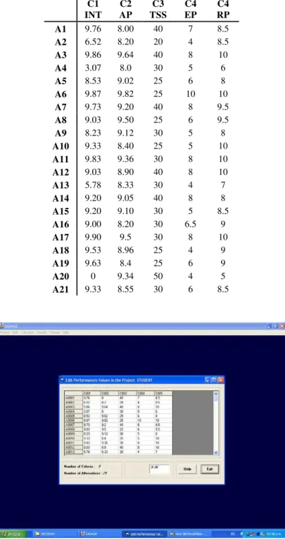
3.2.1 The performance matrix
Table 3 – Performances of the alternatives.
C1 INT
C2 AP
C3 TSS
C4 EP
C4 RP
A1 9.76 8.00 40 7 8.5
A2 6.52 8.20 20 4 8.5
A3 9.86 9.64 40 8 10
A4 3.07 8.0 30 5 6
A5 8.53 9.02 25 6 8
A6 9.87 9.82 25 10 10
A7 9.73 9.20 40 8 9.5
A8 9.03 9.50 25 6 9.5
A9 8.23 9.12 30 5 8
A10 9.33 8.40 25 5 10
A11 9.83 9.36 30 8 10
A12 9.03 8.90 40 8 10
A13 5.78 8.33 30 4 7
A14 9.20 9.05 40 8 8
A15 9.20 9.10 30 5 8.5
A16 9.00 8.20 30 6.5 9
A17 9.90 9.5 30 8 10
A18 9.53 8.96 25 4 9
A19 9.63 8.4 25 6 9
A20 0 9.34 50 4 5
A21 9.33 8.55 30 6 8.5
3.2.2 The thresholds
The DM was supported in the definition of its preferences and uncertainties through the q, p, and v thresholds for all criteria, with the following guidelines:
Agreeing with Rogers & Bruen (1998) we did not propose a specific relation between q and p values. As far as the veto threshold v is concerned, we suggested that veto should be the most important factor for the most important criteria. As a result, in the most important criteria (the ones with greater weight values) v should have been closer to p than in the case of the least important ones. In this way, we ensured that is difficult for a not important criterion to exercise veto against important criteria. It has been assumed that the thresholds
values shall be constant for all criteria (α=0). Thus, the thresholds value reflects the value of
β coefficient.
C1- Intelligence
This was the most important criterion. The DM wanted to accept mainly applicants
consistent with the MMIS objectives. As a result, the indifference threshold q was small,
with a value of 0.2 while the preference threshold was p=0.5. In a similar concept, v was only twice as p, since the DM did not want to accept an applicant not consistent with the MMIS objectives, in the place of a consistent one.
C2- Academic performance
In any case, academic performance of the applicant in their previous studies cannot help from being an important decision parameter. Alike criterion C1, the DM set q=0.2 and p=0.5. Considering that a distillation of applicants was made previously, veto was easy to happen requiring rather small differences. We set v=1.0.
C3- Time spent in studying
Since the program is offered as a part-time study mode, the DM wanted to assure a minimum dedication of applicant’s time. This criterion was allowed to have rather small indifference and weak preference zones, we set q=4 and p=9. However, considering the intrinsic subjectivity of this criterion, it could not easily exercise a veto. Threshold v was set to 40.
C4- English proficiency
English proficiency is ultimately an important decision factor. However, we set the veto threshold to 6, a rather high value, in order not to easily exclude from our short-list of applicants. q=1, p=1.5, v=6.0.
C5- Responsibility performance
Responsibility performance is of great value in the selection process. As a result q=0.5, p=1.0. However, in any case this is difficult to evaluate. As a result the veto threshold was rather high, v=7.0.
Table 4 – q, p, v threshold values.
Criterion q p v
C1. Intelligence 0.2 0.5 1.0
C2. Academic performance 0.2 0.5 1.0 C3. Time spent in studying 4 9 40 C4. English proficiency 1 1.5 6 C5. Responsibility performance 0.5 1.0 7.0
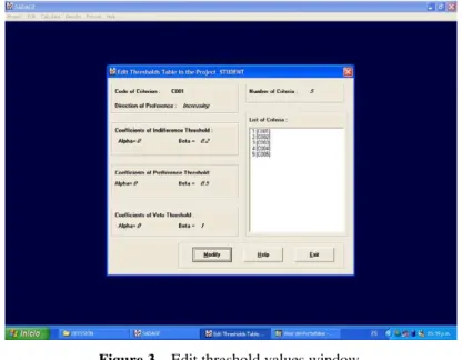
Figure 3 shown the threshold values of a criterion.
Figure 3 – Edit threshold values window.
3.2.3 The weights (relative importance of the criteria)
The DM was supported in the definition of the 5 criteria weights, as shown in Table 5. Personal
Construct Theory – PCT as suggested by Rogers et al. (2000) was used for the weight definition.
Table 5 – Criteria weights.
C1 C2 C3 C4 C5 RtC RtC +1 Weight Final
weight
C1 ---- X X X X 4 5 38.4 4
C2 ---- X X X 3 4 30.7 2.5
C3 ---- E X 1 2 15.3 1.5
C4 ---- E 0 1 7.7 1.0
C5 ---- 0 1 7.7 1.0
Total 13
3.3 Calculations and the final ranking
The input data used in calculations are the values presented in Table 3 (performances of the alternatives). All compared alternatives and criteria have been taken as the foundation for the calculation. Information about the preferences of the decision maker, namely, the values of
indifference, preference and veto thresholds for each criterion (defining α and β coefficients
for thresholds functions), and values of relative importance of criteria have been presented in Table 4 and Table 5. The decision maker’s experience constituted a basis for evaluation of the alternatives at hand, and was implemented by providing such information about the decision maker’s preferences, obligatory in the chosen computation method. It has been
assumed that the thresholds values shall be constant for all criteria (α=0). Thus, the threshold
value reflects the value of β coefficient. The values of relative importance of the criteria
indicate that what is most important for the decision maker is: the intelligence criterion and the academic performance.
The computation has been made on the input data (Table 3), and on the information about preferences of the decision maker (Table 4 and Table 5), using the ELECTRE III method.
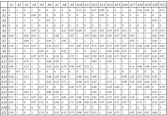
According to the additional information pointed out before, we applied ELECTRE III to construct a fuzzy outranking relation. Table 6 shows the credibility matrix obtained.
Table 6 – Credibility matrix.
A1 A2 A3 A4 A5 A6 A7 A8 A9 A10 A11 A12 A13 A14 A15 A16 A17 A18 A19 A20 A21 A1 1 1 0 1 0 0 0 0 0 0.73 0 0.37 0.89 0 0 1 0 0.24 0.83 0 0.75 A2 0 1 0 0.85 0 0 0 0 0 0 0 0 0.85 0 0 0 0 0 0 0 0 A3 1 1 1 1 1 0.9 1 1 1 1 1 1 1 1 1 1 1 1 1 0.85 1 A4 0 0 0 1 0 0 0 0 0 0 0 0 0 0 0 0 0 0 0 0 0 A5 0 1 0 0.97 1 0 0 0.27 0.97 0.40 0 0.25 0.97 0.35 0.57 0.51 0 0 0 0.75 0.53 A6 0.85 1 0.85 0.97 1 1 0.85 1 0.97 1 0.97 0.85 0.97 0.85 0.97 0.97 0.97 1 1 0.85 0.97 A7 1 1 0.80 1 1 0.65 1 0.92 1 1 1 1 1 1 1 1 0.92 1 1 0.85 1 A8 0.45 1 0.18 0.97 1 0.16 0.32 1 0.97 0.87 0.35 0.75 0.97 0.75 0.97 0.97 0.23 0.60 0.60 0.85 0.84 A9 0 1 0 1 0.87 0 0 0.22 1 0 0 0.12 1 0.03 0.09 0.31 0 0 0 0.83 0 A10 0.44 1 0 0.97 0.75 0 0.10 0 0.72 1 0.02 0.50 0.97 0.50 0.72 0.87 0 0.75 0.87 0.18 0.97 A11 0.85 1 0.78 1 1 0.68 0.85 1 1 1 1 0.85 1 0.85 1 1 1 1 1 0.85 1 A12 0.60 1 0.15 1 1 0.02 0.52 0.75 0.98 0.87 0.25 1 1 1 1 1 0.14 0.60 0.60 0.65 0.87 A13 0 0.5 0 1 0 0 0 0 0 0 0 0 1 0 0 0 0 0 0 0 0 A14 0.60 1 0.23 1 1 0.06 0.50 0.69 1 0.90 0.41 0.90 1 1 1 0.90 0.25 0.73 0.59 0.78 1 A15 0.35 1 0 1 1 0.02 0.22 0.73 1 0.90 0.35 0.65 1 0.75 1 0.90 0.16 0.83 0.69 0.82 1 A16 0.39 1 0 1 0.75 0 0 0 0.48 0.73 0 0.40 1 0.30 0.60 1 0 0.26 0.60 0 0.70 A17 0.85 1 0.85 1 1 0.80 0.85 1 1 1 1 0.85 1 0.85 1 1 1 1 1 0.85 1 A18 0.71 1 0.11 0.97 0.9 0 0.72 0.65 0.97 0.90 0.39 0.65 0.97 0.75 0.97 0.87 0.18 1 0.90 0.70 0.87 A19 0.85 1 0 0.97 0.75 0 0.40 0 0.72 0.90 0.09 0.40 0.97 0.50 0.72 0.97 0 0.75 1 0.18 0.97 A20 0 0 0 0 0 0 0 0 0 0 0 0 0 0 0 0 0 0 0 1 0 A21 0.54 1 0 1 0.78 0 0.10 0.19 0.75 0.90 0.07 0.53 1 0.50 0.75 1 0.02 0.83 0.87 0.60 1
The computation in the genetic algorithm was realized with the following parameters: 100 trials of the GA heuristic (each one with a different random seed) were generated. We worked with groups of 25 trials, which finished when {400, 350, 300, 300} populations had been generated. The population size was set to {55, 50, 40, 60}. The crossover probability was chosen {0.85, 0.75, 0.75, 0.70} and the mutation probability was {0.50, 0.60, 0.65, 0.50} respectively in each case. The final ranking obtained using the genetic algorithm is shown in Figure 4. Figure 5 illustrates part of the final ranking window.
Figure 4 shows part of the final ranking.
A6 ≻ A17 ≻ A7 ≻ A3 ≻ A11 ≻ A1 ≻ A8 ≻ A18 ≻ A14 ≻ A19 ≻ A21 ≻ A12 ≻ A15
≻ A16 ≻ A10 ≻ A9 ≻ A5 ≻ A2 ≻ A13 ≻ A20 ≻ A4
The credibility level was λ=0.7039.
Figure 4 – Final ranking.
Figure 5 – Final ranking window.
4. Sensitivity Analysis of the Final Result
In most cases, arriving at the final ordering accepted by the decision maker does not conclude the decision aiding process. The analyst can additionally propose to perform a sensitivity analysis. Examples of employing the sensitivity analysis have been presented also
in Briggs et al. (1990), Goicoechea et al. (1982) and Rios Insua & French (1991).
the form of the final result (the various methods use different parameters reflecting the decision making’s preferences). It is quite useful in the interpretation of results, which have been achieved at, in the course of modifying the values of the appropriate parameters reflecting the decision maker’s preferences, and in estimating the influence of the modifications on the final result. The decision maker has quoted some changes in values, which he accepts, with relation to the chosen parameters reflecting his preferences.
On such a basis, the range of sensitivity analysis has been defined, and it comprised the following:
• Taking into consideration the changes in values of relative importance (w) of criteria
for single criteria in the originally assumed arrangement of relative importance of values;
• Taking into consideration the changes in values of relative importance (w) of criteria
for a number of criteria at the same time which, as a result, generates a change of the whole arrangement of values of relative importance;
• Taking into consideration the changes of values for threshold functions: for the
thresholds of indifference (q), preference (p) and veto preference (v), for a single criterion;
• Taking into consideration the changes of values for thresholds functions: for the
thresholds of indifference (q), preference (p), and veto preference (v), for a number of criteria at the same time.
The results of the sensitivity analysis, which has been performed, depending on the range of shifting values of selected parameters of the decision maker preferences, have been presented in Table 7 (the arrangement of originally agreed upon input values for all parameters can be found in Table 4 and Table 5).
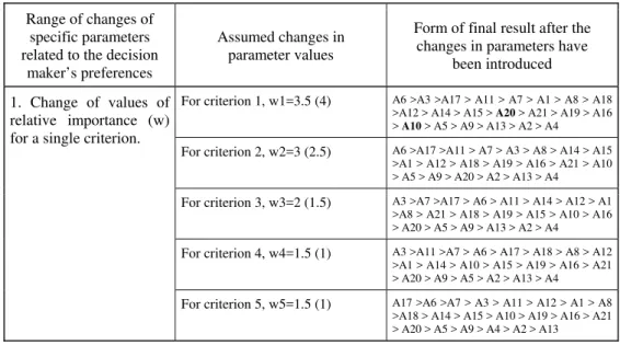
Table 7 – Presentation of the influence of changes in specific parameters and changes in values of chosen parameters on the form of the final result.
Range of changes of specific parameters related to the decision
maker’s preferences
Assumed changes in parameter values
Form of final result after the changes in parameters have
been introduced
For criterion 1, w1=3.5 (4) A6 >A3 >A17 > A11 > A7 > A1 > A8 > A18 >A12 > A14 > A15 > A20 > A21 > A19 > A16 > A10 > A5 > A9 > A13 > A2 > A4
For criterion 2, w2=3 (2.5) A6 >A17 >A11 > A7 > A3 > A8 > A14 > A15 >A1 > A12 > A18 > A19 > A16 > A21 > A10 > A5 > A9 > A20 > A2 > A13 > A4
For criterion 3, w3=2 (1.5) A3 >A7 >A17 > A6 > A11 > A14 > A12 > A1 >A8 > A21 > A18 > A19 > A15 > A10 > A16 > A20 > A5 > A9 > A13 > A2 > A4
For criterion 4, w4=1.5 (1) A3 >A11 >A7 > A6 > A17 > A18 > A8 > A12 >A1 > A14 > A10 > A15 > A19 > A16 > A21 > A20 > A9 > A5 > A2 > A13 > A4
1. Change of values of relative importance (w) for a single criterion.
For criterion 1, w1=3.5 (4) For criterion 2, w2=3 (2.5)
A17 >A1 >A3 > A6 > A7 > A11 > A12 > A18 >A8 > A14 > A21 > A15 > A19 > A20 > A16 > A10 > A9 > A5 > A13 > A2 > A4
For criterion 1, w1=3 (4) For criterion 4, w4=2 (1)
A3 >A6 >A11 > A17 > A7 > A12 > A1 > A8 >A18 > A19 > A14 > A15 > A10 > A20 > A21 > A9 > A16 > A5 > A2 > A13 > A4
For criterion 1, w1=3 (4) For criterion 5, w5=2 (1)
A3 >A6 >A7 > A11 > A17 > A12 > A8 > A18 >A15 > A19 > A1 > A10 > A14 > A21 > A20
> A5 > A9 > A2 > A13 > A16 > A4
For criterion 2, w2=2 (2.5) For criterion 3, w3=2 (1.5)
A6 >A17 >A7 > A11 > A3 > A18 > A1 > A8 >A12 > A14 > A20 > A15 > A19 > A10 > A21 > A16 > A2 > A5 > A9 > A13 > A4
For criterion 2, w2=2 (2.5) For criterion 4, w4=1.5 (1)
A6 >A7 >A3 > A17 > A11 > A1 > A12 > A8 >A14 > A15 > A19 > A21 > A18 > A10 > A20
> A16 > A9 > A5 > A2 > A13 > A4
2. Change of values of relative importance (w) for two or more criteria at the same time.
For criterion 3, w3=1 (1.5) For criterion 4, w4=1.5 (1)
A17 >A6 >A3 > A7 > A11 > A8 > A19 > A1 >A15 > A14 > A12 > A18 > A21 > A10 > A16 > A20 > A9 > A5 > A2 > A13 > A4
For criterion 1: q=0.3, p=0.6, v=1.2 A17 >A6 >A3 > A11 > A7 > A12 > A8 > A18 >A15 > A14 > A21 > A10 > A1 > A16 > A5 >
A19 > A20 > A2 > A4 > A9 > A13
For criterion 1: q=0.1, p=0.4, v=0.9 A6 >A11 >A17 > A7 > A3 > A1 > A19 > A18 >A8 > A14 > A12 > A15 > A21 > A20 > A9 > A10 > A5 > A16 > A2 > A13 > A4
For criterion 2: q=0.3, p=0.6, v=1.2 A17 >A11 >A3 > A6 > A7 > A1 > A18 > A19 >A15 > A14 > A12 > A8 > A20 > A16 > A10 > A21 > A2 > A9 > A5 > A13 > A4
For criterion 2: q=0.1, p=0.4, v=0.9 A6 >A3 >A11 > A7 > A17 > A8 > A14 > A18 >A12 > A19 > A21 > A10 > A1 > A15 > A16 > A9 > A20 > A5 > A2 > A13 > A4
For criterion 3: q=5, p=10, v=42 A6 >A11 >A17 > A3 > A7 > A8 > A18 > A1 >A14 > A12 > A15 > A19 > A21 > A10 > A16 > A5 > A20 > A2 > A9 > A13 > A4
For criterion 4: q=1.2, p=1.6, v=6.5 A11 >A6 >A17 > A3 > A7 > A19 > A18 > A14 >A15 > A8 > A20 > A12 > A1 > A9 > A10 > A21 > A16 > A5 > A2 > A13 > A4
3. Change of values in q, p, and v thresholds for a single criterion.
For criterion 5: q=0.6, p=1.1, v=7.5 A6 >A3 >A17 > A7 > A11 > A1 > A12 > A18 >A14 > A21 > A19 > A8 > A15 > A10 > A16 > A20 > A5 > A9 > A2 > A13 > A4
For criterion 1: q=0.3, p=0.6, v=1.2 For criterion 2: q=0.3, p=0.6, v=1.2 For criterion 3: q=5, p=10, v=42
A6 >A11 >A3 > A17 > A7 > A12 > A18 > A1 >A14 > A8 > A19 > A10 > A15 > A21 > A16 > A5 > A20 > A9 > A2 > A13 > A4
For criterion 1: q=0.1, p=0.4, v=0.9 For criterion 2: q=0.1, p=0.4, v=0.9
A6 >A3 >A17 > A11 > A7 > A18 > A1 > A19 >A14 > A12 > A8 > A15 > A10 > A21 > A16 > A20 > A9 > A5 > A4 > A13 > A2
For criterion 1: q=0.3, p=0.6, v=1.2 For criterion 4: q=1.2, p=1.6, v=6.5
A11 >A3 >A7 > A17 > A6 > A12 > A8 > A14 >A18 > A1 > A15 > A10 > A19 > A16 > A21 > A9 > A20 > A5 > A2 > A13 > A4
4. Changes in values of q, p and v for a number of criteria simultaneously.
For criterion 2: q=0.1, p=0.4, v=0.9 For criterion 4: q=1.2, p=1.6, v=6.5 For criterion 5: q=0.6, p=1.1, v=7.5
The least influence on the final ordering form of alternatives had changes of values for thresholds q, p and v, introduced for a number of criteria simultaneously and for relative importance of a criterion w. In 22 cases of introducing changes altogether, the majority of the cases, the form of the final result preserved the first fifteen alternatives as the final ranking selected by the decision maker (not necessarily in the same rank). It can be said that in both ranges of changes in values of certain parameters suggested by the decision maker discussed above, the sensitivity of the final result (ranking) was considerably insignificant.
The form of the final ranking, as shown in Figure 4, has been achieved at for the changes in values of relative importance (w) introduced both in individual criteria and in a number of criteria simultaneously. Basing on the sensitivity analysis, it is possible to formulate the following conclusion: the decision maker is able to accept also a different form of the final ranking, it is, nonetheless, possible when the influence of the introduced changes on the final result can be justified, and when the form of this result changes only slightly, compared to the final ranking accepted by the decision maker before the sensitivity analysis has been performed.
Performing a sensitivity analysis ends the decision aiding process. It must be mentioned, though, that with this calculation method, it is the decision maker who has taken a final assessment and stated that such factors as interpretation of the final result, coherence between the final result and its preferences, availability and access to information which may influence the final result and the way the information is modified, are consistent with its expectations.
5. Results and Discussion
The goal of this work was to introduce a more objective (and structured) method for the biannual exercise of selecting postgraduate student in the Master in Management Information Systems of the U de O.
6. Conclusions
As a pilot study, the use of (ELECTRE III-genetic algorithm) method to rank applicants to the Master of Science in Management Information Systems was successful. It happened what it is referred to as “the common sense test.” That is, the decision maker at Posgrate accepted the ranking process and the outcomes. One reason for the success is, in our view, the structuring of the postgraduate student selection problem. Various anecdotal evidence from the author suggests that the process of structuring a decision problem improves the decision-making process and finds favour with the decision makers. Decision makers tend to fully accept incorporating multicriteria analysis methodology into the process of solving decision problems, notwithstanding the fact that such methods are not fully formalized from the mathematical point of view. In the context of solving multicriteria decision problems, it is fully justified to perform a sensitivity analysis of the final result. This help convinces the decision maker, who accepts the form of the final result, due to its final result has appropriate credibility.
References
(1) Al-Kloub, B.; Al-Shemmeri, T. & Pearman, A. (1997). The role of weights in
multi-criteria decision aid, and the ranking of water projects in Jordan. European Journal of
Operational Research, 99, 278-288.
(2) Bouyssou, D. (1990). Building criteria: A prerequisite for MCDA. In: Readings in
Multiple Criteria Decision Aid [edited by C.A. Bana e Costa], Springer-Verlag, Berlin, 58-80.
(3) Briggs, T.; Kunsch, P.L. & Mareschal, B. (1990). Nuclear waste management:
An application of the multicriteria PROMETHEE methods. European Journal of
Operational Research, 44, 1-10.
(4) Buchanan, J.T. & Henig, M.J. (1997). Objectivity and Subjectivity in the Decision Making Process. Internal report 1997-1. University of Waikato, Department of Management Systems. <http://www.mngt.waikato.ac.nz/depts/mnss/john/subobj1.htm>.
(5) Carlsson, C.; Fuller, R. & Fuller, S. (1997). OWA operators for doctoral student
selection problem. In: The ordered weighted averaging operators: Theory,
Methodology, and Applications [edited by R.R. Yager and J. Kacprzyk], Kluwer Academic Publishers, Boston, 167-178.
(6) Dobson, P.; Krapljan-Barr, P. & Vielba, C. (1999). An evaluation of the validity and fairness of the Graduate Management Admissions Test (GMAT) used for MBA
selection in a UK business school. International Journal of Selection and Assessment,
7, 196-202.
(7) Edwards, W. (1997). How to use multiattribute utility measurement for social decision
making. IEEE Transactions on Systems, Man and Cybernetics, 7, 326-340.
(8) Fernández González, E. & Leyva López, J.C. (2004). A method based on multiobjective
optimization for deriving a ranking from a fuzzy preference relation. European Journal
of Operational Research, 154, 110-124.
(9) Flitman, A.M. (1997). Towards analyzing student failure: neural networks compared
with regression analysis and multiple discriminant analysis. Computers Operations
(10) Fodor, J. & Roubens, M. (1994). Fuzzy Preference Modeling and Multicriteria Decision Support. Kluwer, Dordrecht.
(11) Georgopoulou, E.; Lalas, D. & Papagiannakis, L. (1997). A Multicriteria Decision Aids Approach for Energy Planning Problems: The case of Renewable Energy option. European Journal of Operational Research, 103, 38-54.
(12) Goicoechea, A.; Hansen, D.A., & Duckstein, L. (1982). Multiobjective Decision
Analysis with Engineering and Business Applications. J. Wiley, New York.
(13) Goldberg, D. (1989). Genetic algorithms in search, optimization, and machine
learning. Addison-Wesley.
(14) Graham, L.D. (1991). Predicating academic success of students in a master of business
administration program. Educational Psychology Measure, 4, 721-727.
(15) Hardgrave, B.C.; Wilson, R.L. & Walstrom, K.A. (1994). Predicting graduate student
success: a comparison of neural networks and traditional techniques. Computers
Operations Research, 21, 249-263.
(16) Hokkanen, J. & Salminen, P. (1997). Choosing a solid waste management system using
multi criteria decision analysis. European Journal of Operational Research, 98, 19-36.
(17) Leyva López, J.C. & Fernández González, E. (1999). A Genetic algorithm for deriving
final ranking from a fuzzy outranking relation. Foundations of Computing and Decision
Sciences, 24, 33-47.
(18) Leyva López, J.C. (2000). A genetic algorithm application for the individual and group
multicriteria decision making: PhD Thesis resume. Computación y Sistemas, 4, 183-188.
(19) Lievens, F. & Coetsier, P. (2002). Situational tests in student selection: an examination
of predictive validity, adverse impact, and construct validity. International Journal of
Selection and Assessment, 10, 245-257.
(20) Michalewicz, Z. (1996). Genetic Algorithms + Data Structures = Evolution Programs.
Springer-Verlag.
(21) Ordoñez Reinoso, G. & Valenzuela Rendón, M. (1992). Permutation optimization with
genetic algorithms: The Traveling Salesman Problem (in Spanish). Proc. of the Third
Latin-American Congress of Artificial Intelligence, 271-282.
(22) Poon, P.W. & Carter, J.N. (1995). Genetic algorithm crossover operators for ordering
applications. Computers & Operations Research, 22, 135-147.
(23) Powers, D.E. & Lehman, J. (1983). GRE candidates’ perceptions of the importance of
graduate admission factors. Research in Higher Education, 19, 231-249.
(24) Ribeiro, R.A. (1996). Fuzzy multiple attribute decision making: a review and new
preference elicitation techniques. Fuzzy Sets Systems, 78, 155-181.
(25) Rios Insua, D. & French, S. (1991). A framework for sensitivity analysis in discrete
multiobjective decision-making. European Journal of Operational Research, 54,
176-190.
(26) Roger, M.; Bruen, M. & Maystre, L. (2000). ELECTRE and DECISION SUPPORT.
(27) Roger, M. & Bruen, M. (1998). Choosing realistic values of indifference, preference
and veto thresholds for use with environment criteria with ELECTRE. European
Journal of Operational Research, 107, 542-551.
(28) Roy, B. (1990). The outranking approach and the foundations of ELECTRE methods. In: Reading in Multiple Criteria Decision Aid[edited by C.A. Bana e Costa],Springer Verlag, Berlin, 155-183.
(29) Roy, B. & Bouyssou, D. (1993). Aide multicritère à la décision: Méthodes et cas.
Paris, Economica, mai.
(30) Roy, B. (1996). Multicriteria Methodology for Decision Aiding. Kluwer.
(31) Vanderpooten, D. (1990). The construction of prescriptions in outranking methods. In: Reading in Multiple Criteria Decision Aid [edited by C.A. Bana e Costa], Springer Verlag, Berlin, 184-215.
(32) Vincke, Ph. (1998). Outranking Approach. Technical report IS-MG 98/08. Universite
Libre de Bruxelles, Institute de Statistique et de Recherche Opérationnelle, Serie: Mathématiques de la Gestion.
(33) Vincke, Ph. (1992). Multicriteria Decision Aid. Wiley, Chichester.
(34) Wilson, T. (1999). A student selection method and predictors of success in a graduate
nursing program. Journal of Nursing Education, 38, 183-187.