doi: 10.1590/0101-7438.2015.035.03.0599
AN APPROACH TO FINANCIAL RISK IN A PORTFOLIO FOR PLANNING THE INDUSTRIAL PRODUCTION OF PRODUCTS
DERIVED FROM SUGARCANE
Th´arcylla R.N. Clemente* and Adiel Teixeira de Almeida-Filho
Received June 18, 2015 / Accepted November 7, 2015
ABSTRACT.Brazil’s location and tropical weather conditions are favourable cultivating sugarcane, which has led to Brazil being one of the world’s largest producers of sugarcane. The influence of the sugarcane industry on its economy stands out among the indicators of Brazilian economic growth and because the diversified investment when planning the production of products derived from this sector is encouraged. The decision on which derivative (for example, crystal sugar, anhydrous ethanol, or hydrous ethanol) to produce from raw sugarcane can be modelled as an investment decision in a portfolio decision problem whenever a combination of these products is considered. As to the future price of these commodities, raw sugarcane is considered to be capital that should be invested. Thus, this paper puts forward a decision model which uses concepts from Decision Analysis and Bayesian Risk Analysis that may well assist the process of managing assets in the Brazilian sugarcane industry by considering the financial aspect when compiling a portfolio for planning production.
Keywords: production planning, portfolio, Bayesian risk analysis, sugarcane industry.
1 INTRODUCTION
Brazil is ranked as the world’s largest producer of sugarcane (UNICA, 2012) among tropical countries. This is due to its geographical location, climatic features and its having abundant manpower. For Brazilian economic and social development, the sugarcane industry has a strate-gic focus for the creation of jobs and revenue in the country (IBGE, 2014). In 2012, the sugar-cane industry accounted for approximately 2% of the national gross domestic product (GDP) and 31% of this sector’s GDP, thereby generating approximately 4.5 million direct jobs, and thus consolidating a national sector that generates the largest number of jobs in Brazil (UNICA, 2012).
*Corresponding author.
According to IBGE (2014), in Brazil, the land area for planting sugarcane totalled 8.2 million hectares, which means that sugarcane can be used to produce a diverse portfolio of derived products, such as sugar (including crystal and refined sugar), ethanol (including anhydrous and hydrous ethanol), while the biomass waste from processing sugarcane can be used to generate energy. The volume of these commodities to be produced from sugarcane requires management strategies for setting the prices of sugarcane-derived products so as to establish a balance be-tween supply and demand in order to model the advantages of investing in this sector. Thus, it is timely to draw attention to ways in which financial decisions in this sector might be best managed (UNICA, 2012; Azevedo & Galiana, 2009).
In this particular context, most sugarcane processing enterprises have facilities to produce more than one kind of product derived from sugarcane. As the price for each of these sugarcane com-modities is volatile, and the amount of raw sugarcane harvested annually varies, this paper con-siders the situation faced by such producers who may well have capacity that exceeds the total amount of sugar to be processed. Therefore this results in slacks that permit flexibility in choos-ing which kind of sugarcane commodity should be produced.
Thus, production planning includes estimating the future pattern of the price of each derived product. This requires investigation as a financial decision problem which will enable production planning to be improved whenever different kinds of derived products are considered.
From this perspective, the decision context is formulated as part of production planning. This is then regarded as an investment problem which is affected by future markets. It needs to be evaluated as a portfolio selection problem which takes into consideration the combination of sugarcane-derived products that a given company can produce.
Thus, this paper considers raw sugarcane as capital to be invested, and takes the future price of such commodities into consideration. It is assumed that there are no demand constraints since high-valued future prices indirectly reveal the relationship between the demand for and the amount of the commodities that will be produced.
In financial investment decisions, risk is often related to the degree of uncertainty about the contextual factors of the decision problem (Knight, 1921). Therefore, risk can be defined as the variability of the returns observed on a project or investment assets, compared with their expected return, which covers the positive and negative results of the action of investment. In other words, the returns for the stock investors (or decision-makers such as sugarcane producers) are associated with the risk they are willing to run and this risk is commonly associated with losses in monetary terms. When considering the sugarcane context as an investment, there is a trade-off between payoffs and risk in the capital investment process, so the producer/investor reveals the level of risk which he is willing to run and does so, for example by undertaking a financial portfolio analysis when considering mean-variance approaches (Markowitz, 2014).
In a recent study, Guo et al. (2015) investigated the production and hedging behaviour of a regret-averse firm and verified that the condition of regret aversion is independent of the level of optimal production. Therefore, adopting a hedge transaction is a representation of risk aver-sion. There are several procedures for defining a hedging portfolio. Luo et al. (2015) present a hedge portfolio optimization procedure based on an orthogonal GARCH model and a Markovian approach.
In Utility Theory, it is expected that the behaviour of the individual in relation to the risk is the contrary of that on the return (Bernoulli, 1954). According to this theory, the more value is added to a specific offer to invest, the less risk the individual is willing to run, and its marginal utility tends to decrease. This relation between utility value and gain or loss value, in general, is represented by a utility function (Berger, 1985). A utility function represents a means by which the DM can more fully understand the level of risk involved and this highlights the importance of managing this indicator for the business while considering the different factors that describe the investment context (A¨ıt-Sahalia & Brandt, 2001; Ferreira et al., 2009; Lovisolo & Leal, 2013).
Thus, this paper investigates how best to evaluate which sugarcane-derived commodity should be chosen for production when considering a sugarcane surplus as capital to be invested. This production decision problem is regarded as a portfolio selection problem which can be modelled in the first instance with a mean variance approach (Markowitz, 1952).
After Markowitz’s seminal paper (Markowitz, 1952), new studies provided different contexts for investment in the capital market. Tobin (1958) investigated liquidity preferences within an expected return and risk approach. Clarkson & Meltzer (1960) addressed the selection of a port-folio using a heuristic approach, which led to the publication of several papers which used heuris-tic algorithms to optimize financial portfolios (Speranza, 1996; Mansini & Speranza, 1999; de Lima & Ferreira, 2013). Cohen & Pogue (1967) questioned Markowitz’s static portfolio for-mulation, which prompted other studies that evaluated single-period and multi-period portfolios as presented later by Brandt (1999) and Buraschi et al. (2010). Within the context of finan-cial behaviour, Alexander & Baptista (2011) extended an earlier framework with an analytical characterization and proved the conditions in which the chosen portfolios are not on the mean-variance frontier. A non-additive approach was presented by Mago`e & Modave (2011) using fuzzy techniques. Jiang et al. (2010) considered portfolio selection with background risk, which are assets that are illiquid and non-tradable. Gartner (2012) presented a comparison of different approaches to portfolio optimization within assets from BOVESPA. P´astor (2000) approached the portfolio selection problem with a Bayesian framework incorporating prior beliefs in an asset pricing model, P´astor & Stambaugh (2000) presented a similar Bayesian approach to compare asset pricing models.
Given the many contexts in which a portfolio selection problem arises, this paper presents the formulation of a selection problem on the production planning of sugarcane-derived products as investment options, and the uncertainties will be evaluated based on a decision analysis frame-work (Raiffa & Schlaifer, 1961; Berger, 1985) for measuring the risk associated with the decision of allocating raw sugarcane as capital when selecting investments.
The relevance of this article is made clear because of the size and importance of agribusiness in Brazil, especially of the sugar and alcohol sector, and of the theory proposed by Markowitz and the importance of decision analysis for operational research.
2 PROBLEM FORMULATION
The structure of the model is this paper is based on a Bayesian approach to include contextual factors that may be associated with prior knowledge, as found in the extensive literature regarding Bayesian approaches towards risk (Robbins, 1964; P´astor, 2000; P´astor & Stambaugh, 2000; Kalatzis et al., 2006; Avramov & Zhou, 2010; Oliveira & Andrade, 2012; Garvey et al., 2015).
Within a decision analysis framework there is a mathematical structure for a decision model, which consists of defining the sets of basic elements, the variables that describe the problem context involved, and the interactions between these (Raiffa & Schlaifer, 1961; Berger, 1985). The basis of decision analysis is the correlation of what is known and what can be done.
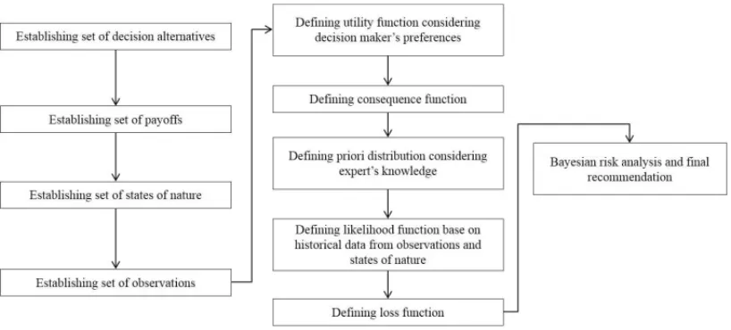
A similar formulation for modelling an investment portfolio decision problem is presented by Ferreira et al. (2009). Their paper presented a decision model built from a set of decision alter-natives for investment, a set of the returns on investment, a set of ambient conditions, a set of macroeconomic and microeconomic factors. How they interacted was brought about by proba-bility mechanisms that lead to effective Bayesian Risk Analysis, the measure used to validate the assumptions of decision analysis to evaluate the decisions on the context studied. Thus, Fig-ure 1 gives a similar representation which shows the process for solving the decision problem approached in this paper, and establishing what is known and what could be done.
The set of decision alternatives establishes the possible investment options for allocating the available resources, which in this paper is represented by raw sugarcane. Therefore, the DM’s objective is to maximize the return while minimizing losses.
Thus, the set of decision alternatives is represented by all combinations of the allocation of the available capital (raw sugarcane) among the assets selected. Therefore, this set is represented by A = {a1,a2, . . . ,an}, whereai is the portion of capital, this being limited tonassets being
available for selection in the decision context (Raiffa & Schlaifer, 1961; Berger, 1985) and the constraint is satisfied that all capital must be allocated to the assets, withA=n
j=1aj =1.
The payoffs are consequences associated with the investment options and are treated as gains and/or losses which are delivered to the DM and they are represented by the return on investment in certain assets invested in the capital market. This set is expressed by B = {b1,b2, . . . ,bn},
Figure 1– Structure of the Decision model.
Given that the return on an asset over a given period corresponds to the ratio between the differ-ence of the value of the asset in the current period and the previous period and its value in the previous period.rt is the return on an asset in periodt, andVt is its value in periodt.
Thus, it is possible to represent the cumulative return of an asset in periodt, given that this is the multiplicand within the range of returns, soRt =ti=1(1+ri). The cumulative returns result in
a setR= {Rt1,Rt2, . . . ,Rt n}. Based on these data, one can evaluate the set of payoffs resulting
in a cumulative rate of return on each asset in a given period multiplied by the percentage of invested capitalC. Therefore, we may say that B is described as (4), which is expressed in monetary values byB =C∗n
i=1ai ∗Rt i.
There are outcomes over which the DM has no control, namely states of nature, which are rep-resented by the setθ = {θ1, θ2, . . . , θn}(Raiffa & Schlaifer, 1961; Berger, 1985). The states of
nature for the problem addressed in this paper are summarized by positive or negative returns obtained in a given period for each investment asset. Thus, the partial state of nature that can be obtained byθt, when Rt is the cumulative return of an asset in a time interval as described
by (1):
θt =
1, ifRt >0 0, ifRt =0
(1)
The set of observations,X = {x1,x2, . . . ,xn}, can be represented by macroeconomic and
mi-croeconomic factors, which in general are available to the DM and can be analysed to establish correlations with the state of nature. In this paper observations are considered to be variations in an economic index, such asKt, thus, an observation is represented by (2):
Xt =
1, ifKt >0
0, ifKt =0
The utility function enables consideration to be given to a DM’s risk behaviour (averse, neutral and prone) and therefore the degree of aversion or propensity or neutrality toward risk that the DM has to define. The utility function considered for this problem is a linear representation which satisfies decision analysis standard conditions (Raiffa & Schlaifer, 1961; Berger, 1985), represented by the variation in investment gains by adopting lower and upper values, given by (3):
U(b)= b−min(b)
max(b)−min(b) (3)
U(b)is the utility of a payoff b, min(b)is the minimum expected return, and max(b)is the maximum expected return.
The consequence function is obtained from a statistical analysis of historical data for the assets selected, as a probability distribution (Ferreira et al., 2009). For instance, if the data fit a normal distribution, this function is given by (4):
P(b|θ ,a)= n
i=1
aiP(b|θ )= n
i=1
ai Normal(b, µθi, σθi) (4)
whereµθi is the estimated average for the value of asseti, andσθi is the standard deviation for
the value of asseti.
The states of nature involved may be explained by a priori knowledge. Thus, it is possible to associate a priori probability distribution over states of nature, which is represented byπ(θ )
(Bernoulli, 1954; Bernardo & Smith, 1994; Ferreira et al., 2009). For the problem formulated in this paper, a priori distribution can be constructed from the relative frequency of cumulative return rates over time on the sugarcane output commodities.
The likelihood function offers probabilistic information of a particular variable observed so as to discover whether a particular state of nature occurred in a time interval. The mathematical representation of this function corresponds to P(x|θ ), which responds to the model using his-torical data from observations and the variables associated with states of nature in a specific context (Raiffa & Schlaifer, 1961; Berger, 1985; Bernardo & Smith, 1994; Ferreira et al., 2009). Thus, the likelihood function can be represented by a vector of dimension equal to the number of observations multiplied by the number of states of nature.
The combination of the a priori distribution and a likelihood function results in the a posteriori distribution. This distribution is used for the calculations of Bayes’s rules to describe the prob-ability of states of nature after a given known variable has been observed (Raiffa & Schlaifer, 1961; Berger, 1985; Bernardo & Smith, 1994; Ferreira et al., 2009):
P(x, θ )=π(θ )P(x|θ ) (5)
P(x)=
θ
P(x, θ )=
θ
π(θ )P(x|θ ) (6)
Therefore, the a posteriori distribution is given by (7):
π(θ|θx)= P(x, θ )
The loss function is recognized as the opportunity cost (i.e., the cost of choosing one alternative over another decision) in a given situation, as given by (8) (Raiffa & Schlaifer, 1961; Berger, 1985; Bernardo & Smith, 1994; Ferreira et al., 2009):
L(θ ,a)= − b
U(b)P(b|θ ,a)db (8)
From this perspective, the risk function is defined as the expected loss of a given situation, which corresponds to the average loss obtained when choosing a specific action, assuming thatθis the true state of nature. Thus, the risk function (Raiffa & Schlaifer, 1961; Berger, 1985; Ferreira et al., 2009) represents the expected value expected of the random variableL(θ ,a):
Ra(θ )=
x
L(θ ,a)P(x|θ )=Eθ[L(θ ,a)] (9)
Therefore, in a Bayesian risk analysis perspective,rais a measure that considers a priori
knowl-edge about the state of nature so as to determine the probability of obtaining a certain payoff that plays a significant part in the decision context – in other words,ra measures the risk of an
action given thatxoccurred (Raiffa & Schlaifer, 1961; Berger, 1985; Bernardo & Smith, 1994; Ferreira et al., 2009), given by (10) and (11). This metric allows decision rules to be established, wherera is the risk of a decision ruleRagiven by the utility ratio in a state of natureθ:
ra = −u(P(b|a)) (10)
ra=
θ
π(θ ) x
P(x|θ )L(θ ,d(x))=
θ
π(θ )Ra(θ ) (11)
Equation (11) shows the value of the Bayes risk of the decision rule. The interpretation of the results obtained by these rules is conducted by checking the lowest risk for a particular context, given the preferences of maximizing gains and minimizing the risks associated with the deci-sion process. In other words, the action chosen will be the one that minimizesra for a given
observation.
3 CASE STUDY
In Brazil, there are many producers of sugarcane who are responsible for processing and trans-forming raw sugarcane into its derived commodities. Therefore, these producers assume the responsibilities of the DM in this capital investment process in the sugarcane industry.
The Brazilian sugarcane industry has three main assets: crystal sugar and anhydrous and hy-drous ethanol. For this proposed application, these assets are sufficient to show the results of the decision model. The set of assets is represented by random variables in the decision model:
a1: crystal sugar,a2: anhydrous ethanol, anda3: hydrous ethanol.
price of crystal sugar and anhydrous and hydrous ethanol, extracted from the CEPEA/ESALQ (2014) in the period from January 2005 to December 2014:
Table 1– Descriptive analysis of prices of selected assets (R$ per unit).
Assets Maximum Average Minimum Crystal Sugar 1.5258 0.9185 0.4646 Anhydrous Ethanol 2.3421 1.0826 0.6608 Hydrous Ethanol 1.4606 0.9505 0.5804
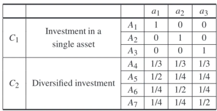
The set of actions is presented in Table 2, and shows possibilities for allocating raw sugarcane into different assets, thus enabling finite combinations to be listed. For simplification purposes, the set of actions is limited to seven elements categorized into two classes. The first class C1
represents the investment in a single sugarcane commodity (A1, A2, and A3) and the second class,C2represents diversified sugarcane commodities (A4,A5,A6, andA7).
Table 2– Set of decision alternatives.
a1 a2 a3
C1
Investment in a A1 1 0 0
single asset A2 0 1 0
A3 0 0 1
C2 Diversified investment
A4 1/3 1/3 1/3
A5 1/2 1/4 1/4
A6 1/4 1/2 1/4
A7 1/4 1/4 1/2
The portion indicated in each asset is equal to the percentage of the amount at a level equivalent to[0,1], where 1 corresponds to 100% of the amount; the same interpretation can be made about the other percentage values.
The consequences are obtained from earnings and/or losses in each percentage of the amount invested in an asset. It is assumed that the payoffs are obtained from the cumulative return of the price of each sugarcane commodity within six months(t =6)in a given period, considering the data collected.
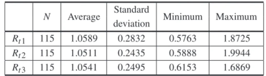
Table 3 represents the descriptive statistics built on the cumulative return on assets, as follows:
Rt1, the cumulative return for crystal sugar; Rt2, the cumulative return for anhydrous ethanol, andRt3, the cumulative return for hydrous ethanol.
Table 3– Descriptive statistics of cumulative return (R$ per 50 kg sack).
N Average Standard Minimum Maximum deviation
Rt1 115 1.0589 0.2832 0.5763 1.8725
Rt2 115 1.0511 0.2435 0.5888 1.9944
Rt3 115 1.0541 0.2495 0.6153 1.6869
The set of states of nature is a discrete set represented by values obtained from the cumulative returns on investments in assets in the sugarcane industry. These values will account for the variation in cumulative returns over the previous period and can be written as a vector of three coordinates, when each one represents the cumulative returns of these assets. Table 4 shows the elements of the sets of states of nature.
Table 4– Frequency of states of nature.
[Rt1,Rt2,Rt3]
Observed Relative frequency percentage (%) θ0 [0,0,0] 31 26.96 θ1 [1,0,0] 17 14.78
θ2 [0,1,0] 3 2.61
θ3 [1,1,0] 4 3.48
θ4 [0,0,1] 4 3.48
θ5 [1,0,1] 3 2.61
θ6 [0,1,1] 16 13.91 θ7 [1,1,1] 37 32.17
The context of the Brazilian economy offers macroeconomic variables that are associated with these outcomes. For this specific context, five variables were selected to build the set of observa-tions:
• x1: The GDP of Brazil is an indicator from which the potential economic activity of a region can be identified.
• x2: The BOVESPA Index is a performance indicator based on the average price that stocks are traded at on the Brazilian stock market, the main purpose of which is to give the ap-proximate range of the configuration about the context of negotiations in the stock market.
• x3: The SELIC Rate is used as a benchmark for monetary policy and indicates the interest rates charged by the Brazilian market.
• x4: The Extended Consumer Price Index (IPCA) aims to show the variation in trade prices to the consumer, defined in economic terms as the price to the end consumer.
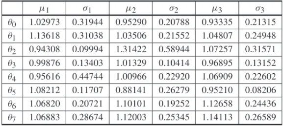
Based on the consequence function, historical data of the cumulative returns are evaluated to verify the adherence to a probability distribution. The data on the price of commodities is as-sumed to be normal which allows P(b|θ ,a)to be written as in (8). Table 5 shows the findings.
Table 5– Average and standard deviation estimated for the cumulative return of each asset.
µ1 σ1 µ2 σ2 µ3 σ3
θ0 1.02973 0.31944 0.95290 0.20788 0.93335 0.21315 θ1 1.13618 0.31038 1.03506 0.21552 1.04807 0.24948 θ2 0.94308 0.09994 1.31422 0.58944 1.07257 0.31571 θ3 0.99876 0.13403 1.01329 0.10414 0.96895 0.13152 θ4 0.95616 0.44744 1.00966 0.22920 1.06909 0.22602 θ5 1.08212 0.11707 0.88141 0.26279 0.95210 0.08206 θ6 1.06820 0.20721 1.10101 0.19252 1.12658 0.24436 θ7 1.06883 0.28674 1.12003 0.25345 1.14113 0.26589
µ1,µ2, andµ3are the average cumulative returns on the sugarcane commodities of crystal sugar, anhydrous ethanol and hydrous ethanol, respectively, considering the relative state of nature. Andσ1,σ2, andσ3are the standard deviations in crystal sugar, anhydrous ethanol and hydrous ethanol, respectively, considering the relative state of nature.
The likelihood function(P(x|θ ))provides the probability of a scenarioXbeing observed, given a specific state of nature. The values estimated can be represented as a relative frequency, and they are presented in Table 6, where blank cells represent the absence of estimates for the values.
Values of X =6,X =18,X =19,X =27,X =29,X =30, andX =31 were excluded for want of occurrence.
By using the utility function, a DM can express his/her preferences and define the extent to which they are willing to run the risks associated with a given situation. For the case under study, the set of payoffs is defined by the limits of the DM’s preferences, given the investment situation in the sugarcane industry. These limits are represented by the vector B = [0.54;1.7], considering the limits of the average cumulative returns among the three assets. Thus, it is as-sumed that the DM expects to receive a payoff between 54% and 170% of the amount invested in a certain asset.
The loss function enables the opportunity cost of an action in a decision context to be calculated. Thus, it is possible to obtain the values for the categories of investments mentioned. From the set of decision alternatives, it is possible for results to be separated into two categories:
• C1: Investment in a single asset;
• C2: Diversified investment among the set of assets.
CategoryC1is allocated alternativesA1,A2, andA3. CategoryC2is allocated alternatives A4,
Table 6– Likelihood function.
X {x1,x2,x3,x4,x5} θ0 θ1 θ2 θ3 θ4 θ5 θ6 θ7
X =0 {0,0,0,0,0} 0.161 0.059 0.250 0.333 0.063 0.108
X =1 {1,0,0,0,0} 0.032 0.250 0.333 0.063 0.027
X =2 {0,1,0,0,0} 0.118 0.250 0.063
X =3 {1,1,0,0,0} 0.333 0.063
X =4 {0,0,1,0,0} 0.097 0.118 0.108
X =5 {1,0,1,0,0} 0.129 0.118 0.250 0.250 0.063 0.135
X =7 {1,1,1,0,0} 0.065 0.059 0.250 0.063
X =8 {0,0,0,1,0} 0.129 0.118 0.250 0.135
X =9 {1,0,0,1,0} 0.065 0.081
X=10 {0,1,0,1,0} 0.065 0.118
X=11 {1,1,0,1,0} 0.059 0.054
X=12 {0,0,1,1,0} 0.125 0.027
X=13 {1,0,1,1,0} 0.065 0.118 0.250 0.333 0.125 0.081
X=14 {0,1,1,1,0} 0.125 0.027
X=15 {1,1,1,1,0} 0.054
X=16 {0,0,0,0,1} 0.027
X=17 {1,0,0,0,1} 0.032 0.333 0.027
X=20 {0,0,1,0,1} 0.032 0.063
X=21 {1,0,1,0,1} 0.027
X=22 {0,1,1,0,1} 0.125
X=23 {1,1,1,0,1} 0.059 0.333
X=24 {0,0,0,1,1} 0.032 0.054
X=25 {1,0,0,1,1} 0.027
X=26 {0,1,0,1,1} 0.065 0.059 0.063
X=28 {0,0,1,1,1} 0.032
Table 7– Loss function.
A1 A2 A3 A4 A5 A6 A7
θ0 –0.59567 –0.75700 –0.79356 –0.71541 –0.68548 –0.72581 –0.73495 θ1 –0.44608 –0.58818 –0.56606 –0.53344 –0.51160 –0.54713 –0.54160 θ2 –0.97370 –0.36388 –0.52945 –0.62234 –0.71018 –0.55773 –0.59912 θ3 –0.74755 –0.71256 –0.82341 –0.76118 –0.75777 –0.74902 –0.77674 θ4 –0.65614 –0.63492 –0.52601 –0.60569 –0.61830 –0.61300 –0.58577 θ5 –0.46789 –0.82266 –0.99192 –0.76083 –0.68759 –0.77629 –0.81860 θ6 –0.53537 –0.44163 –0.42585 –0.46762 –0.48456 –0.46112 –0.45717 θ7 –0.53993 –0.43622 –0.41288 –0.46301 –0.48224 –0.45631 –0.45047
option of investment, considering certain elements of the context. Table 8 presents the results for the categories selected. In this table, the emphasis is placed on alternative decisions with the lowest risk in a given contextual situation of the sugarcane commodities, considering the variables selected for this study.
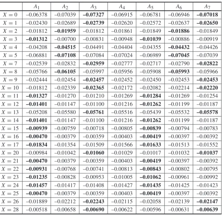
Table 8– Bayesian risk analysis.
A1 A2 A3 A4 A5 A6 A7
X=0 –0.06378 –0.07039 –0.07327 –0.06915 –0.06781 –0.06946 –0.07018
X=1 –0.02430 –0.02689 –0.02739 –0.02620 –0.02572 –0.02637 –0.02650
X=2 –0.01812 –0.01959 –0.01812 –0.01861 –0.01849 –0.01886 –0.01849
X=3 –0.01312 –0.00700 –0.00831 –0.00948 –0.01039 –0.00886 –0.00919
X=4 –0.04208 –0.04515 –0.04491 –0.04404 –0.04355 –0.04432 –0.04426
X=5 –0.06881 –0.07108 –0.07084 –0.07024 –0.06989 –0.07045 –0.07039
X=7 –0.02539 –0.02832 –0.02959 –0.02777 –0.02717 –0.02790 –0.02822
X=8 –0.05766 –0.06105 –0.05997 –0.05956 –0.05908 –0.05993 –0.05966
X=9 –0.02444 –0.02454 –0.02457 –0.02452 –0.02450 –0.02453 –0.02453
X=10 –0.01812 –0.02339 –0.02365 –0.02172 –0.02082 –0.02214 –0.02220
X=11 –0.01327 –0.01270 –0.01210 –0.01269 –0.01284 –0.01269 –0.01254
X=12 –0.01401 –0.01147 –0.01100 –0.01216 –0.01262 –0.01199 –0.01187
X=13 –0.05208 –0.05580 –0.05761 –0.05516 –0.05439 –0.05532 –0.05578
X=14 –0.01401 –0.01147 –0.01100 –0.01216 –0.01262 –0.01199 –0.01187
X=15 –0.00939 –0.00759 –0.00718 –0.00805 –0.00839 –0.00794 –0.00783
X=16 –0.00470 –0.00379 –0.00359 –0.00403 –0.00419 –0.00397 –0.00392
X=17 –0.01834 –0.01354 –0.01509 –0.01566 –0.01633 –0.01513 –0.01552
X=20 –0.00984 –0.01042 –0.01060 –0.01029 –0.01017 –0.01032 –0.01037
X=21 –0.00470 –0.00379 –0.00359 –0.00403 –0.00419 –0.00397 –0.00392
X=22 –0.00931 –0.00768 –0.00741 –0.00813 –0.00843 –0.00802 –0.00795
X=23 –0.01235 –0.00828 –0.00953 –0.01005 –0.01062 –0.00961 –0.00992
X=24 –0.01457 –0.01417 –0.01408 –0.01427 –0.01435 –0.01425 –0.01423
X=25 –0.00470 –0.00379 –0.00359 –0.00403 –0.00419 –0.00397 –0.00392
X=26 –0.01889 –0.02212 –0.02243 –0.02115 –0.02058 –0.02139 –0.02147
X=28 –0.00518 –0.00658 –0.00690 –0.00622 –0.00596 –0.00631 –0.00639
The results shown in Table 8 lead to an indication of the best actions for the investor, considering the scenario observed. The risk calculated for each scenarioXiand for each alternativeAi, shown
in the respective cells. Thus, each scenario can be compared with the others evaluated under each alternative, observing the value of the risk.
For Case 1 (C1), or Category 1, if we assume the set of observations to beX = {x3,x11,x12,x14,
x15,x16,x17,x21,x22,x23,x24,x25}(i.e., the best investment asset), the portfolio that best meets the DM’s expectations is the one for crystal sugar, for which actionA1is recommended. When
X = {x2,x4,x5,x8}, the best investment portfolio is the one for anhydrous ethanol, for which action A2 is recommended. And when X = {x0,x1,x7,x9,x10,x13,x20,x26,x28}, the best portfolio is the one for hydrous ethanol, for which actionA3is recommended.
For Case 2 (C2), or Category 2, if we assume the set of observations is X = {x3,x11,x12,x14,
x15,x16,x17,x21,x22,x23,x24,x25}, the best action to choose for the investment leads to A5, which means that an investment of 50% in sugar, 25% in anhydrous ethanol, and 25% in hydrous ethanol should be made whenX = {x2,x4,x5,x8},A6is recommended, which is equivalent to making an investment of 50% in anhydrous ethanol, 25% in sugar, and 25% in hydrous ethanol and whenX = {x0,x1,x7,x9,x10,x13,x20,x26,x28}, actionA7is suggested, which means mak-ing a 50% investment in hydrous ethanol, 25% in sugar, and 25% in anhydrous ethanol. Note that there is no recommendation that a uniform distribution of investment capital should be made in these assets, represented byA4.
Figure 2 gives the graphical comparison between these two scenarios, or categories.
-0,08 -0,07 -0,06 -0,05 -0,04 -0,03 -0,02 -0,01 0
0 1 2 3 4 5 7 8 9 10 11 12 13 14 15 16 17 20 21 22 23 24 25 26 28
Bay
es Risk
Observations
Case1 Case 2
Figure 2– Comparison of the categories of investment for each state’ observation.
Drawing on Figure 2, a critical analysis can be made as to the extent of the risks calculated for these two categories of investment in the sugarcane sector for the case study. The concentration of lower risk investment options on a single asset is due to the expected value of the cumulative return on assets being used as a reference for the calculations.
derived from the sugarcane industry. However, depending on the DM’s level of risk aversion, investment decisions for the cases presented may change. This argumentation can be formulated by the small difference in relation to the risk presented in Case 1 and Case 2. This difference may encourage the DM to consider various contextual aspects to formulate production planning for the production of sugarcane-derived products that can satisfy the DM’s expectations about the return on investment.
Risk assessment in decision investment is essential to ensure the financial and production loss in the investment process is minimized according to the DM’s expectations. Thus, different tools are used to measure risk and illustrate the scope of action that is the most appropriate for plan-ning production and applying monetary resources.
Thus, the contribution of Bayes risk enables losses to be minimized on taking a priori knowledge about context aspects to describe the uncertainties in the investment actions into consideration. From this perspective, the decision model and its results represent a significant contribution as a flexible tool for production and strategic management in the investment sector, including in agribusiness.
4 FINAL REMARKS
In Brazil, the context of the sugarcane industry has a great influence on the national economy, so this sector has a strategic impact on several areas of the production sector. From this perspective, the approach considered in this paper allows decision strategies for this sector to be identified and formalized, considering the influence of contextual factors. This contribution allows the producer to obtain efficient information about the investment scenario that best responds to expectations, thereby encouraging economic and social development in various contexts.
The influence of the sugarcane sector on the Brazilian economy contributes to the country having the seventh-largest global economy (IBGE, 2014), which highlights the importance of establish-ing plannestablish-ing strategies accordestablish-ing to the risk associated with investment in this sector. Thus, the study of applications involving the sugarcane industry is timely due to trends of global con-sumption and the search for substitutes for oil, especially those that generate energy. Due to the growing influence of this sector in the market and also to environmental concerns, there is a need to control this development to avoid unknowns.
The flexibility of this method is of considerable interest for producers, technicians, and re-searchers, who are seeking to improve the control and performance of asset management ac-tivities. The contributions of this article indicate that part of the production planning process in the sugarcane industry can be interpreted as an investment analysis, where the values of sug-arcane derivatives are considered to be building investment indicators. Thus, analysis sought to integrate production planning decisions and investment analysis considering the economic par-ticularities and contextual factors in the sugarcane industry, which have significant importance for and influence on the Brazilian economy.
preferences. The contribution of Bayes risk to obtain information about the investment context is suitable and leads to friendly results in decision management as this approach indicates how to minimize loss in the investment process in an organization. Thus, knowledge and management of risk associated with the investment process can be used as performance measures, thereby aiding the process of decision-making.
The application of the decision model explains the contribution of risk analysis to organizations. This analysis enables the fundamentals to be drawn up of best decisions when planning invest-ments, and offers a strategic positionvis-`a-visthe contextual uncertainty. From this perspective, the results obtained used for the decision model define it as a tool that is appropriate in the con-text of portfolio investments in the sugarcane industry, which can be adapted to other portfolio investment contexts.
The calculations used in this paper were supported by Matlab, although using a DSS should be the next step so as to give more flexibility and interactivity to elicit DM risk behaviour and add interactivity to the decision process, which can later be extended to other general portfolio problems.
ACKNOWLEDGMENTS
This work was partially supported by CNPq (Brazilian Research Council) and FACEPE (Foun-dation of Science and Technology of Pernambuco State).
REFERENCES
[1] A¨IT-SAHALIAY & BRANDTMW. 2001. Variable Selection for Portfolio Choice.The Journal of Finance,56: 1297–1351.
[2] ALEXANDERGJ & BAPTISTAAM. 2011. Portfolio selection with mental accounts and delegation.
J. of Banking & Finance,35: 2637–2656.
[3] AVRAMOVD & ZHOU G. 2010. Bayesian Portfolio Analysis.Annual Review of Financial Eco-nomics,2: 25–47.
[4] AZEVEDOJM & GALIANAFD. 2009. The sugarcane ethanol power industry in Brazil: obstacles, success and perspectives. In: Electrical Power & Energy Conference (EPEC), Montreal, QC: IEEE.
[5] BERGERJO. 1985. Statistical Decision Theory and Bayesian Analysis. Springer-Verlag, Berlin.
[6] BERNARDOJ & SMITHA. 1994. Bayesian Theory. John Wiley & Sons, New York.
[7] BERNOULLID. 1954. Exposition of a New Theory on the Measurement of Risk.Econometrica,22: 23–36.
[8] BRANDTMW. 1999. Estimating Portfolio and Consumption Choice: A Conditional Euler Equations Approach.The Journal of Finance,54: 1609–1645.
[9] BURASCHIA, PORCHIAP & TROJANIF. 2010. Correlation Risk and Optimal Portfolio Choice.
Journal of Finance,65: 393–420.
[11] CLARKSONGP & MELTZERAH. 1960. Portfolio Selection: A Heuristic Approach.The Journal of Finance,15: 465–480.
[12] COHENKJ & POGUEJA. 1967. An Empirical Evaluation of Alternative Portfolio-Selection Models.
The Journal of Business,40: 166–193.
[13] DELIMAJRMP & FERREIRARJP. 2013. Algoritmo para Selec¸˜ao Discreta de Lotes de Ativos com Base em Busca Tabu.PODes,5: 113–135.
[14] FERREIRARJP, ALMEIDA-FILHOAT & SOUZAFMC. 2009. A Decision Model for Portfolio Se-lection.Pesquisa Operacional,29: 403–417.
[15] GARTNERIR. 2012. Differentiated risk models in portfolio optimization: Comparative analysis of the degree of diversification and performance in the S˜ao Paulo stock exchange (BOVESPA).Pesquisa Operacional,32(2): 271–292.
[16] GARVEYMD, CARNOVALES & YENIYURTS. 2015. An analytical framework for supply network risk propagation: A Bayesian network approach.European Journal of Operational Research,243(2): 618–627.
[17] GUOX, WONGW-K, XUQ & ZHUX. 2015. Production and hedging decisions under regret aver-sion.Economic Modelling,51: 153–158.
[18] IBGE. 2014.<www.ibge.gov.br>. Accessed in October, 2014.
[19] JIANG CH, MAYK & AN YB. 2010. An analysis of portfolio selection with background risk.
Journal of Banking & Finance,34: 3055–3060.
[20] KALATZISAEG, AZZONICR & ACHCARJA. 2006. Uma abordagem bayesiana para decis˜oes de investimentos.Pesquisa Operacional,26(3): 585–604.
[21] KNIGHTFH. 1921. Risk, Uncertainty and Profit. New York: Hart, Scharffner and Marx.
[22] LOVISOLOHJ & LEALRPC. 2013. Black Swans in the Brazilian Stock Market.Pesquisa Opera-cional,33(2): 235–250.
[23] LUO C, SECO L & WUL-L B. 2015. Portfolio optimization in hedge funds by OGARCH and Markov Switching Model.Omega,57: 34–39.
[24] MAGO`ET & MODAVEF. 2011. The optimality of non-additive approaches for portfolio selection.
Expert Systems with Applications,38: 12967–12973.
[25] MANSINIR & SPERANZAMG. 1999. Heuristic algorithms for the portfolio selection problem with minimum transaction lots.European Journal of Operational Research,114: 219–233.
[26] MARKOWITZH. 1952. Portfolio Selection.The Journal of Finance,7: 77–91.
[27] MARKOWITZ H. 2014. Mean-variance approximations to expected utility. European Journal of Operational Research,234(2): 346–355.
[28] OLIVEIRA SC & ANDRADEMG. 2012. Comparison between the complete Bayesian method and empirical Bayesian method for ARCH models using Brazilian financial time series.Pesquisa Opera-cional,32(2): 293–313.
[29] P ´ASTORL & STAMBAUGHRF. 2000. Comparing asset pricing models: an investment perspective.
[30] P ´ASTORL. 2000. Portfolio Selection and Asset Pricing Models.The Journal of Finance,55: 179– 223.
[31] RAIFFAH & SCHLAIFERR. 1961. Applied statistical decision theory. Clinton Press Inc., Boston.
[32] ROBBINS H. 1964. The Empirical Bayes Approach to Statistical Decision Problems. Annals of Mathematical Statistics,35: 1–20.
[33] RUBINSTEINM. 2002. Markowitz’s ’Portfolio Selection’: A fifty-year retrospective.The Journal of Finance,62: 1041–1045.
[34] SPERANZAMG. 1996. A heuristic algorithm for a portfolio optimization model applied to the Milan stock market.Computers and Operations Research,23: 433–441.
[35] TOBINJ. 1958. Liquidity Preference as Behavior Towards Risk.The Rev of Econ Studies,25.