FILTRAGEM COLABORATIVA APRIMORADA:
RAMON PEREIRA. LOPES
FILTRAGEM COLABORATIVA APRIMORADA:
EXPLORANDO SIMILARIDADES.
Tese apresentada ao Programa de Pós--Graduação em Ciência da Computação do Instituto de Ciências Exatas da Universi-dade Federal de Minas Gerais como req-uisito parcial para a obtenção do grau de Doutor em Ciência da Computação.
Orientador: Renato Martins Assunção
Coorientador: Rodrygo Luis Teodoro Santos
Belo Horizonte
RAMON PEREIRA. LOPES
SIMILARITY-ENHANCED COLLABORATIVE
FILTERING.
Thesis presented to the Graduate Program in Computer Science of the Universidade Federal de Minas Gerais in partial fulfill-ment of the requirefulfill-ments for the degree of Doctor in Computer Science.
Advisor: Renato Martins Assunção
Co-Advisor: Rodrygo Luis Teodoro Santos
Belo Horizonte
Lopes, Ramon Pereira.
L864s Similarity-enhanced Collaborative Filtering. / Ramon Pereira. Lopes. — Belo Horizonte, 2017
xxiv, 77 f. : il. ; 29cm
Tese (doutorado) — Universidade Federal de Minas Gerais – Departamento de Ciência da Computação
Orientador: Renato Martins Assunção Coorientador: Rodrygo Luis Teodoro Santos
1. Computação – Teses. 2. Sistemas de
recomendação. 3. Filtragem colaborativa. 4. Teoria dos grafos. 5. Teoria bayesiana de decisão estatística. I. Orientador. II. Coorientador. III. Título.
Acknowledgments
Aos meus orientadores, Profs. Renato Assunção e Rodrygo Santos, na falta de palavras para expressar minha profunda e eterna gratidão, recorro à singeleza de um muito obrigado.
Aos Profs. Euclimar e Ninfa, agradeço pelo financiamento de meus estudos pelos sete primeiros anos de minha vida escolar. Esse ato de generosidade foi o ponto germinal para esta tese de doutorado.
Aos Profs. Alexandre Salles, Flávio Assis e Thiago Noronha, agradeço pelos ensinamentos e orientação nas primeiras etapas dessa longa caminhada acadêmica.
À minha família, Edna, Larissa e Raimundo, agradeço pelo incentivo e apoio incondicional ao longo dessa jornada.
À Patrícia, agradeço por todo açúcar e afeto, além das boas risadas. Aos amigos, agradeço pelo apoio nas horas de dificuldade.
Por fim, agradeço à Coordenação de Aperfeiçoamento de Pessoal de Nível Superior (CAPES) e ao Conselho Nacional de Desenvolvimento Científico e Tec-nológico (CNPq) por ter proporcionado apoio financeiro, e todos aqueles que direta ou indiretamente contribuíram para o desenvolvimento deste trabalho.
“And now that you don’t have to be perfect, you can be good.”
(John Steinbeck)
Resumo
Fatoração de Matrizes (FM) é a técnica de recomendação mais efetiva para filtragem colaborativa. Contudo, o estado-da-arte em FM geralmente requer dados adicionais, os quais podem estar nem sempre disponíveis. Se por um lado modelos de recomen-dação baseados em grafos surgiram recentemente como uma alternativa no contexto de fitragem colaborativa, por outro lado os modelos mais efetivos ignoram tanto o con-junto de notas quanto qualquer noção de confiabilidade nos caminhos que conectam usuários e itens. Neste trabalho, exploramos dados colaborativos com o objetivo de prover recomendações mais precisas nos contextos de FM e de recomendação baseada em grafos. Para esse fim, propomos abordagens baseadas em grafos e três funções de pontuação baseadas no paradigma Bayesiano, e um novo modelo Bayesiano para FM. Nossa abordagem baseada em grafos explora caminhos de comprimento três a partir do usuário alvo no grafo de relacionamentos entre usuários e itens, enquanto as funções de pontuação exploram aspectos distribucionais das notas dadas pelos usuários a fim de extrair informações latentes. Nossa abordagem baseada em FM, por sua vez, explora similaridades tanto entre usuários quanto entre itens, de modo que as similaridades são computadas a partir da matriz de interação entre usuários e itens. Avaliamos o desempenho de nossos métodos em várias coleções de teste disponíveis publicamente e comparamos com outras abordagens da literatura sob um conjunto de métricas. Os resultados mostram que os nossos métodos superam aqueles comparados em vários cenários.
Palavras-chave: Sistemas de Recomendação, Filtragem Colaborativa, Grafos, Fa-toração de Matrizes, Estatística Bayesiana.
Abstract
Matrix factorization (MF) is the most successful recommendation approach in the con-text of Collaborative Filtering (CF). However, existing MF approaches usually demand external data for improved regularization, which limit its applicability as external data are not always available. On the one hand graph-based models have recently emerged as an alternative recommendation approach, on the other hand state-of-the-art graph-based approaches ignore the set of ratings and the reliability of the path connecting users and items. In this dissertation, we exploit collaborative data to improve MF and graph-based recommendation. To be precise, we propose a computationally effi-cient graph-based approach to CF and three scoring functions based on the Bayesian paradigm, and a novel MF approach. Our graph-based approach exploits three-step paths starting from the target user in the user-item bipartite graph and relies on the scoring functions, which exploit distributional aspects of the ratings given by users to extract latent information. Our MF approach, in turn, exploits both user-user and item-item similarities extracted from the raw user-item rating matrix. We experiment with several publicly available datasets against state-of-the-art baselines. The results attest the value of our methods as they provide significant gains in several settings.
Palavras-chave: Recommender Systems, Collaborative filtering, Graph-based recom-mendation, Matrix Factorization, Bayesian statistics.
List of Figures
1.1 Recommendation list for a Netflix user. . . 3
1.2 Memory-based representation for 3 users and 4 items, where a missing entry is represented by a dash. . . 4
1.3 Graph-based representation for the instance illustrated in Figure 1.2. . . . 5
1.4 429 customer reviews and 4 stars average rating. . . 7
1.5 3 customer reviews and 5 stars average rating. . . 7
2.1 Example of a transition matrix P. . . 24
3.1 User-item bipartite graph. . . 32
3.2 MAP breakdown for users with various levels of sparsity. . . 52
3.3 MAP breakdown for users with various levels of sparsity. . . 53
3.4 Zoom into MAP breakdown for users with various levels of sparsity. . . 53
4.1 Graphical model for PMF. . . 56
4.2 Graphical model for SMF. . . 57
4.3 MAP breakdown for users with various levels of sparsity. . . 65
4.4 MAP breakdown for active users on ML 1M. . . 66
List of Tables
3.1 Datasets properties. . . 40 3.2 Best parameter configuration for each dataset. . . 44 3.3 Performance comparison of our method and baselines on BX dataset. . . . 46 3.4 Performance comparison of our method and baselines on CDs dataset. . . . 47 3.5 Performance comparison of our method and baselines on Electronics dataset. 48 3.6 Performance comparison of our method and baselines on Epinions dataset. 49 3.7 Performance comparison of our method and baselines on Kindle dataset. . 50 3.8 Performance comparison of our method and baselines on MovieLens 1M
dataset. . . 51
4.1 Performance comparison of our method and baselines on BX dataset. . . . 60 4.2 Performance comparison of our method and baselines on CDs dataset. . . . 61 4.3 Performance comparison of our method and baselines on Epinions dataset. 62 4.4 Performance comparison of our method and baselines on MovieLens 1M
dataset. . . 63
5.1 Comparison between Categorical Inequality Scoring (CIS) and Weighted Regularized Matrix Factorization (WRMF) for each dataset. . . 68 5.2 Comparison between CIS and Similarity-based Matrix Factorization (SMF)
for each dataset. . . 69
Acronym List
AP Average Precision
BIS Binary Inequality Scoring
BJS Binary Joint Scoring
BORS Binary Odds Ratio Scoring
BPRMF Bayesian Personalized Ranking Matrix Factorization
BX BookCrossing
CF Collaborative Filtering
CIS Categorical Inequality Scoring
MAP Mean Average Precision
MF Matrix Factorization
ML Movie Lens
MP Most Popular
MRR Mean Reciprocal Rank
nDCG Normalized Discounted Cumulative Gain
P Precision
PMF Probabilistic Matrix Factorization
RR Reciprocal Rank
RRW Rating-based Random Walk
RS Recommender Systems
SMF Similarity-based Matrix Factorization
SVD Singular Value Decomposition
WRMF Weighted Regularized Matrix Factorization
Contents
Acknowledgments ix
Resumo xiii
Abstract xv
List of Figures xvii
List of Tables xix
Acronym List xxi
1 Introduction 1
1.1 Preliminaries . . . 1 1.2 Motivation . . . 6 1.2.1 Exploitation of the user-item matrix . . . 7 1.2.2 Markovian Property . . . 7 1.2.3 Space and Time Complexity . . . 8 1.3 Hypothesis and Goals . . . 8 1.4 Contributions . . . 9 1.5 Thesis Organization . . . 11
2 Background and Literature Review 13
2.1 The Recommendation Problem . . . 13 2.2 Content-based Recommendation . . . 15 2.3 Collaborative Filtering Recommendation . . . 17 2.3.1 Memory-based Approaches . . . 18 2.3.2 Model-based Approaches . . . 26
3 Graph-based Recommendation Approaches 31
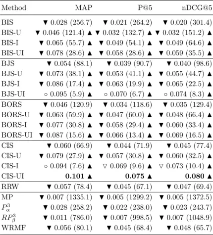
3.1.2 Categorical Rating Model . . . 33 3.2 Algorithms . . . 33 3.2.1 Rating-based Random Walk . . . 33 3.2.2 Scaled Path Scoring . . . 35 3.2.3 Bayesian Scoring Functions . . . 37 3.3 Experimental Setup . . . 40 3.3.1 Datasets . . . 40 3.3.2 Evaluation Methodology . . . 41 3.3.3 Evaluation Criteria . . . 42 3.3.4 Recommendation Baselines and Parameter Tuning . . . 43 3.4 Experimental Results . . . 44 3.4.1 Scaling Strategy and Scoring Functions Choice . . . 45 3.4.2 Recommendation Effectiveness . . . 45 3.4.3 Recommendation Robustness . . . 47 3.5 Discussion . . . 50
4 SMF: Similarity-based Matrix Factorization 55
4.1 SMF Model . . . 55 4.1.1 Probabilistic Matrix Factorization . . . 55 4.1.2 Similarity-based Matrix Factorization . . . 56 4.1.3 Inference . . . 58 4.1.4 Complexity Analysis and Implementation Details . . . 58 4.2 Experimental Setup . . . 58 4.3 Experimental Results . . . 60 4.3.1 Similarity Choice . . . 60 4.3.2 Recommendation Effectiveness . . . 62 4.3.3 Recommendation Robustness . . . 63 4.4 Discussion . . . 64
5 Conclusion and Future Work 67
5.1 Concluding Remarks . . . 67 5.2 Future Directions . . . 69
Bibliography 71
Chapter 1
Introduction
In this chapter, we provide a brief introduction to the problem addressed in this dis-sertation. First, we motivate recommender systems and contextualize some state-of-the-art approaches. Next, we discuss some motivations for this dissertation. Finally, we state our hypothesis and summarize our contributions.
1.1
Preliminaries
The emergence of e-commerce platforms has drastically changed the way we shop. First, companies provide customers with a myriad of products and delivery services by means of 24-7 e-commerce sites. Second, shoppers are able to browse a great range of products, search for more specific goods, compare prices and features more easily, and leave reviews on products just by means of a device connected to the Internet wherever they are and whenever they want. On the one hand this scenario encourages people to purchase more products, on the other hand the convenience and availability of products increase the amount of information shoppers must process before they make up their minds. For instance, the Amazon’s Web site1 provides more than 1.8 million books in
the “Business & Money” section. As a result, users usually struggle to find the most appropriate items from the immense variety of items available at these e-commerce Web sites [Ricci et al., 2011].
Das et al. [2007] point out users usually do not even know what they want so that they rely on the Web site to present them something that fulfills their needs. For instance, a user ends up looking around for movies that might interest her instead of browsing for a particular movie she wants to watch. Furthermore, Ricci et al. [2011]
1
www.amazon.com
advocate the great amount of products in e-commerce services overwhelms users, which turns out to lead them to make poor decisions and decrease their well-being. In this context, the use of Recommender Systems (RS) has arisen as an effective solution not only to the information overload problem but also to the improvement of merchant revenue [Jannach et al., 2010; Schafer et al., 1999]. Indeed, these systems provide suggestions for users with the aim at helping in various decision-making processes, such as what items to buy, what music to listen, or what news to read [Ricci et al., 2011].
Schafer et al. [1999] report on several industrial applications of RS technology in e-commerce in the end of 1990’s. In reality, RS help e-commerce increase profits in three ways [Schafer et al., 2001]: i) converting browsers into buyers, ii) suggesting additional products for the customer to purchase based on those products already in the shopping cart, and iii) improving customers’ loyalty in that customers tend to return to the sites that match their needs. Thus, RS play a fundamental role in marketing activities of e-commerce and have become largely utilized in multiple business niches. In fact, the use of RS has exploded over the last decade, where major companies made use of RS within their services [Jannach et al., 2016]. Currently, the use of RS is so pervasive that encompasses plenty of applications, including [Ricci et al., 2011]: i) entertainment: recommendations of movies, music and friends in social networks, ii) content: person-alized news, articles and documents, iii) e-commerce: recommendations for consumers of products in online shopping websites, and iv) services: recommendations of travel services and houses to rent.
Schafer et al. [2001] define RS as specialized data mining systems designed to take advantage of the real-time personalization opportunities of interactive e-commerce. Ricci et al. [2011], in turn, define RS as software tools and techniques providing sug-gestions for items to be of use to a user. Independently of the definition, the main objective of RS is to guide users in a personalized way to interesting products to max-imize users’ satisfaction. For instance, Netflix reports 75% of what their consumers watch come from some sort of recommendation algorithms.2 To this end, these
sys-tems learn from customers, compute recommendations using proper techniques and finally present the recommended products that the shopper will probably find most valuable among those available [Wei et al., 2007]. In fact, the products are usually recommended based on four types of user data [Ricci et al., 2011]: i) data about users and available items, ii) rating or reviews (explicit feedback), iii) behavior (implicit feedback), and iv) transaction.
2
1.1. Preliminaries 3
The forms of recommendation usually include suggesting products to the con-sumer, providing personalized product information, summarizing community opinion, and providing community critiques [Schafer et al., 2001]. Figure 1.1 shows a recom-mendation list for a Netflix user based on the fact the user provided a feedback to the system, namely, the user has watched “Paris, Texas”. Thus, RS are able not only to recommend movies according to the user’s tastes but also to provide explainable recommendations.
Figure 1.1: Recommendation list for a Netflix user.
RS allow personalization for each customer, where users are presented to items according to their tastes. To this end, the recommender acquires and analyzes users’ data, builds a model of consumer behavior, and makes use of algorithms to produce recommendations. In this process, computing recommendations via proper techniques plays a significant role in the quality of the recommendation result [Wei et al., 2007]. Thus, many different approaches have been applied to the problem of making recom-mendations that fit the users’ tastes [Schafer et al., 2001]. For instance, the earliest RS [Resnick et al., 1994; Shardanand and Maes, 1995] make use of nearest-neighbors, where recommendations for a target user are based on similar customers with respect to their preference histories. While the earliest RS dates back to 1990’s, RS have become subject of intense research due to the Netflix Prize3, which began in 2006.
The Netflix Prize was a competition held by Netflix where 51,051 contestants on 41,305 teams from 186 different countries competed for the grand prize of U$1,000,000. Netlifx relied on its own recommendation system Cinematch to predict whether a user will enjoy a movie based on her history and make personalized movie recommendations. In the contest, competitors had to propose algorithms to beat Cinematch by making better predictions, where the winner’s method had to show prediction accuracy at least 10% better than Cinematch. To this end, participants had access to training and qualifying test sets. The training data consisted of more than 100 million ratings from over 480 thousand randomly-chosen, anonymous customers on nearly 18 thousand movie titles. The qualifying data, in turn, contained over 2.8 million customer/movie id
3
pairs with rating dates but with the ratings withheld. After almost three years, Netflix announced the winner with a 10.09% improvement over Cinematch. As a result, much progress has been made in RS, particularly in Collaborative Filtering (CF) [Jannach et al., 2016].
RS fundamentally take one of two approaches, namely, Content-based Filtering or CF, or show a combination of both. Content-based Filtering, which has its roots in information retrieval and information filtering [Adomavicius and Tuzhilin, 2005; Wei et al., 2007], leverages features of items to find similar content. In fact, this sort of systems recommends items similar to those a given user has liked in the past by matching up the attributes of a user profile, in which preferences and interests are stored, with the attributes of candidate items [Lops et al., 2011]. In turn, CF, which is one of the earliest recommendation technologies [Resnick et al., 1994], makes use of the feedbacks other users have provided to recommend items the target user potentially likes best.
In memory-based CF approaches, n users are usually represented as vectors em-bedded in anm-dimensional vector space where each dimension corresponds to an item. Thus, data are represented as an n ×m user-item matrix where rows correspond to users, columns to items and each entry usually represents a rating. As an alternative, items can be represented as vectors embedded in a n-dimensional vector space where each dimension corresponds to a user. Figure 1.2 illustrates the matrix representation for 3 users and 4 items. In reality, most users rate only a small subset of the items and the number of items is much larger than the number of users [Koren et al., 2009].
i1 i2 i3 i4
u1 4 1 − −
u2 4 3 5 −
u3 − 3 − 1
Figure 1.2: Memory-based representation for 3 users and 4 items, where a miss-ing entry is represented by a dash.
1.1. Preliminaries 5
also be based on graph statistics such as commute or hitting time between nodes. For instance, users that possess the same taste will be connected by a large number of short paths [Fouss et al., 2005]. In contrast, classical measures of similarity between users in the context of CF exploit user behavior. To the best of our knowledge, Horting [Ag-garwal et al., 1999] is the first graph-based approach for CF. In particular, nodes are consumers, weighted edges indicate the similarity between two consumers, and recom-mendations are produced by walking the graph to nearby nodes and then combining the opinions of the nearby consumers. Thus, Horting is able to explore transitive relationships that nearest neighbor algorithms do not consider [Sarwar et al., 2001].
u1
u2
u3
i1
i2
i3
i4
Figure 1.3: Graph-based representation for the instance illustrated in Figure 1.2.
In a seminal paper, Page et al. [1999] propose to treat an entity graph as a Markov chain whose long-term stationary distribution can be used as a global scoring. In the literature, there exist several works [Baluja et al., 2008; Christoffel et al., 2015; Cooper et al., 2014; Fouss et al., 2007, 2005; Gori and Pucci, 2007; Jamali and Ester, 2009; Lee et al., 2012; Singh et al., 2007; Xiang et al., 2010; Yildirim and Krishnamoorthy, 2008] that make use of random walks in the context of CF. To this end, transition probabilities are usually defined so that they exploit the user-item graph structure. For instance, the transition probability between two items is proportional to the number of users that rated both items [Gori and Pucci, 2007]. The authors in [Christoffel et al., 2015; Cooper et al., 2014] take a step further and show that it is possible to improve recommendation accuracy by obtaining the distribution within three or five steps instead of incurring the computational burden of obtaining the long-term stationary distribution as in [Fouss et al., 2007, 2005; Gori and Pucci, 2007; Singh et al., 2007].
our approach in several datasets against state-of-the-art approaches, where empirical results attest the effectiveness of our algorithms.
Model-based CF approaches rely on the user-item matrix representation to pro-duce recommendations. In fact, these models exploit collaborative data to learn a pre-dictive model that represents latent characteristics of the users and items in the system with factors in a latent space of reduced dimensionality. In this context, MF [Ko-ren et al., 2009] is the most prominent approach, which regularizes the latent factors through l2-norm. On the other hand, several works [Adams et al., 2010; Agarwal and
Chen, 2009; Porteous et al., 2010; Shan and Banerjee, 2010; Shi et al., 2013; Singh and Gordon, 2008; Yao et al., 2014] extend MF by further regularizing user and/or item factors when side information is available for improving recommendation accuracy. For instance, user side information may comprise age, gender and location, while item side information may include item metadata such as genre, title and reviews. Thus, these works can be regarded as hybrid methods in that they jointly use a collabora-tive filtering technique along with user and/or item profiles to make recommendations. Nonetheless, side information may not be available, limiting the applicability of these works.
Liang et al. [2016] extend MF by jointly factorizing both the user-item interaction matrix and item-item similarity matrix. Different from previous MF extensions, their approach, CoFactor, directly computes item-item similarities from the raw user-item interaction matrix, which makes CoFactor applicable to a wider range of scenarios, including those where no further data are available. On the other hand, CoFactor is designed for implicit feedback domains and only exploits item-item interactions, which makes room for further advances to improve recommendation accuracy. To this end, we here extend MF by further exploiting the user-item rating matrix in that we extract both user-user and item-item matrices to jointly factorize these matrices and the user-item rating matrix. Empirical results attest the effectiveness of embedding both user-user and item-item similarities into MF, where our approach provides more accurate recommendations compared to the variant that only embeds either user-user or item-item similarity matrix.
1.2
Motivation
1.2. Motivation 7
1.2.1
Exploitation of the user-item matrix
Figures 1.4 and 1.5 show two similar products available in Amazon. One can note the product presented in Figure 1.4 has an average rating smaller than that displayed in Figure 1.5. However, the former has 143 times more customer reviews than the latter. Thus, we can ask: which product is more likely to maximize user’s satisfaction?
Figure 1.4: 429 customer reviews and 4 stars average rating.
Figure 1.5: 3 customer reviews and 5 stars average rating.
The state-of-the-art graph-based methods [Christoffel et al., 2015; Cooper et al., 2014] do not exploit any information from the set of items’ ratings. In fact, these methods solely make use of the set of user-item pairs to define the structure of the user-item bipartite graph. Thus, they take into account neither latent information present on the set of ratings nor similarities between users and/or between items to make recommendations. Recalling the scenario presented in Figures 1.4 and 1.5, these state-of-the-art methods treat both items the same under the light of the items’ rating. Therefore, we claim graph-based approaches should exploit the user-item matrix to improve recommendation accuracy.
In the context of MF, CoFactor [Liang et al., 2016] jointly factorizes the user-item interaction matrix and user-item-user-item similarity matrix for implicit feedback settings. However, the authors do not take user-user similarities into consideration. Thus, there is room for further exploitation of the item interaction matrix by extracting user-user similarities and then embedding both user-user-user-user and item-item similarity matrices into MF to improve recommendation accuracy.
1.2.2
Markovian Property
items not consumed by this user. In fact, any odd-length path in the user-item bipartite graph starting from a user ends up in an item.
From Figure 1.3, one can see the path hu1, i1, u2, i3i does end in an item. In
this context, item i3 is a candidate item for recommendation as it is not consumed
by the target user u1, while item i1 is in both users’ history. Thus, we can ask how
item i3 compares to the consumed item i1. Since users usually resort to acquitances
for recommendations and the candidate itemi3 is in u2’s history, we can also ask how
similar usersu1 and u2 are with respect to their tastes.
The methods presented in [Christoffel et al., 2015; Cooper et al., 2014] do not take into account any of these aspects. In fact, these methods show the Markov prop-erty [Norris, 1998], where the probability of moving to the next state depends only on the current state. For instance, the probability of a random walker starting from u1
reachingi3 does not depend on the previous states u1 andi1 but only on u2. Thus, we
claim graph-based approaches should benefit from the consideration of previous states for recommending.
1.2.3
Space and Time Complexity
Due to the size of the transition matrix, the methods presented in [Christoffel et al., 2015; Cooper et al., 2014; Fouss et al., 2007, 2005; Gori and Pucci, 2007; Singh et al., 2007; Yildirim and Krishnamoorthy, 2008] suffer from memory limitation as the dataset size increases. In addition, these methods are computationally intensive as they require matrix multiplications or matrix inversions. To overcome these issues, Christoffel et al. [2015] and Cooper et al. [2014] propose to approximate the final distribution by a sam-pling process. The proposed methods are applicable to medium or large size datasets, but recommendation accuracy depends on the total number of random walks adopted in the sampling process. Therefore, we claim there is a lack of computationally efficient methods in the context of graph-based approaches that do not degrade recommendation accuracy.
1.3
Hypothesis and Goals
1.4. Contributions 9
• graph-based recommendation can benefit from the exploitation of both distribu-tional aspects of the item ratings and similarities between users and/or between items,
• MF should take into account both user-user and item-item similarities to produce more accurate recommendations.
The main goal of this dissertation is to propose and evaluate CF methods that exploit the information contained in the items’ ratings and the similarities between different entities present in the matrix to improve recommendation accuracy. Further-more, the proposed methods should be applicable to larger datasets. To accomplish this goal and test our hypotheses, the specific goals are to:
1. Propose Bayesian scoring functions and path scoring mechanisms to improve graph-based recommendation.
2. Exploit information from states in a path in the user-item graph to improve recommendation accuracy. For instance, given the path hu1, i1, u2, i3i, how does
user u2 (candidate item i2) compare with the target user u1 (item in the user
history i1)?
3. Devise a more computationally efficient strategy to exploit short-length paths in the bipartite user-item graph than the state-of-the-art graph-based methods.
4. Propose a MF model and a computationally efficient inference algorithm that embed both user-user and item-item similarities.
1.4
Contributions
walk CF approach that exploits the set of items’ ratings for item sampling. We carried out experiments on several publicly available datasets and provide a comprehensive empirical evaluation. The results show our better method clearly outperforms the approaches presented in [Christoffel et al., 2015; Cooper et al., 2014] in all metrics and datasets used for comparison. It is common knowledge in the CF literature that MF approaches are the state-of-the-art methods. Thus, we compare our method against a state-of-the-art MF approach and show our method provide better results in all but one dataset. To the best of our knowledge, our methods are the first three-step graph-based approach to exploit distributional aspects of the ratings and take similarities into account to boost recommendation accuracy. This set of contributions is presented in Chapter 3. In fact, preliminary results were published in [Lopes et al., 2016] and we have been working on a paper to be submitted to a top-tier journal where we present our improved models, algorithms and results.
We propose SMF, a MF model that jointly decomposes the user-item rating matrix and both user-user and item-item similarity matrices. In fact, our model makes use of shared latent factors to decompose such matrices, so that similarities play a fundamental role in regularizing the latent factors. Different from most works found in the literature, our approach makes no use of additional data, such as user demographics or item metadata. Our empirical results demonstrate the effectiveness of SMF, with significant improvements over state-of-the-art MF approaches across several publicly available datasets. Moreover, we empirically show SMF improvements are due to the joint factorization of both user-user and item-item similarity matrices. Finally, we also provide a breakdown analysis to better characterize the circumstances where SMF provides substantial improvements. To the best of our knowledge, SMF is the first MF approach to joint factorize both user-item rating matrix and both user-user and item-item similarities matrices. These contributions are discussed in Chapter 4 and were submitted to the 11th ACM Conference on Recommender Systems (RecSys 2017).
1.5. Thesis Organization 11
1.5
Thesis Organization
Chapter 2
Background and Literature Review
In this chapter, we provide background in RS and detail related work. First, we introduce end pose the recommendation problem. After that, we briefly review content-based recommendation. Finally, we discuss CF methods, specially graph-content-based and MF approaches.
2.1
The Recommendation Problem
RS may serve two different purposes. On the one hand, they can be used to stimulate users into doing something such as buying a specific book or watching a specific movie, which turns out to improve merchant revenue. On the other hand, RS can also be seen as tools for dealing with information overload, as these systems aim to select the most interesting items from a larger set [Jannach et al., 2010]. In general, commercial RS present users to the best recommendations in that the set of recommended items might meet user preferences.
RS may generate personalized or personalized recommendations. In non-personalized recommendations, a fixed list of items is presented to any user regardless of his preferences. For instance, items with the highest average rating or the most sold items are recommended. In personalized recommendations, a set of candidate items is suitably chosen depending on the target user’s taste; users with different prefer-ences potentially receive different recommendation lists. As a matter of fact, empirical tests show customers tend to choose more often items suggested based on personalized methods compared to those recommended based on non-personalized approaches [Jan-nach et al., 2016]. In both settings, recommendations are made on the basis of users’ feedback. Thus, RS fundamentally have to implement ways to acquire feedback; these systems may differ in the way they accomplish such task.
Users’ feedback may be acquired by implicitly monitoring user behavior or ex-plicitly asking users about their preferences [Jannach et al., 2010]. In implicit feedback contexts, the feedback is inferred in an implicit way through customer actions such as buying or browsing an item; this sort of feedback is often easier to obtain because users are more likely to interact with items than to explicitly rate them. In explicit feedback contexts, in turn, users explicitly select a rating from a specified evaluation system, which in turn tries to quantify the user satisfaction regarding the item consumed.
The evaluation system may vary with the system; Aggarwal [2016] enumerates several sorts of evaluation systems where the most relevant are: (a) interval-based, where a discrete set of ordered numbers, for example, the Netflix’s 5-star rating system, (b) binary, where user may express only a like or dislike, for example, users express only thumbs-up or thumbs-down in the YouTube’s rating system, and (c) unary, where there is only a mechanism for a user to specify a liking for a item, for example, Facebook only provided in the past a like button to express liking for a post.
The Netflix challenge has profoundly changed the research in RS [Jannach et al., 2016]. First, great advance has been made with respect to the application of machine learning approaches for RS, where various forms of MF and ensemble methods proven to be successful. Second, the challenge led to a formulation of the recommendation problem as one of matrix completion. In this formulation, given an incomplete (usu-ally sparse) user-item interaction matrix for training, the matrix completion problem amounts to predict (or fill in) the unobserved entries [Aggarwal, 2016]. Thus, we can recommend items with the highest predicted ratings to the target user.
2.2. Content-based Recommendation 15
items are usually ranked in a non-increasing order with respect to the predicted scores. Finally, the top-N items in this ranked list are presented to the user, which is based on the fact customers tend to look at and select items at the beginning of a list [Jannach et al., 2010]. This formulation is usually referred to as the top-N recommendation problem.
The personalized recommendation problem can be formally posed as follows [Ado-mavicius and Tuzhilin, 2005]. Let U be the set of users and let I be the set of items that can be recommended. We define κ: U ×I → R a utility function that measures
the utility of an item i∈I to the user u∈U. The recommendation problem amounts to solve the following optimization problem for a target user u∈U:
i⋆u = arg max i∈I
κ(u, i)
where we must find the item i⋆
u that maximizes the the user’s utility. Alternatively, we
can recommend the N best items to a user or a set of users to an item.
The key issue in RS lies in the utility function κ is only known for a subset of
U ×I. As a result, we must resort to techniques for extrapolating the utility function to the whole set. For instance, in the context of matrix completion, the utility of an item is usually represented by a rating, which indicates how much a user liked the item, and the utility function is only defined for those items in the user’s history.
In this context, personalized RS should be able to predict the utility for unknown user-item interactions and make personalized recommendations based on these predic-tions. To this end, several methods from machine learning, approximation theory, and various heuristics have been applied [Adomavicius and Tuzhilin, 2005]. In the rest of this chapter, we discuss two canonical approaches for personalized RS, where we review the most relevant methods and algorithms in the literature for each approach, and refer readers to up-to-date references.
2.2
Content-based Recommendation
Content-based systems are largely used in scenarios where a significant amount of attribute information is available at hand; these attributes, in turn, are usually keywords, which are extracted from the product description [Aggarwal, 2016]. In fact, these systems try to match users to items based on the attributes of the items the user liked. Content-based systems depend on two sources of data [Jannach et al., 2010]: (a) description of items in terms of content attributes, and (b) user profile that describes her interests in terms of preferred item characteristics. Usually, this sort of systems employs feature extraction techniques to convert information from various sources into a suitable vector space representation. In addition, these systems construct a specific model for each user on the basis of her history of either buying or rating items. In content-based recommendation, the utility κ(u, i) of a candidate item i for a target user u is estimated based on the utilities assigned to items in the u’s history that are similar to i. In other words, the system learns to recommend items that are similar to those items the user liked in the past. Let Content(i) be an item profile and letContentP rof ile(u)be a user profile. Since content-based systems are designed mostly to recommend text-based items [Adomavicius and Tuzhilin, 2005], profiles are usually defined as vector of weights. In fact, each weight denotes the importance of the corresponding keyword and is usually determined by the term frequency/inverse document frequency (TF-IDF) [Baeza-Yates and Ribeiro-Neto, 1999]. User profiles are obtained by analyzing the content of the items in the user history. Thus, the utility function is usually defined as follows [Adomavicius and Tuzhilin, 2005]:
κ(u, i) =ContentP rof ile(u)⊗Content(i)
where ⊗ is a heuristic scoring function, such as the cosine similarity measure [Baeza-Yates and Ribeiro-Neto, 1999].
Content-based systems have known drawbacks that limit their applicability [Jan-nach et al., 2010; Lops et al., 2011]. First, these systems are limited by the features extracted from the items to be recommended as content must be in a form that can be parsed automatically. In fact, some domains have issues with automatic feature extraction, such as graphical images, audio streams and video streams. Second, these systems show a overspecialization in that recommendations for a target user are limited to items that are similar to those already rated, that is, these systems are not able to recommend items that are different from anything the user has seen before. Since we focus on CF recommendation in this dissertation, we refer the reader to [Aggarwal, 2016] as an up-to-date reference on the subject.
2.3. Collaborative Filtering Recommendation 17
recommendation overcomes some inherent limitations of content-based recommenda-tion [Desrosiers and Karypis, 2011]: i) items whose content is not available or difficult to obtain can be recommended based on the feedbacks provided by other users, ii) rec-ommendation relies on the quality of items instead of relying on the content, which might not be a proper indicator of quality, and iii) items with very different content can be recommended as similar users might have interests for different items compared to the target user.
2.3
Collaborative Filtering Recommendation
In reality, users often resort to like-minded acquaintances for recommendations [Sinha and Swearingen, 2001]. For instance, to recommend a movie for a target user, we should find other users that have similar tastes with the target user, and recommend those movies most liked by these users. Thus, the recommendation task consists of determining a set of users similar to the target users and then selecting items liked by these users that fit the target user’s tastes. In fact, this is the basic idea of CF recommenders.
The intuition behind CF recommendation is that if users shared the same interests in the past, they may also share similar tastes in the future. Thus, recommendations are based on the user behavior, which can be regarded as item purchases, rentals, clicks or ratings. The term CF is named as such because these systems must filter the most relevant items from a large candidate set, and users implicitly collaborate with one another [Jannach et al., 2010]. For example, suppose user u and v have purchase histories that strongly overlap and u has recently bought an item that v has not yet seen, so it is sensible to present this item to v.
CF recommendation amounts to identify users whose preferences are similar to those of the target user and then recommend items they have liked. In fact, these systems try to predict the utility of items for a target user based on the items previously rated by other users. To be precise, the utilityκ(u, i)of itemifor targetuis estimated based on the utilities κ(u2, i) assigned to item i by other users u2 ∈ U \ {u1} similar
to u [Adomavicius and Tuzhilin, 2005]. Jannach et al. [2010] present several questions that arise in the context of CF recommendation, where the two most relevant are: (a) how to find users (items) similar to the target user (candidate item)? and (b) how to measure similarity between users (items)?
ratings directly in the prediction, and (b) model-based factor algorithms, which learn a predictive model to produce recommendations. These two approaches are discussed next.
2.3.1
Memory-based Approaches
Memory-based (or neighborhood-based) approaches exploit the fact that similar users display close patterns of rating behavior and similar items are prone to receive con-forming ratings [Aggarwal, 2016]. These methods are essentially heuristics where the utility of a candidate item i for target user u is based on an aggregate of the feed-backs provided by the users most similar to useru that have consumed the candidate item [Adomavicius and Tuzhilin, 2005]:
κ(u, i) = aggr
v∈η(u,i)
rvi
wherervirepresents the feedback for userv on itemi, andη(u, i)defines a neighborhood
that contains the users most similar to useru that have rated item i. The underlying assumptions of these approaches are twofold [Jannach et al., 2010]: i) if users had similar consumption behavior in the past they will have similar tastes in the future, and ii) user preferences remain stable and consistent over time. As a matter of fact, an alternative formulation can be obtained by aggregating the feedbacks given to the items most similar to ithat have been consumed by the target user u.
In the literature, there exists two classes of these approaches: (a) User-based: the predicted rating for a candidate item is computed as the weighted average of the ratings provided by thek users most similar to the target user, where each weight is a measure of similarity between the target and the similar user [Resnick et al., 1994], and (b)Item-based: the predicted rating for a candidate item is computed as the weighted average of the ratings provided by the target user for the k items most similar to the candidate item, where each weight is a measure of similarity between the candidate and the similar item [Sarwar et al., 2001]; it was the earliest algorithm of choice by Amazon [Linden et al., 2003]. In conclusion, Sarwar et al. [2001] present empirical evidence that item-based approaches provide better recommendation accuracy than user-based counterparts.
The choice of an aggregation function is a fundamental issue to the recommen-dation accuracy in memory-based approaches. The simplest aggregation function does not take into account the similarity between peers and is defined as the average among the feedbacks: κ(u, i) = |U1
i|
P
2.3. Collaborative Filtering Recommendation 19
consumed item i. In contrast, the most common aggregate function is the weighted sum, which is usually defined as:
κ(u, i) =C X v∈η(u,i)
sim(u, v)×rvi
where C is a normalizing constant. This function weights the feedback provided by a user v similar to user u by a similarity measure between these two users (sim(u, v)), where the more similar these users are the more weight the feedback rvi will carry in the utility function.
In memory-based approaches, we must determine either similar users or similar items. Therefore, a measure of similarity is at the core of these approaches and directly impacts recommendation accuracy. The two most relevant similarity measures in the context of memory-based approaches are discussed next.
The Pearson correlation coefficient between two users u and v is defined by
P earson(u, v) =
P
k∈Iu∩Iv(ruk−µu).(rvk−µv)
qP
k∈Iu∩Iv(ruk−µu)
2.qP
k∈Iu∩Iv(rvk−µv)
2
(2.1)
where Iu denotes the set of items that u rated and µu denotes the average of ratings given by u. In fact, the Pearson correlation takes into account the fact that different users may use the rating scale differently as it uses deviations from the average rating of the corresponding user. The Pearson correlation between two items is accordingly defined.
The cosine similarity measure between two usersu and v is defined by
Cosine(u, v) =
P
k∈Iu∩Ivruk.rvk
qP
k∈Iur
2
uk.
qP
k∈Ivr
2
vk
(2.2)
The cosine similarity measure between two items is accordingly defined. As with the Pearson correlation, ratings can be mean-centered before computing the similarity measure, which gives rise to the so-called adjusted cosine similarity measure. Finally, the Jaccard similarity measure between two users u and v is defined as follows:
Jaccard(u, v) = |Iu∩Iv| |Iu∪Iv|
(2.3)
ratings into account to compute similarities.
Aggarwal [2016] advocates that the adjusted cosine similarity measure gener-ally provides superior results when compared to the Pearson correlation coefficient in the context of item-based approaches. However, the Pearson correlation coefficient is preferable to the cosine similarity measure because the former accounts for the fact that different users exhibit different levels of bias in rating. In the context of user-based approaches, the Pearson coefficient outperforms other measures [Jannach et al., 2010]. In reality, these approaches suffer from computational limitations. As a matter of fact, it is computationally expensive to compute similarities between pairs of users as the dataset size increases since this task retards the recommendation in real-time. To bypass this issue, the most common strategy is to calculate the similarities between all pairs of users or items in advance and recalculate them periodically [Adomavicius and Tuzhilin, 2005]. Thus, the utilities can be efficiently calculated on demand using precomputed similarities. Finally, Aggarwal [2016] advocates the use of similarity values as combination weights is heuristic and arbitrary.
The neighborhood selection plays an important a crucial role in this process. A naive approach amounts to include all users that have consumed itemiin the neighbor-hoodη(u, i)for a target user u. Jannach et al. [2010] advocates this strategy increases the required calculation time and has an effect on the accuracy of the recommendation as the feedbacks of other users who are not really similar to u would be taken into
account. The most effective approaches for reducing the size of the neighborhood are to define a minimum threshold of the similarity or to limit the size to a fixed a number
k and include the k nearest users to the target user in the neighborhood. However, Herlocker et al. [1999] show a trade-off in selecting the ideal threshold in that: i) if the threshold is too high, the neighborhood size will be very small (predictions can be made for very few items), and ii) if the threshold is too low, the neighborhood size are no significantly reduced.
Memory-based approaches are able to capture local associations in the data as they exploit a neighborhood of the target user (candidate item) through similarity measures [Desrosiers and Karypis, 2011]. As a result, these approaches can recommend an item very different from the usual users’ taste or an item not known by the target user if some of his closest neighbors have consumed this item. The main advantages of these approaches are [Desrosiers and Karypis, 2011]: i) simplicity: these methods are simple to implement, ii) justifiability: they provide explainable recommendations since the neighbors might be presented as a justification, and iii) stability: they are little affected by the addition of users, items and feedbacks.
pre-2.3. Collaborative Filtering Recommendation 21
computation of (item-item) similarities, which makes it suitable for large-scale deploy-ments [Linden et al., 2003]. Furthermore, Item-based methods often provide more relevant recommendations because the user’s rating set is used to perform the recom-mendation [Aggarwal, 2016]. For further information on memory-based approaches, we refer the reader to [Aggarwal, 2016; Desrosiers and Karypis, 2011].
2.3.1.1 Graph-based Approaches
In the context of RS, graphs provide a structural representation of the relationships among users, items or both. Graph-based approaches try to overcome the major prob-lem in the computation of similarity in canonical neighborhood-based methods as the former defines similarity with the use of either structural transitivity or ranking tech-niques. In other words, these approaches allow nodes that are not directly connected to influence each other by propagating information along the edges of the graph [Desrosiers and Karypis, 2011], where: i) the greater the weight of an edge, the more information is allowed to pass through it, and ii) the influence of a node on another should be smaller if the two nodes are further away in the graph. Thus, these approaches are more effective for sparse ratings matrices since they exploit structural transitivity of edges for the recommendation process [Aggarwal, 2016].
Graph-based approaches rely on graph models to define neighborhoods and make use of structural transitivity or ranking techniques to produce recommendations [Ag-garwal, 2016]. In fact, the graphs can be constructed on the users, on the items, or on both, where edges encode the similarity or interaction between nodes. The user-item graph is usually defined as an undirected and bipartite graph G = (U ∪I, E), where there exists an edge (u, i) ∈ E if and only if user u has rated item i. For instance, Figure 1.3 displays the user-item bipartite graph for the rating matrix presented in Figure 1.2. In turn, the user (item) graph is defined by an even number of hops in the user-item graph between users (items). Aggarwal [2016] advocates these two sort of graphs are preferred over the user-item graph since they might take into account the number and similarity of common nodes while creating the edges.
achieved with the use of path-based or random walk-based strategies.
In the path-based strategy, the similarity between two nodes is evaluated as a function of the number and the length of paths connecting the two nodes [Desrosiers and Karypis, 2011]. In a seminal paper, Aggarwal et al. [1999] propose a path-based method for CF, where data are modeled as a directed user graph and edges’ weight is determined based on the notions ofhorting andpredictability. Horting is an asymmetric relation between users that quantifies the number of mutually specified ratings between two users. In fact, user u horts userv if Iu∩Iv ≥ α or Iu∩Iv
Iu ≥ β; where α and β are parameters, andIu represents the set of items rated by useru. Predictability, in turn, quantifies the level of similarity among the common ratings provided by a pair of users, so that user v predicts user uif u hortsv and there exists a linear transformationf(·) such that Pk∈Iu∩Iv||ruk−f(rvk)|
|Iu∩Iv| ≤γ, whereγ is a parameter. The rating of a target user
ufor an itemi is computed by determining all the directed shortest paths from user u
to all other users who have rated item i.
In the random walk-based strategy, the similarity between two nodes is evaluated as a probability of reaching these nodes in a random walk. Thus, this strategy considers indirect connectivity because a walker from one node to another may use any number of steps [Aggarwal, 2016]. This process can be described with a first-order Markov process [Norris, 1998] defined by a set ofnstates and an×n row-stochastic transition probability matrix P where the probability of jumping from state i to j at any step
t is given by pij = P(s(t+ 1) = j|s(t) = i) and s(t) represents the process’ current
state in time t. Let π(t) be the state probability distribution at step t, the evolution of the Markov chain is given by π(t + 1) = P⊤π(t). This process converges to a
stable distribution vector π(∞) corresponding to the positive eigenvector of P⊤ with
an eigenvalue of 1 [Norris, 1998]. Once the stable distributionπ(∞)has been obtained, items can be recommended according to the corresponding rank in π(∞). Next, we discuss the most relevant random walk-based approaches.
Fouss et al. [2007, 2005] propose a CF approach that relies upon random walks over the user-item bipartite graph. They consider four similarity measures, namely, average first-passage time, average commute time, Euclidean commute time distance and pseudo inverseK+ of the Laplacian matrixK, where K =B−A, B is a diagonal
matrix where each entry represents vertex degrees associated to the user-item bipartite graph, and A represents the adjacency matrix. Results show K+ provides the best
performance for a movie dataset.
2.3. Collaborative Filtering Recommendation 23
item i as the probability of a random walk to visit i. To this end, the authors define a normalized correlation matrix C where the correlation between two items is propor-tional to the number of users that rated both items. Experiments show ItemRank performs better than the methods proposed by Fouss et al. [2007, 2005].
In fact, ItemRank is a biased version of the seminal PageRank algorithm [Page et al., 1999] where, for a user u, a personalized ranking vector IRu is iteratively com-puted until convergence as follows
IRtu+1 =α·C·IRtu+ (1−α)·du
where α ∈(0,1) is a parameter and du is a normalized vector that takes into account
the set of items rated by u. Thus, the relevance of a candidate item i is given by the corresponding value of IRu. As with ItemRank, Yildirim and Krishnamoorthy [2008] propose a random walk algorithm that obtains the steady state distribution to produce recommendations. In contrast, each entry in the correlation matrixC between two items is proportional to the similarity between them. To be precise, the authors study correlations given by the cosine and the adjusted cosine similarity. For a friendly PageRank explanation, we refer the reader to [David and Jon, 2010; Rajaraman and Ullman, 2011].
Singh et al. [2007] propose an approach that combines social relationships and ownership data to make recommendations. To this end, they model user-item relations as a bipartite graph and augment it with user-user social links. The approach is based on random walks with absorbing states and then induces a distribution per user over all items. A walker begins from a target user from where it may transition to a friend or to an item. Once the walker reaches an item, he cannot be transitioned out of it since this is an absorbing state. The authors evaluate the proposed method using data from an online game service to suggest items the user might buy and from a text corpus to suggest words to papers. Following the method presented in [Singh et al., 2007], Baluja et al. [2008] propose a random walk approach with absorbing states in the user-video graph. In particular, their method performs label propagation where nodes that have labels forward the labels to their neighbors until convergence.
The methods previously discussed must be executed until convergence or obtain the steady state distribution, which may be impractical for large datasets. The next two works we present are also based on random walks but they do not require the execution until convergence. Instead, short-step random walks underlie these methods, which turns out to be less time consuming. These two methods are detailed next.
Cooper et al. [2014] propose three scoring algorithms calledP3,P5andP3
are based on random walks on the bipartite graph representing associations between users and items. Let G = (U ∪I, E) be an undirected bipartite graph of users and items, whereU is the set of users,I is the set of items and there exists an edge between user u and item i if u ratedi. The authors define a (|U|+|I|)×(|U|+|I|)transition matrix P = B−1A, where A = (aij) is the adjacency matrix associated to G and
B = (bii)is a diagonal matrix where each entry equals the degree of the corresponding vertex. In fact, an entry pui in P defines the probability of a user u reaching item i
in a single step. For instance, Figure 2.1 illustrates the transition matrix P for the user-item graph displayed in Figure 1.3, where one can seeP is in fact a row-stochastic matrix. P =
u1 u2 u3 i1 i2 i3 i4
u1 0 0 0 1/2 1/2 0 0
u2 0 0 0 1/3 1/3 1/3 0
u3 0 0 0 0 1/2 0 1/2
i1 1/2 1/2 0 0 0 0 0
i2 1/3 1/3 1/3 0 0 0 0
i3 0 1 0 0 0 0 0
i4 0 0 1 0 0 0 0
Figure 2.1: Example of a transition matrix P.
P3 and P5 are based on the distribution of random walks of three and five steps,
respectively, starting from the target user vertex. As a matter of fact, these distribu-tions are obtained by means of matrix multiplicadistribu-tions. In fact, the transition prob-ability p3
ui for P3 from user u to item i after a random walk of length three is given
by:
p3ui=
X
j∈I
X
v∈U auj buu × ajv bjj × avi bvv (2.4)
In turn,P3
αgeneralizesP3in that its transition matrix is raised to the power ofα∈R>0.
Experiments show P3
α provides better results than P3, which in turn provides better
results thanP5.
Due to the memory burden of the proposed methods, as they require (|U| + |I|)×(|U|+|I|)-dimensional matrix allocations, the authors resort to estimating the distribution per user over all items via random walk sampling. They show random walk sampling for P3 and P5 are more memory efficient compared to methods based
2.3. Collaborative Filtering Recommendation 25
and P3
α provide better results than the methods presented in [Fouss et al., 2007, 2005;
Gori and Pucci, 2007].
Christoffel et al. [2015] introduce an algorithm called RP3
β, which is based on P3, to optimize accuracy and diversity. RP3
β compensates for the influence of popular
items by taking into account item popularity in the ranking given byP3. LetP3
uibe the
original score of itemifor target useruas the outcome ofP3. RP3
β re-weights the score
withP˜3
ui=Pui3/b β
ii, wherebiirepresents the degree of vertexiandβ ∈R>0. Experiments
show RP3
β increases accuracy and diversity when compared to P3. Following Cooper
et al. [2014], due to memory limitations, the authors resort to a random walk sampling to estimate the distribution per user over all items by using 5 million random walks. Recently, the authors extend their prior work [Christoffel et al., 2015] by proposing online update mechanisms so that RP3
β does not need to recompute the values for the
entire dataset as new feedbacks are provided [Paudel et al., 2016].
A naive implementation of the exact methods presented in [Christoffel et al., 2015; Cooper et al., 2014; Paudel et al., 2016] results in time complexity Θ((|I|+|U|)3)and
space complexity Θ((|I|+|U|)2). To overcome this issue, Cooper et al. [2014] propose
an approach that splits the matrices into blocks and computes P3 by a sequence of
multiplications and additions of these blocks, which results in time complexityΘ(|I|2×
|U|2) and space complexity Θ(|I| × |U|). However, as we move to medium/large size
datasets, the methods discussed here have computational limitations since the size of the transition matrix may become too large to fit into memory.
The graph-based methods presented in [Christoffel et al., 2015; Cooper et al., 2014] do not take into account for recommendation any latent information present on the set of ratings. In fact, these graph-based approaches make use of the set of user-item pairs to define the structure of the user-user-item bipartite graph. Thus, the rating system is completely discarded in these approaches. For instance, in these methods, there is no distinction between a scenario where a user gives the maximum possible rating for an item and a scenario where a different user gives the minimum possible rating for the same item. Likewise, there is no difference between an item that has 8 positive out of 10 ratings and an item that has 2 positive out of 10 ratings. Therefore, we wonder if these approaches are suitable for explicit feedback contexts.
Empir-ical evaluation in six freely available datasets attest the effectiveness of our approach, which outperforms state-of-the-art graph-based and MF approaches.
2.3.2
Model-based Approaches
In contrast to memory-based systems, model-based (or latent-factor) approaches use the ratings/feedback to learn a predictive model that represents latent characteristics of the users and items with factors. In fact, these models map both users and items to a joint latent factor space of reduced dimensionality, so that user-item interactions are modeled as inner products in that space. For instance, in a movie domain, item factors might correspond to aspects of a movie such as the genre or the type, but they can also be uninterpretable [Jannach et al., 2010]. Likewise, these methods are able to determine that a given user is a fan of movies that are both comedy and romantic, without defining the notions comedy and romantic, and recommend to the user a romantic comedy that may not have been known to this user [Desrosiers and Karypis, 2011]. Once the model is trained using the available data, the latent factors are used to produce recommendations.
In latent-factor approaches, the basic idea is to exploit the fact that significant portions of the rows and columns of data matrices are highly correlated. As a result, the data has redundancies and the resulting data matrix is often approximated quite well by a low-rank matrix. Because of the redundancies in the data, the fully specified low-rank approximation can be determined even with a small subset of the entries in the original matrix. This fully-specified low rank approximation often provides a robust estimation of the missing entries [Aggarwal, 2016].
Model-based approaches make use of dimensionality reduction methods to di-rectly estimate the data matrix and are considered the state-of-the-art in CF [Koren et al., 2009]. These approaches address the problems of limited coverage and spar-sity by projecting users and items into a reduced latent space that captures their most salient features. Thus, more meaningful relations can be discovered as users and items are compared in this dense subspace of high-level features instead of the rating space [Aggarwal, 2016; Desrosiers and Karypis, 2011].
2.3. Collaborative Filtering Recommendation 27
A is the |U| ×n matrix of left singular vectors, B is the |I| ×n matrix of right singular vectors, and Σ is the n ×n diagonal matrix of singular values ordered in decreasing order. By retaining the k < n largest singular values and their corresponding singular vectors, we obtain reduced matrices Ak, Σk and Bk, so that R ≈ Rk = AkΣkBk. In
fact, Rk is the closest rank-k matrix to R with respect to the Frobenius norm. We can obtain the user and item factor matrices X = AkΣ1/2 and Y = Σ1/2B⊤
k, respectively.
Thus, a rating prediction is given by ruiˆ =x⊤
uyi, where xu (yi) is the u-row (i-row) of X (Y) and represents the coordinates of user u(itemi) projected in thek-dimensional space. For a thorough explanation in SVD, we refer the reader to [Poole, 2006].
The use of SVD in the context of RS is greatly limited since this method requires a full rating matrix. However, it is common knowledge in RS literature that the user-item rating matrix is usually sparse since users interact with a small amount of available items in the catalog. To bypass this issue, it is possible to assign a default value to a missing entry. However, this sort of imputation has some drawbacks for it introduces bias in the data and makes the rating matrix dense [Aggarwal, 2016; Desrosiers and Karypis, 2011]. This issue motivates the next latent factor approach, where learning is performed using only the known ratings.
MF [Koren et al., 2009] is the most successful latent factor approach and associates each user u with a user factors vector xu ∈ Rf and each item i with an item factors
vector yi ∈ Rf, where f ∈ N represents the dimension of the reduced latent factor
space. In these models, a missing feedback rui is estimated as ˆrui = xT
uyi, that is, as
the inner product between the user and item factors vectors. In training, we aim at solving the following optimization problem
arg min
x∗,y∗
X
rui∈M
(rui−xTuyi)2+λu
X
u∈U
kxuk2 2+λi
X
i∈I
kyik2 2
where λu, λi are regularization parameters for avoiding overfitting and M is the set of
known feedbacks. Thus, the optimization problem amounts to minimize the squared error, which captures the error between actual and predicted ratings, plus squared Euclidean norm terms. For a thorough and recent review on latent factor approaches present in the literature, we refer the reader to Aggarwal [2016]. Next, we discuss an improved MF approach that tackles missing feedback.
are computed by solving the following non-linear optimization problem:
arg min
x∗,y∗
X
u∈U
X
i∈I
cui(pui−xTuyi)2+λx
X
u∈U
kxuk22+λy
X
i∈I
kyik22 (2.5)
wherecui= 1 +α·rui and pui assumes one ifrui>0or zero otherwise. In the context of implicit feedback, the authors assume rui ∈ N since an item might be consumed
more than once. For instance, a user might play a song as many times as she desires. The pui value is derived by binarizing rui. Intuitively, cui is a confidence measure in observing pui in that its value is a linear function of rui and takes the role of a weight in the objective function. The optimization problem not only models scenarios where users provide feedback for items but also those where there exists no feedback (interaction) between a user-item pair. The problem with this approach is that all these unknown interactions are presented to the learning algorithm as negative feedback, then regularization plays a crucial role to avoid overfitting [Rendle et al., 2009]. Finally, the authors resort to an alternating least square process to resolve the optimization problem. Computational results show the proposed method outperforms the baselines used for comparison. Although the authors propose WRMF to the context of implicit feedback, Aggarwal [2016] suggests WRMF can also be utilized in the context of explicit feedback.
Different from WRMF that predicts the absolute values of ratings that individual users would give to the yet unseen items (as discussed above), there has been a class of model-based approaches that predicts the relative preferences of users [Christakopoulou and Banerjee, 2015; Lee et al., 2014; Rendle et al., 2009; Shi et al., 2012]. For example, in a movie recommendation application, preference-based filtering techniques would focus on predicting the correct relative order of the movies, rather than their individual ratings [Adomavicius and Tuzhilin, 2005]. In this context, Bayesian Personalized Ranking Matrix Factorization (BPRMF) [Rendle et al., 2009] is the most representative method in this class and is discussed next.
Rendle et al. [2009] propose Bayesian Personalized Ranking Matrix Factorization (BPRMF), a generic method for solving personalized ranking derived by a Bayesian analysis of the problem. The authors make use of item pairs as training data to optimize for correctly ranking item pairs. To this end, the authors provide each user u with a personalized total ranking >u⊂I×I where if an itemi has been consumed byuthen
i >u j for any item j not consumed by u. The authors model the likelihood function