BENCHMARK OF MACHINE LEARNING METHODS FOR CLASSIFICATION OF
A SENTINEL-2 IMAGE
F. Pirotti a,b, F. Sunar c, M. Piragnoloa,b
a CIRGEO, Interdepartmental Research Center of Geomatics, University of Padua, Viale dell'Università 16, 35020 Legnaro, Italy
(francesco.pirotti, marco.piragnolo)@unipd.it
b TESAF Department, University of Padua, Viale dell'Università 16, 35020 Legnaro, Italy
c Istanbul Technical University, Civil Engineering Fac., Geomatics Engineering Dept., 34469 Maslak Istanbul, Turkey
fsunar@itu.edu.tr
Commission VII, WG VII/4
KEY WORDS: Machine learning, Sentinel-2, Remote sensing, Neural nets, Agriculture, Land cover, Classification
ABSTRACT:
Thanks to mainly ESA and USGS, a large bulk of free images of the Earth is readily available nowadays. One of the main goals of remote sensing is to label images according to a set of semantic categories, i.e. image classification. This is a very challenging issue since land cover of a specific class may present a large spatial and spectral variability and objects may appear at different scales and orientations.
In this study, we report the results of benchmarking 9 machine learning algorithms tested for accuracy and speed in training and classification of land-cover classes in a Sentinel-2 dataset. The following machine learning methods (MLM) have been tested: linear discriminant analysis, k-nearest neighbour, random forests, support vector machines, multi layered perceptron, multi layered perceptron ensemble, ctree, boosting, logarithmic regression. The validation is carried out using a control dataset which consists of an independent classification in 11 land-cover classes of an area about 60 km2, obtained by manual visual interpretation of high resolution images (20 cm ground sampling distance) by experts. In this study five out of the eleven classes are used since the others have too few samples (pixels) for testing and validating subsets. The classes used are the following: (i) urban (ii) sowable areas (iii) water (iv) tree plantations (v) grasslands.
Validation is carried out using three different approaches: (i) using pixels from the training dataset (train), (ii) using pixels from the training dataset and applying cross-validation with the k-fold method (kfold) and (iii) using all pixels from the control dataset. Five accuracy indices are calculated for the comparison between the values predicted with each model and control values over three sets of data: the training dataset (train), the whole control dataset (full) and with k-fold cross-validation (kfold) with ten folds. Results from validation of predictions of the whole dataset (full) show the random forests method with the highest values; kappa index ranging from 0.55 to 0.42 respectively with the most and least number pixels for training. The two neural networks (multi layered perceptron and its ensemble) and the support vector machines - with default radial basis function kernel - methods follow closely with comparable performance.
1. INTRODUCTION
Thanks to space agencies, e.g. ESA and USGS, a large bulk of free digital images of the Earth surface is readily available nowadays for download by anyone with internet access. As a part of the European Copernicus program, the recently launched Sentinel-2 satellite provides remotely sensed data of the Earth features for the key operational services related to environment and security on a regional to global scale; and is now available/ready for its scientific and commercial exploitation. One of the main goals of remote sensing is to label images according to a set of semantic categories, i.e. image classification. This is a very challenging issue since land cover of a specific class may present a large spatial and spectral variability and objects may appear at different scales and orientations. However, the increased availability, not only from satellite sensors, but also from distributed participatory sensors (Chen et al., 2015), has pushed for faster and better algorithms for classification of the available images. Within this context, the machine learning methods have developed at fast pace in the past years due to the growing amount of data available and the bigger size of the data itself. Doubtless, successful development of
machine learning methods and their correct application for the data obtained from the new advanced sensors will benefit all fields where land-cover is a necessary information in planning and decision making. In the urban context, fitting models can help to contribute to the “smart-city” paradigm, e.g. by monitoring land-surface temperature (Scarano, 2015) or providing data for anthropic impact assessment in urban areas and outside urban areas (Akın et.al., 2015; Piragnolo et al., 2014). In environmental context, remote sensing provides a global view of the Earth’s phenomena and all the variables which are necessary to assess and predict its dynamics. One important example is the estimation of the biomass for carbon source/sink (Pirotti et al., 2014) that uses various remote sensing data due to the necessary global scale of monitoring (Pirotti, 2010). Another critical aspect is the risk monitoring at various scales, ranging from subsidence of the Earth crust to fire and landslides (Scaioni et al., 2014).
satellite need to be validated and demonstrated in collaboration with national and international users.
The goal of this paper is to analyse the performance of the different machine learning algorithms for land-cover mapping using a Sentinel-2 image. The novelty resides in discussing not only a typical assessment of accuracy from a classification step, but a comparison of three typical methods for accuracy assessment: (i) comparing against training areas without cross validation, (ii) comparing against training areas using K-fold cross validation and (iii) comparing against a much bigger independent dataset. Several accuracy metrics are extracted and all results are cross-compared to investigate on common pitfalls in the evaluation of the classification results. Therefore, our study performs a benchmarking of different classification algorithms highlighting the adequacy and efficiency of the Sentinel-2 data for land cover mapping.
2. STUDY AREA
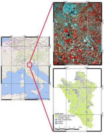
The study area is located at south-east of city of Padova, in the Italian Veneto Region (Figure 1). The area is approximately 11 km in the East-West axis and 16 km in the North-South. The extension of the data polygons is approximately 60 km2. The area is roughly composed of urban areas, grassland, and crop sowable area.
Figure 1. The satellite image (above) and land use map (below) of the study area.
3. MATERIALS AND METHODS
3.1 Satellite images – Sentinel-2
The Sentinel-2A satellite successfully launched on 23 June 2015, is becoming an important image data source for a wide spectrum of applications reaching from agriculture to forestry, environmental monitoring to urban planning. The reason is to be
found in the following sensor features. A combination of different spatial resolutions (10 to 60m) with novel spectral capabilities (e.g., three bands in the ‘red-edge’ which provide key information on the state of vegetation plus two bands in the SWIR) – see Table 1. Wide coverage (swath width of 290 km) and minimum five-day global revisit time (with its twin, Sentinel-2B, to be launched in 2016) (Malenovský et. al., 2012). The satellite's orbit is Sun-synchronous, at 786 km altitude, 98.5° inclination. Temporal resolution is 10 days with one satellite and 5 days with 2 satellites. In this study, the Sentinel-2 satellite data dated on 13th August 2015, is used to assess the three methods for accuracy assessment proposed.
Band
Central Wavelength (nm)
Bandwidth (nm)
Spatial resolution (m)
Band 1 443 20 60
Band 2 490 65 10
Band 3 560 35 10
Band 4 665 30 10
Band 5 705 15 20
Band 6 740 15 20
Band 7 783 20 20
Band 7 783 20 20
Band 8 842 115 10
Band 8A 865 20 20
Band 9 945 20 60
Band 10 1375 30 60
Band 11 1610 90 20
Band 12 2190 180 20
Table 1. Band description of Sentinel-2 sensor.
3.2 Classification methods
Supervised classification considers a set of observations S = {x1, x2, …, xn} - sometimes referred to as features, attributes, variables or measurements - for each sample of an area with known class C. This set is called the training set and is usually determined manually by setting regions of interest (ROI). The classification problem is then to find a good predictor for the class C of any sample of the same distribution (not necessarily from the training set) given observation S (Venables and Ripley, 2002). To find good predictors, various machine learning methods are used. The machine learning methods (MLM) tested in this study are given below:
1. Linear Discriminant Analysis (lda), 2. K-nearest Neighbour (kknn), 3. Random Forests (randomForest), 4. Support Vector Machines (svm), 5. Multi Layered Perceptron (mlp),
6. Multi Layered Perceptron Ensemble (mlpe), 7. CTree (ct),
8. Boosting (b),
9. Logistic Regression (lr).
A brief explanation of each method is given below together with some references for further reading:
- Linear discriminant analysis is similar to principal component analysis, where finding the best linear combination of variables to best explain the data is the goal of the process (Venables and Ripley, 2002).
monotonic decreasing function will work. The number of neighbours used for the "optimal" kernel should be:
[ 2 �+4�+2 �
�+4�] (1)
where: d is the distance and k is the number that would be used for unweighted classification, a rectangular kernel. See (Samworth, 2012) for more details.
- Random forests is a very well-performing algorithm which grows many classification trees. To classify a new object from an input dataset, put the set of observations (S) down each of the trees in the forest. Each tree gives a classification, and we say the tree "votes" for that class. The forest chooses the classification having the most votes (over all the trees in the forest). Each tree is grown with specific criteria, which are thoroughly reported in (Breiman and Cutler, 2015). The main features of the random forests method that makes it particularly interesting for digital image analysis are that it is unexcelled in accuracy among current algorithms, it runs efficiently on large data sets (typical among digital images to have a large number of observations), it can handle thousands of input variables without variable deletion and it gives estimates of what variables are important in the classification. Also generated forests can be saved for future use on other datasets. For more reading (Breiman, 2001; Yu et al., 2011).
- Support vector machines is another popular MLM which has been particularly applied in remote sensing by several investigators (Plaza et al., 2009). It uses hyper-planes to separate data which have been mapped to higher dimensions (Cortes and Vapnik, 1995). A kernel is used to map the data. Different kernels are used depending on the data. In this study, the radial basis function kernel is applied.
- Multi layered perceptron and multi layered perceptron ensemble are two neural networks, differing on the fact that the latter method uses average and voting techniques to overcome the difficulty to define the proper network due to sensitivity, overfitting and underfitting problems which limit generalization capability. A multi layered perceptron is a feedforward artificial neural network model that maps sets of input data onto a set of appropriate outputs. It consists of multiple layers of nodes in a directed graph, where each layer is fully connected to the next. Each node is a processing element with a nonlinear activation function. It utilizes supervised learning called backpropagation for training the network. This method can distinguish data that are not linearly separable (Cybenko, 1989; Atkinson and Tatnall, 1997; Benz et al., 2004).
- CTree uses conditional inference trees. The trees estimate a regression relationship by binary recursive partitioning in a conditional inference framework. The algorithm works as follows: 1) Test the global null hypothesis of independence between any of the input variables and the response (which may be multivariate as well). Stop if this hypothesis cannot be rejected. Otherwise select the input variable with strongest association to the response. This association is measured by a p-value corresponding to a test for the partial null hypothesis of a single input variable and the response. 2) Implement a binary split in the selected input variable. These steps are repeated recursively (Hothorn et al., 2006).
- Boosting consists of algorithms which iteratively finding learning weak classifiers with respect to a distribution and adding them to a final strong classifier. When they are added, they are typically weighted in some way that is usually related to the weak learners' accuracy. In this study, the AdaBoost.M1 algorithm is used (Freund and Schapire, 1996).
- Logistic regression method is also being applied in remote sensing data classification (Cheng et al., 2006). It fits multinomial log-linear models via neural networks.
3.3 Classification
Our total dataset consists in approximately 60 km2 therefore, taking as measuring unit the pixel size 10 x 10 m, 6x105 pixels. For each pixel we have information on its land-cover class due to manual interpretation which was provided as polygons with land-cover classes (Figure 1 – bottom left). Because the study requires numerous runs with different combinations of MLM and size of training data, to limit computation time while keeping statistic robustness, we took a smaller subset of the total number of pixels. Pseudo-random stratified sampling was used to choose 20% of the pixels, which gave us 1.2x105 pixels with known classes to work with, hereafter defined as our control dataset. The sampling is “pseudo-random stratified” because two criteria were used to pick “cleaner” pixels. The first criterion consists in choosing only pixels falling completely in a polygon, i.e. no pixels are shared between polygons, thus theoretically decreasing spectral mixing in our control. The second criterion consists in balancing numerosity of pixels per class to avoid having under-represented classes.
The training is then done automatically for each MLM also with stratified random sampling of the control dataset obtained with the aforementioned procedure. Thirty training subsets are picked for each MLM subsetting from 1% to 50% (1200 to 6x104 pixels). The same procedure described above is also carried out over a much smaller subset consisting of 4% of the total dataset pixels. This further processing was done to see the impact of a smaller dataset on results, and results are reported as blue points and red points, on figures 2 and 3, for 4% and 20% respectively.
3.4 Validation
The control dataset consists of an independent classification with 11 land-cover classes in the total area (see Figure 1). The class attribution was done by manual visual interpretation of high resolution images (20 cm ground sampling distance) by experts. In this study, only five out of the eleven classes are used since the other classes cover very small areas with the consequence that the samples (pixels) for testing and validating subsets are not frequent enough to be tested significantly. The classes used are the following: (i) urban, (ii) sowable areas, (iii) water, (iv) tree plantations, and (v) grasslands.
Five accuracy indices are calculated:
- Classification accuracy rate (ACC) [0-100] - Classification error (CE) [0-100]
- Balanced error rate (BER) [0-100] - Kappa index (KAPPA) [0-100] - Cramer's V (CRAMERV) [0-1]
4. RESULTS AND DISCUSSION
As reported in the previous section, validation has been done using three sets of data. The validation against the training set (train) is not reported in a figure, because it is not cross-validated in any way and not independent. As a matter of fact, as expected, the accuracies from train validation were much over-estimated when compared to the other methods; i.e. for one of the MLM method, RF, the accuracy was 100%, as the decision trees model the training data perfectly (with decisions) and thus validation against training does not have any sense.
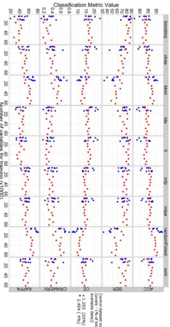
The k-fold cross-validation and the validation against the full dataset are reported in Figure 2 and Figure 3, respectively.
Figure 2. Accuracy metrics of k-fold cross validation over the training set.
4.1 Best performing classifier
The first question that needs to be asked is: what is the best classifier? As can be seen in Figure 2, the random forests (RF) performs better than the others, however there are several points that should be made. First of all, RF keeps the title of “best performer” when there are enough training variables. As can be
seen in both plots, below 20 x103 pixels for training RF tends to be as accurate, if not less, than other MLM.
The two MLM based on neural networks (MLP and MLPE) seem to perform better than RF when considering smaller number of pixels for training. This is particularly clear from the validation results from the full independent dataset (Figure 3), where RF drops. RF also gets the title of best performer when comparing accuracies with the k-fold cross validation, keeping the title also at lower number of training pixels.
Figure 3. Accuracy metrics of results over the full independent dataset.
4.2 K-fold versus full validation
K-fold does have a small drawback when compared against validation from the full dataset. It overestimates accuracy when using the 2% of total polygons (blue dots) as opposed to the 10% of total polygons (red dots). This is explained by the smaller set used for training when using 2% of the available pixels as opposed to 10%. K-fold cross-validation uses available training data to assess accuracy, simulating independent sets of data by sampling from the training data and applying the model to it. Therefore, a smaller set will overestimate accuracy as opposed to a larger training set, which has more variance. It is trivial to state that validation against the full dataset is more robust. This type of overestimation of accuracy is observed in RF and KKNN, but not in the other classifiers.
4.3 Processing speed
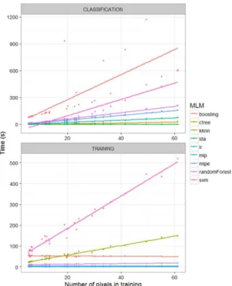
Each combination of MLM and number of pixels used for training were also benchmarked for its speed in processing (Figure 4). This benchmark was performed by running the MLMs with R cran rminer package (Cortez, 2010) on a workstation with 1 Intel® Xeon® Six-Core Processor X5660 (2.80 GHz, 12 MB cache, 1333 MHz memory), 12 Gb RAM running Windows©7 64 bits.
Figure 4. Benchmark results of processing speeds for each MLM with different number of pixels used in the training phase.
Figure 5. Processing speed of different MLMs for training and classification using the highest number of pixels for training (6x10⁴).
This type of benchmark is to be considered for testing relative performance issues between MLMs in this particular case, and not an indicator for a final conclusion on speed of the algorithms as they are influenced by many factors which have not been monitored in this study.
As shown n Figure 5, a group of classifiers are much faster in the training phase, especially when the highest number of training pixels – i.e. 6x104 pixels, are used. In training, the faster MLMs are lda, lr, ctree, and mlp. In the classification phase only boosting and kknn, followed by ctree, are significantly faster. The more complex methods, randomForest and svm, require longer processing times for both classification and training.
5. CONCLUSIONS
In this study, the benchmarking of 9 machine learning algorithms is carried out for accuracy and speed in training and classification of a Sentinel-2 dataset for land-cover mapping. Some interesting points which are worth reporting are outlined as below: - Overall, the RF is among the best performing method for the
classification, i.e., Kappa index ranging from 0.55 to 0.42 respectively with the most and least number pixels for training. - Next, the neural networks (mlp and mlpe) follow closely to randomForest and also have an important added value of keeping a high accuracy with smaller training datasets, as opposed to randomForest, i.e., drops in accuracy with a smaller number of training data.
- The support vector machines also follow close, and it can be said that there are various methods to improve performance of SVM which have not been investigated in this study. - Although many factors which have not been monitored in this
study, affect the speed of the algorithms used, in general, the more complex methods, such as randomForest and svm, showed that they require longer processing times for both classification and training phases.
6. REFERENCES
Akın, A., Sunar, F., Berberoğlu, S., 2015. Urban change analysis and future growth of Istanbul
,
Environmental Monitoring and Assessment, 187(8), 1-15.Atkinson, P.M., Tatnall, A.R.L., 1997. Introduction Neural networks in remote sensing. International Journal of Remote Sensing, 18, 699–709.
Benz, U.C., Hofmann, P., Willhauck, G., Lingenfelder, I., Heynen, M., 2004. Multi-resolution, object-oriented fuzzy analysis of remote sensing data for GIS-ready information. ISPRS Journal of Photogrammetry and Remote Sensing. Breiman, L., 2001. Random forests. Machine Learning, 45, 5– 32.
Breiman, L., Cutler, M.E.J., 2015. Random forests [WWW Document].
URL,https://www.stat.berkeley.edu/~breiman/RandomForests/c c_home.htm (accessed 7 November 2015).
Chen, J., Dowman, I., Li, S., Li, Z., Madden, M., Mills, J., Paparoditis, N., Rottensteiner, F., Sester, M., Toth, C., Trinder, J., Heipke, C., 2015. Information from imagery: ISPRS scientific vision and research agenda. ISPRS Journal of Photogrammetry and Remote Sensing.
Cheng, Q.C.Q., Varshney, P.K., Arora, M.K., 2006. Logistic Regression for Feature Selection and Soft Classification of Remote Sensing Data, IEEE Geoscience and Remote Sensing Letters.
Cortes, C., Vapnik, V., 1995. Support-vector networks. Machine Learning, 20, 273–297.
Cortez, P., 2010. Data Mining with Neural Networks and Support Vector Machines Using the R/rminer Tool. 10th Industrial Conference, ICDM 2010, 6171, 572–583.
Cybenko, G., 1989. Correction: Approximation by Superpositions of a Sigmoidal Function. Mathematics of Control, Signals, and Systems, 2, 303–314.
Freund, Y., Schapire, R.R.E., 1996. Experiments with a New Boosting Algorithm. International Conference on Machine Learning, 148–156.
Hothorn, T., Hornik, K., van de Wiel, M. a, Zeileis, A., 2006. A Lego System for Conditional Inference. The American Statistician, 60, 257–263.
Malenovský, Z., H. Rott, J. Cihlar, M. E. Schaepman, G. García-Santos, R. Fernandes, M. Berger, 2012. Sentinels for science: Potential of Sentinel-1, -2, and -3 missions for scientific observations of ocean, cryosphere, and land, Remote Sensing of Environment, Volume 120, P.91–101.
Piragnolo, M., Pirotti, F., Guarnieri, A., Vettore, A., Salogni, G., 2014. Geo-Spatial Support for Assessment of Anthropic Impact on Biodiversity. ISPRS International Journal of Geo-Information, 3, 599–618.
Pirotti, F., 2010. IceSAT/GLAS Waveform Signal Processing for Ground Cover Classification: State of the Art. Italian Journal of Remote Sensing, 13–26.
Pirotti, F., Laurin, G., Vettore, A., Masiero, A., Valentini, R., 2014. Small Footprint Full-Waveform Metrics Contribution to the Prediction of Biomass in Tropical Forests. Remote Sensing, 6, 9576–9599.
Plaza, A., Benediktsson, J.A., Boardman, J.W., Brazile, J., Bruzzone, L., Camps-Valls, G., Chanussot, J., Fauvel, M., Gamba, P., Gualtieri, A., Marconcini, M., Tilton, J.C., Trianni, G., 2009. Recent advances in techniques for hyperspectral image processing. Remote Sensing of Environment, 113, S110–S122.
Samworth, R.J., 2012. Optimal weighted nearest neighbour classifiers. Annals of Statistics, 40, 2733–2763.
Scaioni, M., Longoni, L., Melillo, V., Papini, M., 2014. Remote sensing for landslide investigations: An overview of recent achievements and perspectives. Remote Sensing, 6(10), 9600-9652.
Scarano M., 2015. On the relationship between the urban parameters sky view factor, normalized difference vegetation index and vegetation fraction and the land surface temperature derived by Landsat-8 in Bari, Italy. Bollettino SIFET, 2, pp.1-9. Tarantino E., 2012. Monitoring spatial and temporal distribution of Sea Surface Temperature with TIR sensor data. Italian Journal of Remote Sensing, 44, pp.97-107.
Venables, W.N., Ripley, B.D., 2002. Modern Applied Statistics with S. Issues of Accuracy and Scale, 868.