Radiatively Induced Non Linearity in the Walecka Model
Rafael Cavagnoli∗
Departamento de F´ısica, Universidade Federal de Santa Catarina, 88040-900 Florian´opolis, Santa Catarina, Brazil and
Centro de F´ısica Te´orica - Dep. de F´ısica - Universidade de Coimbra - P-3004 - 516 - Coimbra - Portugal Marcus Benghi Pinto†
Departamento de F´ısica, Universidade Federal de Santa Catarina, 88040-900 Florian´opolis, Santa Catarina, Brazil (Received on 25 August, 2010)
We evaluate the effective potential for the conventional linear Walecka non perturbatively up to one loop. This quantity is then renormalized with a prescription which allows finite vacuum contributions to the three as well as four 1PI Green’s functions to survive. These terms, which are absent in the standard relativistic Hartree approximation, have a logarithmic energy scale dependence that can be tuned so as to mimic the effects ofφ3 andφ4type of terms present in the non linear Walecka model improving quantities such as the compressibility modulus and the effective nucleon mass, at saturation, by considering energy scales which are very close to the nucleon mass at vanishing density.
Keywords: Renormalization; Nuclear matter; Finite densities, Vacuum corrections; Walecka model.
1. INTRODUCTION
Quantum hadrodynamics (QHD) is an effective relativistic quantum field theory, based on mesons and baryons, which can be used at hadronic energy scales where the fundamen-tal theory of strong interactions, quantum chromodynamics (QCD), presents a highly nonlinear behavior. The Walecka model [1] to be considered here represents QHD by means of a Lagrangian density formulated so as to describe nucle-ons interacting through the exchange of an isoscalar vector meson (ω) as well as of a scalar-isoscalar meson (φ) which is introduced to simulate intermediate range attraction due to thes-wave isoscalar pion pairs. The original Walecka model (QHD-I) is described by the Lagrangian density
L
= ψ¯[γµ(i∂µ−gvVµ)−(M−gsφ)]ψ+1 2(∂µφ∂
µφ
−m2sφ2)
− 1
4FµνF
µν+1
2m 2
vVµVµ−U(φ,V) +
L
CT, (1) where ψ, φ and ω denote respectively baryon, scalar and vector meson fields (with the latter being coupled to a con-served baryonic current). The termU(φ,V), which describes mesonic self interactions was set to zero in the original model so as to minimize the many body effects while the termL
CT represents the counterterms needed to eliminate any potential ultra violet divergences arising from vacuum computations.It is important to recall that, roughly, counterterms are composed by two distinct parts the first being a divergent piece which exactly eliminates the divergence resulting from the evaluation of a Green function at a given order in pertur-bation theory. The second piece is composed by a finite part which isarbitraryand can be fixed by choosing an appropri-ated renormalization scheme [2].
The important parameters are the ratios of coupling to masses,C2s andCv2, withCi2= (giM/mi)2which are tuned to
∗Electronic address:[email protected] †Electronic address:[email protected]
fit the saturation densityρ0=0.193 fm−3and binding energy per nucleon,BE =−15.75 MeV [1]. However, the QHD-I predictions for some other relevant static properties of nu-clear matter do not agree well with the values quoted in the literature. For example, using the Mean Field Approxima-tion (MFA) which considers only in medium contribuApproxima-tions at the one loop level one obtains that, at saturation, the ef-fective nucleon mass isMsat∗ ∼0.56M, which is somewhat low, while the compression modulus,K∼540 MeV, is too high according to the accepted values in the literature [3–5]: Msat∗ /M∼0.70 to 0.80 andK∼200 MeV to 300 MeV. Let us point out that the effective nuclear mass at saturation density is not known accurately. According to the type of data and its analysis, the effective mass is defined in different ways, and so this mass usually is not that of the nuclear field theory, although they might be close and related to each other.
In principle, since this is a renormalizable quantum field theory, vacuum contributions (and potential ultra violet di-vergences) can be properly treated yielding meaningful fi-nite results. These contributions were first considered by Chin [6], at the one loop level, in the so called Relativistic Hartree Approximation (RHA) which produced a more rea-sonable value for the effective mass,M∗sat∼0.72M. How-ever, the compression modulus remained at a high value, K∼470 MeV.
One could then try to improve the situation by also con-sidering exchange contributions since both, MFA and RHA, consider only direct terms in a nonperturbative way. When vacuum contributions are neglected this approximation is known as the Hartree-Fock (HF) approximation producing Msat∗ ∼0.53M and K∼585 MeV [1]. By comparing the results from MFA, RHA and HF one sees how vacuum ef-fects can improve the values ofMsat∗ andK. Then, the natural question is if the situation could be further improved by con-sidering the vacuum in HF type of evaluations. The main concern now being the difficulty to deal with overall, nested, and overlapping type of divergences which surely arise due to the self consistent procedure.
which only the propagators have been fully renormalized ). This cumbersome calculation considers the nonperturbative evaluation and renormalization of the energy density up to the two loop level showing the non convergence of the loop expansion. Later, the situation has been addressed with the alternative Optimized Perturbation Theory (OPT) which al-lows for an easier manipulation of divergences [9]. Two loop contributions have been evaluated and renormalized in a per-turbative fashion with nonperper-turbative results further gener-ated via a variational criterion. However, saturation of nu-clear matter could not be achieved with the results supporting those of Ref. [7].
Meanwhile, the compressibility modulus problem has been circumvented by introducing some more parameters, in the form of new couplings [10], to the original Walecka model. One then considersU(φ,V)appearing in Eq. (1) as
U(φ) = κ
3!φ 3+ λ
4!φ 4,
(2) whereκ=2bMg3s andλ=6cg4s. This version of QHD is known as the nonlinear Walecka model (NLWM) and the main role of the two additional parameters, b andc, is to bring the compression modulus of nuclear matter and the nucleon effective mass under control. However, one may object to this course of action since the mesonic self inter-actions will increase the many body effects apart from in-creasing the parameter space. Notice also that terms likeφn
(n≥5) are not allowed since then, in 3+1 dimensions, one would need to introduce coupling parameters with negative mass dimensions spoiling the renormalizability of the origi-nal model apart from increasing the parameter space.
Heide and Rudaz [11] have then realized that it is still pos-sible to keepU(φ,V) =0 while improving bothKandMsat∗ . The key ingredient in their approach is related to the com-plete evaluation (regularization and renormalization) of di-vergent vacuum contributions. Regularization is a formal way to isolate the divergences associated with a physical quantity for which many different prescriptions exist, e.g., sharp cut-off, Pauli-Villars, and Dimensional Regularization (DR). Within DR, which was used by Chin, one basically performs the evaluations ind−2εdimensions takingε→0 at the end so that the ultra violet divergences show up as powers of 1/ε. However, to keep the dimensionality right when doingd→d−2εone has to introducearbitraryscales with dimensions of energy (Λ, or the related1 Λ
MS). Chin has chosen a renormalization prescription in which the fi-nal results do not depend on the arbitrary energy scale while Heide and Rudaz chose one in which such a dependence re-mains, as in most QCD applications. Since the latter au-thors also worked at the one loop level their approximation became known as the Modified Relativistic Hartree Approx-imation (MRHA) and their main result was to show that it is possible to substantially improveK andM∗sat by suitably fixing the energy scale,Λ. Moreover by choosingΛ=Mthe MRHA recovers RHA. In connection with neutron stars, the
1The relation between both scales is given by a constant term,Λ MS=
√
4πe−γEΛ, whereγE=−0.5772....
MRHA has been applied to the Walecka model in Refs. [12]. The dependence of QHD results on the choice of renormal-ization conditions, which may be expected in phenomeno-logical models, has been shown long ago (see Ref. [13] and references therein). At the same time, it has been discussed that approximations of the pure Walecka model are incon-sistent leading to an unstable ground state [14] and ignoring the usual nonlinear contributions due to renormalization car-ries the danger to reenter this instability also in the quantum corrected Walecka model. In principle these facts will spoil any rigorous attempt to include vacuum corrections, in the usual Walecka model, at arbitrarily high orders. Very often however, this model is still being treated at the one loop level with the MFA and the aim of the present paper is to show that in this case the values ofKandM∗satcan be improved simply by evaluating vacuum corrections up to an energy scale very close (but not equal) to the nucleon mass at zero density.
Therefore, even if our procedure may be spoiled at higher orders by the facts mentioned above we believe that for it remains a useful, and easy to implement, procedure which improves MFA results without the need for new paremeters in the theory. This is an important feature to be considered. Secondly, as we shall see, models which lead to low effective masses at saturation are not suitable for neutron stars calcu-lations, another important application of RMF (Relativistic Mean Field) models.
Also, one of our goals is to treat the Walecka model us-ing a formalism which is closely related to the one used in QCD and other modern quantum field theories. Within the QHD model, the temperature and density are usually intro-duced using the real time formalism employed in the orig-inal work of Walecka. Instead, we use Matsubara’s imagi-nary time formalism treating the divergent integrals with DR adapted to the modified minimal subtraction renormalization scheme MS [2] which constitute the framework most com-monly used within QCD. To obtain the ground state energy density, ε, we will first evaluate the effective potential (or Landau’s free energy),
F
, whose minimum gives the pres-sure,P. By choosing appropriate renormalization conditions we generate effective three- and four-body couplings, inF
, which are not present at the classical level. As we shall see the numerical values of these effective couplings run with the energy scale,ΛMS, allowing for a good tuning ofKandM∗sat which have their values improved at energy scales of about 0.92M-0.98M(M=939 MeV) while the usual RHA results are retrieved for the choiceΛMS=M.The MRHA proposed by Heide and Rudaz suggests that if one seeks to minimize many-body effects in nuclear mat-terat saturation, the choiceΛ≃Msat∗ is the necessary one. Our philosophy is slightly different and perhaps simpler to implement. Since possible modifications in the behavior of KandM∗seem to be dictated by the presence ofκeffφ3and λeffφ4type of terms we shall use the Chin-Walecka renor-malization prescription to deal withφn(n=0,1,2) vacuum
onlyκeffandλeffrun withΛMSbut, as we shall see, one also retrieves the RHA atΛMS=M.
Considering the effective potential at zero density we will choose an appropriate renormalization prescription for this particular model. Since our main goal is to improveKand Msat∗ by quantically renormalizing κ=0→κeff(ΛMS)and λ=0→λeff(ΛMS)we can keepM,ms,mvas representingthe
vacuum physical masses for simplicity. This choice means that, atkF=0, all mass parameters (M,ms,mv) represent the
effective vacuum masses and shall not run withΛMSas op-posed to κeff andλeff. In theories such as QCD the run-ning of the couplings is dictated by the β function whose most important contributions come from the so-called lead-ing logs, e.g. ln(ΛMS/M), which naturally arise in DR evalu-ations. The application of renormalization group (RG) equa-tions to the effective Walecka model is beyond the scope of our work2. Nevertheless, our renormalization prescription to obtain a scale dependence so as to better controlK and Msat∗ is inspired by the leading logs role in theβfunction and the the renormalization scheme presented here proposes that one should preserve only the scale dependent leading logs which appear in the expressions forκeffφ3andλeffφ4. As a byproduct, and contrary to the MRHA case, both quantities will display the same scale dependence. Here, this approx-imation will be called the Logarithmic Hartree Approxima-tion (LHA). The numerical results show that the best LHA predictions forKandMsat∗ according to the literature are ob-tained at energy scales which are only about 5% smaller than that of the RHA, that isΛMS≃0.95M. This is a nice feature since the values of the energy scale and that of the highest mass in the spectrum are almost the same whereas in the MRHA the optimum scale, set to be close toMsat∗ is about 35% smaller thanM. From the quantitative point of view, the LHA produces better results than the MRHA as will be shown.
The work is presented as follows. In the next section the one loop free energy is evaluated using Matsubara’s formal-ism. The renormalization of the vacuum contributions is dis-cussed in Section III and the complete renormalized energy density is presented in Section IV. Numerical results and dis-cussions appear in Section V while our conclusions are pre-sented in Section VI. For completeness, in the appendix, we discuss a case in which ms does not represent the physical
mass.
2. THE FREE ENERGY TO ONE LOOP
In quantum field theories the effective potential (or Lan-dau’s free energy),
F
, is defined as the generator of all one particle irreducible (1PI) Green’s functions with zero exter-nal momentum. The standard textbook definition (for one field,φ) reads [2]F
(φc) = ∞∑
n=0˜
Γ(n)(0)φnc, (3)
2See Ref. [16] for a RG investigation of the Walecka model.
where we have absorbed non relevant factors ofiandn! by defining ˜Γ(n)(0) = (−i)nΓ(n)(0)/n! with Γ(n)(0)
represent-ing the 1PIn-point Green’s function andφcrepresenting the
classical (space-time independent) scalar field. In practice, this quantity incorporates quantum (or radiative) corrections to the classical potential which appears in the original La-grangian density. While the latter is always finite the for-mer can diverge due to the evaluation of momentum integrals present in the Feynman loops. One way to obtain this free energy density is to perform a functional integration over the fermionic fields [2]. To one loop this leads to
F
(φc,Vc) =− m2v2 Vc,µV
µ c +
+ m
2 s
2 φ 2 c+i
Z d4k
(2π)4tr ln[γ µ(k
µ−gvVc,µ)−(M−gsφc)](4).
Notice that this free energy density contains the classical potential (zero loop or tree level term) present in the La-grangian density plus a one loop quantum (radiative) cor-rection represented by the third term. Working in the rest frame of nuclear matter we assume that the classical fields are time-like(Vc,µ=δµ,0Vc,µ). Then, after taking the trace
one can write the free energy as
F
(φc,Vc,0) =− m2v2 V 2 c,0+
m2s 2 φ
2 c+iγ
Z d4k
(2π)4× ×ln[−(k0−gvVc,0)2+k2+ (M−gsφc)2], (5)
whereγ=4(2)is the spin-isospin degeneracy for nuclear (neutron) matter. To obtain finite density results one may use Matsubara’s imaginary time formalism withk0→i(ωn− iµ) where µ represents the chemical potential while, for fermions, ωn= (2n+1)πT (n=0,1, ...) is the Matsubara
frequency withT representing the temperature. Then, upon using
Z d4k
(2π)4→iT
∑
nZ d3k
(2π)3, (6)
the free energy reads
F
(φc,Vc,0) =− m2v2 V 2 c,0+
m2s 2 φ
2 c−γT
∑
n
Z d3k
(2π)3× ×ln{[ωn−(µ−gvVc,0)]2+k2+ (M−gsφc)2]. (7)
The Matsubara’s sums can be performed using
T
+∞
∑
n=−∞ln[(ωn−iµ′)2+E2] =E+
Tlnh1+e−(E+µ′)/Ti+Tlnh1+e−(E−µ′)/Ti, (8)
whereE2(k) =k2+ (M−g
tempera-ture limit of Eq. (8) which is given by3
lim
T→0T
+∞
∑
n=−∞ln[(ωn−iµ′)2+E2(k)] =E(k) +
+
µ′−E(k)
θ(µ′−E(k)) =max(E(k),µ′). (9) Then, atT =0 andµ6=0, the one loop free energy for the Walecka model becomes
F
(φc,Vc,0) =− m2v2 V 2 c,0+
m2s 2 φ
2 c−γ×
Z d3k
(2π)3
µ′−E(k)
θ(µ′−E(k)) +∆(φc), (10)
where
∆(φc) =−γ Z d3k
(2π)3E(k). (11)
Power counting shows that ∆(φc) is a divergent quantity
while the µdependent term of Eq. (10) is convergent due to the Heaviside step function.
3. THE RENORMALIZED VACUUM CORRECTION
TERM
In order to renormalize the vacuum correction term one must first isolate the divergences which is formally achieved by regularizing the divergent integral. Here we use DR per-forming the divergent integrals in 2ω=3−2εdimensions. Then, in order to introduce the MS energy scale,ΛMS, com-monly used within QCD one redefines the integral measure as
Z d3k
(2π)3→
eγEΛ2 MS 4π
!ε/2
Z d2ωk
(2π)2ω , (12)
whereγE=−0.5772...represents the Euler-Mascheroni
con-stant. Note that, with this definition, irrelevant factors of γE and 4π are automatically canceled but the results of
Refs. [6, 9, 11] can be readily reproduced by usingΛMS=
√
4πe−γEΛ. The integral can then be performed yielding [2]
∆(φc) =γ
(M−gsφc)4
32π2
1
ε+
3 2−2 ln
(M
−gsφc)
ΛMS
.
(13) As one can see, by expanding the the term proportional to 1/ε, there are five potentially divergent contributions ranging fromg0tog4while all terms of ordergn(n≥5) are conver-gent. The divergent terms proportional toΓ(n)φn
c(n=0, ...,4)
are respectively ˜
Γ(0)=γ M 4 32π2 1 ε+ 3 2−2 ln
M ΛMS
, (14)
3As discussed in Ref. [15] this procedure must be taken with care if one
includes loop corrections to the meson propagators which is not the case here.
˜
Γ(1)φc=−γ gsφcM3
8π2
1
ε+1−2 ln
M ΛMS , (15) ˜
Γ(2)φ2c=γ
3(gsφc)2M2
16π2
1
ε+
1 3−2 ln
M ΛMS , (16) ˜ Γ(3)φ3
c=−γ
(gsφc)3M
8π2
1
ε−
2 3−2 ln
M ΛMS , (17) and ˜ Γ(4)φ4
c=γ (gsφc)4
32π2
1
ε−
8 3−2 ln
M
ΛMS
. (18)
The counterterms contained in
L
CT needed to render the free energy finite are [6, 9]L
CT=4
∑
n=0αn n!φ
n
c, (19)
where theαncoefficients have the general form
αn∼gns
1
ε+fn(ΛMS)
. (20)
Now, within the MS renormalization scheme generally adopted within QCD one simply sets fn=0 and the
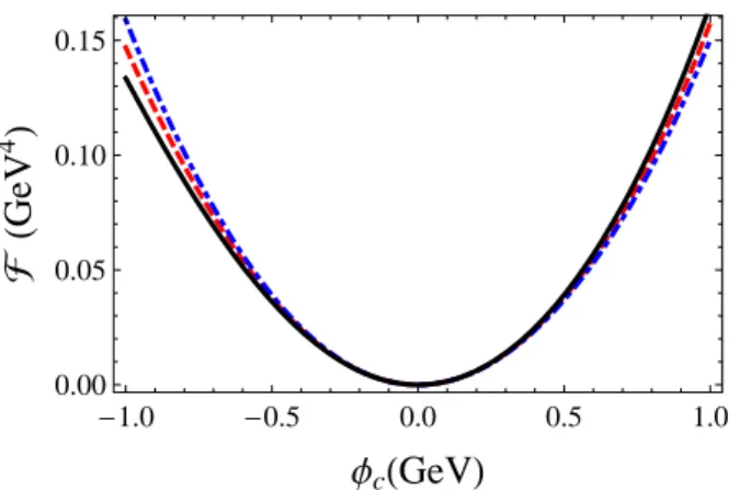
coun-terterms have only the bare bones needed to eliminate the 1/εpoles while the final finite contributions depend on the arbitrary energy scale. If one adopts this scheme within the Walecka model the free energy would look like the dashed curve in Fig. 1 which shows
F
versusφc for the values4ΛMS=0.9 GeV, M =1 GeV, ms=0.55 GeV, and gs=1.
As it is well known, within this schemeM,ms, andmv do
not represent the measurable physical vacuum masses which are instead taken as mass parameters whose values, like the values of the couplings, run withΛMS in a way ultimately dictated by RG equation.
If instead, like Chin, one adopts the so-called on-mass renormalization scheme the counterterms completely elim-inate the total contributions represented by Eqs (14-18). Within this choice the results are scale independent whileM, ms, andmvrepresent the measurable physical masses at zero
density whereas the three and four-body mesonic couplings vanish in agreement with the tree level result displayed by the original Lagrangian density. The free energy generated by this scheme is represented by the dashed line in Fig. 2. Considering the relevantkF=0 case, let us find a hybrid
al-ternative scheme between the MS and the on-mass-shell so that a residual, scale dependent, contribution survives within the three and four 1PI Green’s function given by Eqs (17) and (18).
1.0 0.5 0.0 0.5 1.0 0.00
0.02 0.04 0.06 0.08 0.10 0.12 0.14
Φ
cGeV
GeV
4
FIG. 1: (color online) The free energy, in the φcdirection, as a
function of the classical field forΛMS=0.9 GeV,M=1 GeV,ms=
0.55 GeV, andgs=1. The dashed line is the MS renormalization
scheme result. The dotted-dashed corresponds toΓ(0)=Γ(1)=0
while MS is used in the remaining three 1PI function. The same situation but withΓ(2)=0 is represented by the dotted line. The
continuous line represents the LHA prescription.
1.0 0.5 0.0 0.5 1.0
0.00 0.05 0.10 0.15
Φ
cGeV
GeV
4
FIG. 2: (color online) The free energy, in the φcdirection, as a
function of the classical field forΛMS=0.9 GeV,M=1 GeV,ms=
0.55 GeV, andgs=1. All curves represent the LHA prescription at
the different scalesΛMS=0.9 GeV<M(continuous line),ΛMS=
1 GeV=M(dashed line) andΛMS=1.1 GeV>M. The dashed line also corresponds to the RHA result.
To do that, let us analyze each of the arbitrary fn terms
contained in the counterterm coefficients from the physical point of view starting with f0which is contained in the field independentΓ(0). This contribution is renormalized by the
constant countertermα0which can be referred to as the “cos-mological constant” [17]. In practice, the only effect this term has is to give the zero point energy value and by its complete elimination one assures that
F
(φc=0) =0 which,within the Walecka model, will later assure that the pressure as well as the energy density vanish atkF=0. Therefore,
as in the on-mass shell prescription, we can impose that f0 be exactly equal to the finite part of theΓ(0) term. It is
im-portant to point out that even if one uses the MS scheme this term can be absorbed in a vacuum expectation value subtrac-tion of the zero point energy so that the exact way in which it done is not too relevant for the present purposes.
The effect of the the linear (tadpole) termΓ(1)φ
cis to shift
the origin so that the minimum is not at the origin ( ¯φc6=0)
as shown by the dashed line of Fig. 1. Also any finite contri-bution left in the tadpole will cause direct terms to contribute to the baryon self energy which, at the present level of ap-proximation, means thatM does not represent the physical nucleon mass atkF =0, M∗vac. This can be understood by recalling that the baryon self-energy isΣB∼gsΓ˜(1)(ΛMS)so that the vacuum effective baryon mass is given byM∗vac=
M+ΣB(ΛMS)and since Mvac∗ =939 MeV one sees thatM, as well as gs and ms, should depend on ΛMS. However, for the purposes of controllingKandM∗satthe renormaliza-tion of the baryonic vacuum mass fromM toMvac∗ does not generate the wantedφ3andφ4vertices. Therefore, for sim-plicity, we can also set f1so as to completely eliminate the tadpole vacuum contribution. This choice for f0and f1 to-gether with f2= f3= f4=0 produces the dot-dashed line of figure 1. The termΓ(2)represents a (momentum
indepen-dent) vacuum correction to the scalar meson mass,ms. As in
the previous case, getting rid of this term assures thatmsbe
taken as the physical mass simplifying the calculations since
(m∗s,vac)2=m2
s+Σs(ΛMS) whereΣs(ΛMS)∼g2sΓ˜(2)(ΛMS). Fixing f2 so as to completely eliminate the Γ(2)
contribu-tion produces the dotted line of figure 1. In summary, so far we have adopted the usual Chin-Walecka on-mass shell renormalization conditions for f0,f1, and f2so that: the vac-uum energy is normalized to zero,φc=0 is the minimum
of
F
(also meaning thatM=Mvac∗ ), whilemsrepresents thevacuum scalar meson mass. In this approach, none of the vacuum mass parameters present in the original Lagrangian density run withΛMS. Note that, physically, our choice was also inspired by the NLWM observation that the compress-ibility modulus is improved by the introduction ofφ3andφ4 terms which is consistent with our choice of neglecting any corrections to terms proportional toφ2andφψψ¯ which are re-spectively related with the scalar meson and baryon masses.
Now, taking f3=0 and f4=0 would leave us with the wantedφ3andφ4scale dependent terms. However, inspec-tion of Eq. (17) and Eq. (18) shows that these contribu-tions would vanish at different scales, given byΛMS=Me1/3 andΛMS=Me4/3respectively. As already emphasized the NLWM controls the compression modulus with theκφ3and λφ4terms so one can impose that, within our approach, both κeff and λeff arise at the same energy scale. This can be achieved by imposing thatΓ(3) =Γ(4) =0 atΛ
dependent, vacuum contribution is then given by ∆LHA
R (φc,ΛMS) =− γ 16π2
(M−gsφc)4ln
M
−gsφc M
+ gsφcM3−
7 2(gsφc)
2M2+13 3 (gsφc)
3M −25
12(gsφc) 4
+ γ
4π2
(gsφc)3M−
1 4(gsφc)
4 ln M ΛMS . (21)
The free energy obtained with this finite vacuum contribu-tion term is shown in Fig 2 forΛMS<M (continuous line), ΛMS>M(dot-dashed line) as well as forΛMS=M(dashed line) in which case the usual RHA is retrieved. As one can check, the first term in Eq. (21) is just the RHA vacuum correction [6] so that, in view of Eq. (2), one can write
∆LHAR (φc,ΛMS) =∆ RHA R (φc) +
κeff 3! φ 3 c+ λeff 4! φ 4
c , (22)
whereκeff=2g3sMbeff(ΛMS)andλeff=6g4sceff(ΛMS)with
beff(ΛMS) = 3 π2ln
M
ΛMS
(23)
and beff(ΛMS) =−3ceff(ΛMS). In this way not only κeff and λeff vanish at the same scale but an inversion of their respective signs happen at the same time. We have then achieved our goal by quantically inducingκ=0→κeff(ΛMS) andλ=0→λeff(ΛMS)in a way that all the scale depen-dence is contained in the leading logs and also achieving κeff(ΛMS) =λeff(ΛMS) =0 atΛMS=M.
For comparison purposes let us quote the MRHA result
∆MRHAR (φc,Λ) = ∆RHAR (φc) +γ (gsφc)3
4π2 ln M Λ −1 + Λ M
−γ(gsφc) 4
16π2 ln
M Λ
. (24)
One notices that the major difference between the MRHA and our prescription amounts to the finite contribution con-tained within the cubic term where the scale dependence is
not restricted to the leading log being also contained in an ex-tra linear term which does not naturally arise when expands the DR results for the loop integrals in powers ofε, as shown by Eqs. (14-18).
4. RENORMALIZED ENERGY DENSITY
To obtain the thermodynamical potential, Ω, one mini-mizes the free energy (or effective potential) with respect to the fields. That is,Ω=
F
(σ¯c,V¯0) =−P, wherePrepresents the pressure. Then, the LHA renormalized pressure isPLHA = m
2 v
2 V 2 c,0−
m2s 2 φ¯
2 c+γ
Z kF
0 d3k (2π)3
×
(µ−gvV0,c)−E∗(k)−∆LHAR (φ¯c,ΛMS)(25)
where E∗= (k2+M∗)1/2 with M∗=M−gsφ¯c while the
Fermi momentum is given byk2F= (µ−gvV0,¯ c)2−M∗2. For
the vector field one gets
V0,c= gv m2 v
ρB, (26)
whereρB= (γk3F)/(6π2)is the baryonic density whereas for
the scalar field the result is
¯ φc=
gs m2
s
[ρs+∆′RLHA(φ¯c)], (27)
where
ρs=γ M∗ 2π2
Z kF
0
dk k 2
E∗(k), (28)
represents the scalar density and
∆′RLHA(φ¯c) = −
γ 4π2
M∗3ln
M∗ M
+gsφ¯cM2−
5 2(gsφ¯c)
2M+11 6 (gsφ¯c)
3
+ γ
4π2
3(gsφ¯c)2M−(gsφ¯c)3
ln M ΛMS . (29)
To get the energy density, ε, one can use the relationε=
−P+µρBobtaining
εLHA= g2v
2m2 v
ρ2 B+
m2s 2 φ¯
2 c+
γ 2π2
Z kF
0
× k2dkE∗(k) +∆LHAR (M∗,ΛMS), (30)
∆LHA
R (M∗,ΛMS) = − γ 16π2
M∗4ln
M∗
M
+ (M−M∗)M3−7 2(M−M
∗)2M2
+ 13
3 (M−M
∗)3M−25 12(M−M
∗)4
+ γ
4π2
(M−M∗)3M−1 4(M−M
∗)4
ln
M ΛMS
, (31)
and
M∗=M−γg 2 s m2
s M∗ 2π2
Z kF
0 k2 E∗(k)dk−
g2s m2 s
∆′R(M∗,ΛMS),
(32)
where
∆′RLHA(M∗,ΛMS) = − γ 4π2
M∗3ln
M∗
M
+ (M−M∗)M2−5 2(M−M
∗)2M+11 6 (M−M
∗)3
+ γ
4π2
3(M−M∗)2M−(M−M∗)3
ln
M ΛMS
. (33)
5. NUMERICAL RESULTS
Let us now investigate the numerical results furnished by LHA for the baryon mass at saturation as well as for the com-pressibility modulus, with the latter given by
K=
k2∂ 2
∂k2
ε
ρB
k=kF
=9
ρ2 B
∂2 ∂ρ2
B
ε
ρB
ρB=ρ0 . (34)
Table I shows the coupling constants and saturation proper-ties for some values of the renormalization scale (ΛMS) that yieldBE=−15.75 MeV andkF=1.42 fm−1(280.20 MeV).
These values are chosen just in order to compare with the original Walecka Model (QHD-I) [1]. The meson masses are ms=512 MeV andmv=783 MeV. This table shows that
some of the best LHA values are obtained withΛMSvalues which are very close toM. Since atΛMS=Mthe RHA re-sult is reproduced one concludes, based on our rere-sults, that a slight decrease from the RHA energy scale produces an enormous effect on the values of both,KandM∗sat.
Figures 3 (a) and (b) show the binding energy per baryon, BE=E/A−M, and the effective baryon mass as functions of the Fermi momentum for someΛMSvalues, shown in ta-ble I. One easily sees the effect of considering the vacuum contribution and its improvements on the compressibility and the effective mass. As expected, whenΛMS=M, the RHA results are recovered. From figures 4 (a) and (b) it is possible to see some properties obtained in table I within the LHA ap-proach, as functions ofΛMS/M. One notes from figure 4 (a) that whenΛMSincreases the value of the nuclear compress-ibility (K) also increases andM∗sat decreases. The crossing point in figure 4 (a) represents the RHA values ofKandM∗ which occurs when we setΛMS=M. Figure 4 (b) shows the
effective couplings that arise due to the LHA as functions of ΛMS/M. Similarly whenΛMSreaches the valueMthe RHA results are recovered and the effective couplings vanish.
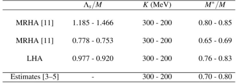
To compare our numerical results with those provided by the MRHA let us make a remark concerning the ef-fective nucleon mass. From a non-relativistic analysis of scattering of neutron-Pb nuclei it has been found [3] that Msat∗ /M≈0.74 to 0.82 which can be viewed as approxi-mately describing the Landau effective mass [4]. The rela-tivistic isoscalar component known as the effective mass de-fined in Eq. (32) can be called the Dirac effective mass and is related to the Landau effective mass. Therefore, the range ex-pected for the Dirac effective mass at saturation density lies in the rangeMsat∗ /M≈0.70 to 0.80 whereas for the nuclear compressibility at saturation the most widely accepted values areK≈200 MeV to 300 MeV [5]. For this range ofKand ac-cording to table II the MRHA predictsMsat∗ /M≈0.80 to 0.85 forΛ/M≈1.185 to 1.466. However, one should note that this MRHA energy scale range is not unique and can also be reproduced withΛ/M≈0.753 to 0.778 which in turn leads to a rather low range forMsat∗ values,Msat∗ /M≈0.65 to 0.69. Our results, shown in tables I and II, seem to produce a bet-ter agreement for this range of K giving the uniquerange Msat∗ /M≈0.76 to 0.83 forΛMS/M ≈0.920 to 0.977 with κeff>0 andλeff<0.
As a last remark we would like to point out that if one choosesΛMS/M=0.9805, (gs/ms)2=9.468 fm2 and (gv/mv)2 =4.879 fm2 the LHA approach reproduces the
same saturation properties as performed by the so-called GM2 parameter set according to [18]: K =300 MeV, Msat∗ /M=0.78, BE =−16.3 MeV, kF =1.313 fm−1 and
TABLE I: Coupling constants and saturation properties for some values of the renormalization scale (ΛMS) that yieldBE=−15.75 (MeV) andkF=1.42 fm−1. The meson masses arems=512 MeV andmv=783 MeV. The constantsCsandCvare defined as:Ci= (giM/mi)
.
ΛMS/M K(MeV) Msat∗ /M C2v C2s g2v g2s κeff/M λeff 1.030 1279.408 0.606 171.339 176.984 119.138 52.619 -6.859 49.753 1.020 910.234 0.646 151.744 184.093 105.512 54.736 -4.875 36.063 1.010 639.833 0.684 132.232 185.875 91.945 55.263 -2.485 18.474 1.005 542.279 0.702 123.626 185.609 85.961 55.184 -1.243 9.233
1.000 468.140 0.718 114.740 183.300 79.782 54.497 0.000 0.000
0.990 371.437 0.745 99.784 177.933 69.383 52.901 2.351 -17.099 0.980 314.086 0.767 88.623 173.525 61.622 51.591 4.551 -32.689 0.975 294.260 0.776 84.456 172.456 58.725 51.273 5.651 -40.463 0.970 277.989 0.784 80.307 170.683 55.840 50.746 6.694 -47.684 0.960 253.249 0.798 73.691 168.648 51.240 50.141 8.811 -62.391 0.950 235.660 0.809 67.923 166.440 47.229 49.484 10.855 -76.356 0.940 222.493 0.818 63.025 164.576 43.824 48.930 12.875 -90.058 0.920 202.507 0.832 55.411 162.702 38.529 48.373 17.054 -118.611 0.900 188.175 0.843 49.467 161.826 34.396 48.112 21.375 -148.267
0.8595 166.351 0.8595 40.936 164.038 28.464 48.770 31.349 -218.926
0.850 162.638 0.863 39.348 165.080 27.360 49.080 33.971 -237.992 0.800 144.532 0.876 32.511 172.680 22.606 51.340 49.902 -357.552 0.700 118.409 0.893 23.328 200.551 16.221 59.626 99.833 -770.891 0.600 98.285 0.905 17.052 256.570 11.857 76.281 206.893 -1806.98 0.500 81.019 0.914 12.239 397.387 8.510 118.147 541.142 -5881.97 0.400 65.319 0.921 8.235 1290.240 5.726 383.600 4185.070 -81967.5
(RHA) 468.140 0.718 114.740 183.300 79.782 54.497 -
-(MFT) 546.610 0.556 195.900 267.100 136.210 79.423 -
-−20 −10 0 10 20 30 40 50
0 50 100 150 200 250 300 350 400 450 500
E/A − M (MeV)
kF (MeV)
MFT RHA
(a) Λ
MS = 1.00 M
(b) Λ
MS = 0.90 M
(c) Λ
MS = 0.70 M
(d) Λ
MS = 0.40 M
(a) (b)
(c)
(d)
0 0.2 0.4 0.6 0.8 1
0 200 400 600 800 1000
M
* /M
kF (MeV) MFT
RHA
(a) Λ
MS = 1.00 M
(b) Λ
MS = 0.90 M
(c) Λ
MS = 0.70 M
(d) Λ
MS = 0.40 M
(a) (b) (c) (d)
(a) (b)
FIG. 3: (a)Binding energy per nucleon as a function of the Fermi momentum for different values of our scaleΛMS. We also plot the MFT and RHA results for comparison purposes. The saturation properties are:BE=−15.75 MeV andkF=1.42 fm−1(280.20 MeV).(b)
Similar as figure (a) but for the effective baryon massM∗as a function of the Fermi momentum for different values of the scale. Note that whenΛMS=1 we reproduce the RHA results.
In the appendix we show that leaving a leading log depen-dence also in the two point Green’s function,Γ(2), only
in-creases the numerical complexity without producing results better than the ones generated by the simplest LHA version employed so far.
6. CONCLUSIONS
We have considered the simplest form of the Walecka model to analyze how the values of the compressibility
mod-ulus as well as the baryon mass, at saturation, can be im-proved by adopting an appropriate renormalization scheme in which cubic and quartic effective couplings are radiatively generated. With this aim we have evaluated the effective po-tential to the one loop level using Matsubara’s formalism to introduce the density dependence. The vacuum contributions have been evaluated using dimensional renormalization com-patible with the MS renormalization scheme.
0 200 400 600 800 1000 1200 1400
0.5 0.6 0.7 0.8 0.9 1 1.1 0.5 0.6 0.7 0.8 0.9 1.0
K (MeV) M
* /M
Λ
MS / M
M*/M K
−100 0 100 200 300 400 500 600 700
0.5 0.6 0.7 0.8 0.9 1 1.1
Effective couplings
Λ
MS / M
κeff / M
λeff / 100
(a) (b)
FIG. 4: Some properties obtained in table I within the LHA approach, as a function of the renormalization scaleΛMSin units of the baryon mass.(a)Compression modulus and effective baryon mass×ΛMS/Mand(b)effective couplings that arise due to the LHA as functions of ΛMS/M. They vanish whenΛMS/M=1 and the RHA results are reproduced as one sees in table I.
TABLE II: Comparison between the LHA and the MRHA approaches with other estimates. Λs/M K(MeV) M∗/M
MRHA [11] 1.185 - 1.466 300 - 200 0.80 - 0.85
MRHA [11] 0.778 - 0.753 300 - 200 0.65 - 0.69
LHA 0.977 - 0.920 300 - 200 0.76 - 0.83
Estimates [3–5] - 300 - 200 0.70 - 0.80 WhereΛs=Λfor MRHA and LHA is given by:Λs=ΛMS.
zero density and therefore do not run with the energy scale. For our purposes the most important part was to renormal-ize the values of the cubic and quartic terms (κφ3/3! and λφ4/4!) which vanish at the classical (tree) level in the orig-inal model. We have then allowed only scale dependent log-arithms, which naturally arise within DR, to be present in the final finite expressions and, contrary to the MRHA pre-scription, we obtained that both couplings have exactly the same type of scale dependence. In other words, the pa-rameters b and ccontained in the cubic and quartic terms have been dressed by one loop vacuum contributions so that b=0→beff=3/π2ln(ΛMS/M)andc=0→ −beff/3.
In this approach each value of the energy scale produces only one value forKandMsat∗ while two values can be ob-tained within the MRHA. In our case the best values for these physical quantities occur at energy scales very close to the highest mass value,M. Since the RHA is obtained for ΛMS=M one concludes that a small variation around this value of the energy scale can significantly improve bothK andM∗sat as shown by our numerical results which predict Msat∗ /M≈0.76 to 0.83 and K≈200 MeV to 300 MeV at ΛMS/M ≈0.920 to 0.977. These results turn to be in ex-cellent agreement with the most quoted estimatesMsat∗ /M≈ 0.70 to 0.80 andK≈200 MeV to 300 MeV. To achieve these K values the MRHA predicts eitherM∗sat/M≈0.80 to 0.85 or Msat∗ /M≈0.65 to 0.69 in the two possible energy scale ranges. Recalling that atΛMS/M=1 the (RHA) results are Msat∗ /M=0.718 andK=468.14 MeV one may further
ap-preciate how a small tuning of the energy scale within the LHA greatly improves the situation. To compare the LHA with the MRHA we recall that the philosophy within the lat-ter is that many-body effects in nuclear matlat-ter at saturation can be minimized by choosing the energy scale close toMsat∗ in which case the valuesMsat∗ /M=0.731 andK=162 MeV are reproduced. Although the former seems reasonable the latter seems too low according to the above quoted estimates. The philosophy of the LHA, proposed in the present work, is to keep only the scale dependent leading logs in the finite parts of the effective cubic and quartic couplings.
RHA type of calculation.
In principle the LHA philosophy could be extended to the two loop level in a calculation similar to the one performed in Refs. [7] and [9]. Then, by tuning the energy scale appro-priately one could try to reduce the size of the two loop cor-rections producing physically meaningful results. However, at that level of approximation one may possibly encounter other issues related to the inclusion of the vacuum.
Our method is another demonstration of how phenomeno-logical models can be affected by the choice of renormal-ization conditions but instead of taking this as a drawback we have shown how a judicious choice of renormalization conditions and scale can improve the value of relevant phe-nomenological quantities. The LHA presented here can ex-tend MFA and RHA applications related to neutron stars as well as to the evaluation of other physical quantities, such as the symmetry energy. Then, is very plausible that MFA (and RHA) results related to quantities such as the solution of the Tolman-Oppenheimer-Volkov equations will be read-ily improved as we intend to demonstrate in a forthcoming work. Note also that models and/or approximations which lead to low effective masses at saturation are not suitable for neutron stars calculations since as the density increases the effective mass vanishes so quickly that higher densities can-not be properly reached as needed [19]. In principle, the LHA has potential to correct this problem without the need to introduce extra mesonic interactions with their respective parameters.
Acknowledgments
This work was partially supported by CAPES and CNPq. We are grateful to D´ebora Menezes, Jean-Lo¨ıc Kneur and Rudnei Ramos for comments and suggestions.
APPENDIX
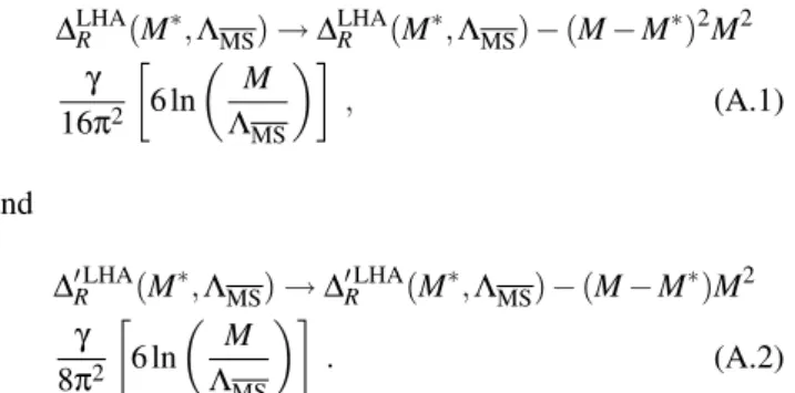
For completeness, let us check numerically the effects of leaving a leading log dependence also in the two point Green’s function with zero external momentum,Γ(2), given
by Eq. (16). Then, ∆LHAR (M∗,ΛMS)→∆
LHA
R (M∗,ΛMS)−(M−M∗) 2M2 γ
16π2
6 ln
M ΛMS
, (A.1)
and
∆′RLHA(M∗,ΛMS)→∆′ LHA
R (M∗,ΛMS)−(M−M∗)M 2
γ 8π2
6 ln
M ΛMS
. (A.2)
In this case, the effective potential gives a first (momentum independent) correction to the effective scalar mass in the vacuum,m∗s,vac. Then, for each energy scale, apart from the BErequirement one also has to fix the parameter set so that the effective scalar meson mass ism∗s,vac=512 MeV. This ef-fective mass is obtained by considering one loop momentum independent self energy
(m∗s,vac)2=m2 s−M2g2s
γ 8π2
6 ln
M
ΛMS
, (A.3)
which clearly indicates thatms(as well asgs) must run with
the energy scale. However, this more cumbersome approach has almost no effect in our best results for K and Msat∗ as table III shows indicating the adequacy of the LHA simple prescription previously adopted.
TABLE III: Same as in table I for the case in whichΓ(2)has a non vanishing leading log andm
sruns with the energy scale.
ΛMS/M K(MeV) Msat∗ /M Cv2 Cs2 g2v g2s ms(MeV)
1.000 468.140 0.718 114.740 183.300 79.782 54.497 512.000
0.975 294.260 0.776 84.456 74.106 58.725 22.032 641.594 0.950 235.660 0.809 67.923 46.297 47.229 13.765 671.839 0.920 202.507 0.832 55.411 31.755 38.529 9.441 687.840
[1] J. D. Walecka, Ann. Phys. (N.Y.)83, 491 (1974); B. D. Serot and J.D. Walecka, Adv. Nucl. Phys.16(1986);
[2] P. Ramond, “Field Theory: a Modern Primer” (Westview Press, 2001); D. Bailin and A. Love,“Introduction to Gauge Field Theory Revised Edition”(Taylor and Francis, 1993). [3] C. H. Johnson, D. J. Horen and C. Mahaux, Phys. Rev. C36,
2252 (1987); C. Mahaux and R. Sartor, Nucl. Phys.A475, 247 (1987); Nucl. Phys.A493, 157 (1989).
[5] J. P. Blaizot, D. Gogny and B. Grammiticos, Nucl. Phys. A265, 315 (1976); J. P. Blaizot, Phys. Rep.64, 171 (1980); H. Krivine, J. Treiner and O. Bohigas, Nucl. Phys. A336, 155 (1980); N. K. Glendenning, Phys. Rev. Lett. 57, 1120 (1986); Phys. Rev. C37, 2733 (1988); M. M. Sharma, W. T. A. Borghols, S. Brandenburg, S. Crona, A. van der Woude and M. N. Harakeh, Phys. Rev. C38, 2562 (1988).
[6] S. A. Chin, Phys. Lett.B62, 263 (1976); Ann. Phys. (N.Y.) 108, 301 (1977).
[7] R. J. Furnstahl, R. J. Perry and B. D. Serot, Phys. Rev. C40, 321 (1989); D. A. Wasson and R. J. Perry, Phys. Rev. C42, 2040 (1990).
[8] A Bielajew and B. Serot, Ann. Phys. (N.Y.)156, 215 (1984). [9] D. P. Menezes, M. B. Pinto and G. Krein, Int. J. of Mod. Phys.
E9, 221 (2000).
[10] J. Boguta and A. R. Bodmer, Nucl. Phys.A292, 413 (1977).
[11] E. K. Heide and S. Rudaz, Phys. Lett.B262, 375 (1991). [12] M. Prakash, P. J. Ellis, E. K. Heidi and S. Rudaz, Nucl.Phys
A575, 583 (1994); S. S. Rocha, A. R. Taurines, C. A. Z. Va-concellos, M. B. Pinto, and M. Dillig, Mod. Phys. Lett. A17, 1335 (2002).
[13] P.A. Henning and P. Manakos, Nucl. Phys.A466, 487 (1987). [14] B.L. Friman and P.A. Henning, Phys. Lett.B206, 579 (1988). [15] P.A. Henning, Phys. Rep.253, 235 (1995).
[16] Wang Zisheng, Ma Zhongyu and Zhuo Yizhong, Phys. Rev. C 55, 3159 (1997).
[17] L. Brown,“Quantum Field Theory”(CUP, 1994).
[18] N. K. Glendenning and S.A. Moszkowski, Phys. Rev. Lett.67, 2414 (1991).