Holistic corpus-based dialectology
Dialetologia holística baseada em corpus
Benedikt Szmrecsanyi* Christoph Wolk**
Freiburg Institute for Advanced Studies Freiburg / Germany
ABSTRACT: This paper is concerned with sketching future directions for corpus-based dialectology. We advocate a holistic approach to the study of geographically conditioned linguistic variability, and we present a suitable methodology, ‘corpus-based dialectometry’, in exactly this spirit. Specifically, we argue that in order to live up to the potential of the corpus-based method, practitioners need to (i) abandon their exclusive focus on individual linguistic features in favor of the study of feature aggregates, (ii) draw on computationally advanced multivariate analysis techniques (such as multidimensional scaling, cluster analysis, and principal component analysis), and (iii) aid interpretation of empirical results by marshalling state-of-the-art data visualization techniques. To exemplify this line of analysis, we present a case study which explores joint frequency variability of 57 morphosyntax features in 34 dialects all over Great Britain.
KEYWORDS: corpus-based dialectology; holistic approach; corpus-based dialectometry; feature aggregates; multivariate analysis; visualization techniques.
RESUMO: Este artigo debruça-se sobre o esboço propositivo de futuras direções para a dialetologia baseada em corpus. Defendemos uma abordagem holística para o estudo da variabilidade linguística geograficamente condicionada, e apresentamos uma metodologia adequada para tal – a dialetometria baseada em corpus. Mais especificamente, defendemos que para que se obtenham todos os resultados esperados da metodologia de corpus, pesquisadores devem: (i) abandonar seu foco exclusivo em traços linguísticos individuais em favor do estudo dos agregados de traços, (ii) amparar-se em métodos computacionais avançados de técnicas de análise multivariada (tais como escalagem multidimensional, análise de clusters, e análise de componente principal), e (iii) auxiliar a interpretação de resultados empíricos através da utilização do estado da arte em técnicas de visualização. A fim de exemplificarmos essa linha de análise, apresentamos um estudo de caso que explora a variabilidade da frequência agregada de 57 traços morfossintáticos de 34 dialetos da Grã-Bretanha.
1. Introduction
The customary data sources in traditional dialectology are dialect dictionaries, dialect atlases, and assorted other competence-centered materials. In the past couple of decades, however, more and more dialect corpora have been coming on-line, and corpus-linguistic methodologies have increasingly found their way into the dialectological toolbox (see ANDERWALD; SZMRECSANYI, 2009 for an overview). This is good news, for compared to survey material corpora arguably yield a more realistic and performance-based linguistic signal. Yet, on the empirical-analytical plane corpus-performance-based approaches to dialectology are still a far cry from the rigor and sophistication customary in survey-based dialectology. This is particularly galling since corpora as a data type offer a host of exciting research opportunities not available otherwise. In this paper, we shall argue that corpus-based dialectologists would be well advised to abandon their customary reliance on single-feature studies in favor of holistic, computational approaches that explore joint variability of feature aggregates. In short, we will be advocating a methodology that we have referred to as CORPUS-BASEDDIALECTOMETRY
(CBDM) elsewhere (cf. SZMRECSANYI, 2008; SZMRECSANYI, 2011).
As a case study to explore CBDM’s analytical potential and to highlight the
benefits of holistic analysis, we shall tap the Freiburg Corpus of English Dialects (FRED) (HERNÁNDEZ, 2006; SZMRECSANYI; HERNÁNDEZ, 2007). FRED contains 368 individual texts and spans approximately 2.4 million words
of running text, consisting of samples (mainly transcribed so-called ‘oral history’ material) of naturalistic, dialectal speech from a variety of sources. Most of these samples were recorded between 1970 and 1990; in most cases, a fieldworker interviewed an informant about life, work, etc. in former days. The 431 informants sampled in the corpus are typically elderly people with a working-class background. The interviews were conducted in 156 different locations (that is, villages and towns) in 34 different pre-1974 counties in Great Britain including the Isle of Man and the Hebrides. The level of areal granularity investigated in the present study will be the county level. This leaves us with 34 dialect objects that will be exemplarily subjected to dialectometrical analysis in the subsequent sections.
of ways in which dialectological datasets can be analyzed holistically: cartographic projections to geography (Section 5.1.), network diagrams (Section 5.2.), and correlational quantitative techniques (Section 5.3.). Section 6 utilizes Principal Component Analysis to identify linguistic structure in the dataset. Section 7 offers some concluding remarks.
2. Holistic analysis – why?
AGGREGATEDATAANALYSIS (also known as DATASYNTHESIS) is concerned
not with the distribution of individual features, properties, or measurements, but with the joint analysis of multiple characteristics. Aggregation is a methodical cornerstone in many academic disciplines. Taxonomists, for instance, typically categorize species not on the basis of a single morphological or genetic criterion, but holistically on the basis of many. By contrast, in linguistics and particularly in corpus linguistics, we find a long and strongly entrenched tradition of looking at individual features in isolation, which is partly a legacy of the discipline’s philological origins, and partly a convenience issue. In any event, the one-feature-at-a-time line of analysis – exceptions such as the multidimensional register studies in the spirit of Biber (1988) notwithstanding – has yielded a corpus-based dialectology literature dominated by an abundance of what Nerbonne (2008) has referred to as ‘single-feature-based studies’. We will refrain from citing actual studies here (but see the survey in ANDERWALD; SZMRECSANYI, 2009), though fictitious titles such as ‘Verbal complementation in West Yorkshire English’ or ‘The KIT vowel in Appalachian English’ are entirely realistic. Now, single-feature
studies like this are completely fine, of course, when it is really the features themselves (verbal complementation, the KIT vowel) that are of analytic
interest. The approach, however, is uninformative and, in fact, woefully inadequate when single-feature analysts endeavor to characterize multidimensional objects such as dialects and the relationships between them, along the lines of research questions such as ‘How does (the grammar and/or phonology and/ or … of) Yorkshire English relate to (the grammar and/or phonology and/or … of) Appalachian English?’. In fact, for addressing questions like these the single-feature approach is about as uninformative and inadequate as a car comparison test whose only criterion is, e.g., the number of cup holders installed.
characterization suggested by the previous feature. For example, Yorkshire English may be progressive in regard to verbal complementation, but conservative as far as verbal agreement is concerned. Thus, there is no guarantee that some dialect or variety will exhibit the same distributional behavior in regard to different features. In addition, individual features may have fairly specific quirks to them that are irrelevant to the big picture and which create noise (NERBONNE, 2009). For instance, the KIT vowel in Appalachian English
may very well be a stark outlier in that dialect’s phonology, a possibility that we cannot rule out unless we proceed holistically and also look at other features. In sum, we offer that holistic data analysis is indispensable whenever the analyst’s attention is turned to the forest (‘dialects’), not the trees (‘dialect features’). Data synthesis and aggregation mitigate the problem of feature-specific quirks, irrelevant statistical noise, and the problem of inherently subjective feature selection, and can thus unearth a more robust, objective, and realistic linguistic signal.
3. Corpus-based dialectometry
The shortcomings of non-holistic analysis have been known since at least the 1930s (cf., for example, BLOOMFIELD, 1984 [1933]: chapter 19). Starting in the 1970s, computationally inclined dialectologists have addressed these worries by developing a methodology known as DIALECTOMETRY.
Dialectometry is defined as the branch of geolinguistics concerned with measuring, visualizing, and analyzing aggregate dialect similarities or distances as a function of properties of geographic space (for seminal work, see SÉGUY, 1971; GOEBL, 1982; GOEBL, 1984; NERBONNE; HEERINGA; KLEIWEG, 1999; HEERINGA, 2004; NERBONNE, 2005; GOEBL, 2006; NERBONNE; KLEIWEG, 2007). Dialectometrical inquiry marshals computational approaches to identify “general, seemingly hidden structures from a larger amount of features” (GOEBL; SCHILTZ, 1997, p. 13) and puts a strong emphasis on quantification, cartographic visualization, and exploratory data analysis to infer patterns from feature aggregates.
Orthodox dialectometry relies on digitized dialect atlases as its primary data source. By contrast, the present contribution outlines a variety of dialectometry that we call CORPUS-BASEDDIALECTOMETRY (henceforth: CBDM).
typically inferior to dialect atlases. Having said that, as a data source, corpora have interesting advantages over dialect atlases. First and foremost, the atlas signal is categorical, exhibits a high level of data reduction, and may hence be less accurate than the corpus signal, which can provide graded frequency information. While the exact cognitive status of text frequencies is admittedly still unclear – for example, we do not currently know about the precise extent to which corpus frequencies correlate with psychological entrenchment (ARPPE; GILQUIN; GLYNN; HILPERT; ZESCHEL, 2010) – we do claim that text frequencies match better with the reality of the input perceived by hearers than discrete atlas classifications. Second, we note that the atlas signal is non-naturalistic and, basically, meta-linguistic in nature. It typically relies on elicitation and questionnaires, and is analytically twice removed (via fieldworkers and atlas compilers) from the analyst. By contrast, text corpora – and, by extension, CBDM – provide more direct access to language form and
function, and may thus yield a more realistic and trustworthy picture. Furthermore, corpus material is more easily extensible in two ways. On the one hand, it is easier to supplement corpus databases with additional material; for example, oral history recordings comparable to the ones used in FRED are
easier to come by than informants that are equally comparable to the ones that completed some atlas questionnaire decades ago. On the other hand, the analysis of atlas data is constrained by the design of the questionnaire, allowing only in a limited way for the study of research questions not originally envisaged. The corpus-based analyst, by contrast, is at more liberty to approach new questions, given that the corpus is of sufficient size.
The well-known major intrinsic drawback of the corpus-based method is that it is unable to deal with textually infrequent phenomena (see, e.g., PENKE; ROSENBACH, 2004, p. 489), and data sparsity is a particular concern when the focus is on syntax and lexis; in this case, a questionnaire study may indeed be the more appropriate research design. Nonetheless, one may justifiably wonder if phenomena that are so infrequent that they cannot be described on the basis of a major text corpus should have a place in an aggregate analysis at all.
4. Methodical preliminaries
The first step in CBDM calls for defining the feature catalogue as the
in feature selection, the goal is to base the analysis on as many features as possible. In the case study at hand, we surveyed the dialectological, variationist, and corpus-linguistic literature on morphosyntactic variability in varieties of English for suitable phenomena. This resulted in a list of p = 57 features, which overlaps with but is not identical to recent comparative English morphosyntax surveys (cf. KORTMANN; SZMRECSANYI, 2004; SZMRECSANYI; KORTMANN, 2009) and the battery of morphosyntax features covered in the Survey of English Dialects (for example, ORTON; SANDERSON; WIDDOWSON, 1978). The Appendix lists the features in the catalogue; for a detailed discussion of the selection criteria, the reader is referred to Szmrecsanyi (2011).
Next, the analyst extracts feature frequencies from the corpus according to best corpus linguistic practice. Szmrecsanyi (2010) details the technicalities of the extraction process in terms of our CBDM case study. Once feature
frequencies are extracted, the analyst will normalize text frequencies, and possibly apply a log-transformation to de-emphasize large frequency differentials and to alleviate the effect of frequency outliers. Lastly, an N × p frequency matrix is created in which the N objects (that is, dialects or varieties) are arranged in rows and the p features in columns, such that each cell in the matrix specifies a particular (normalized and log-transformed) feature frequency. Our CBDM case study thus yields a 34 × 57 frequency matrix: 34
British English dialects, each characterized by a vector of 57 (normalized and log-transformed) text frequencies. The matrix yields a Cronbach’s a (cf.
NUNNALLY, 1978) value of .77, a score that indicates acceptable reliability.
5. Analyzing dialect relationships in the aggregate perspective
where p is the number of features, a1 is the frequency of feature 1 in object a, b1 is the frequency of feature 1 in object b, a2 is the frequency of feature 2 in object a, and so on.
The chart in Figure 1 illustrates the aggregation process. In step , we start out with a fictional 3 × 2 frequency matrix, which has 6 cells specifying frequencies of 2 features in 3 dialects. In step we calculate three distances: the distance between dialects a and b (which we commonsensically define as identical to the distance between dialects b and a), the distance between dialects a and c, and the distance between dialects b and c. In step , we enter these distances into a 3 × 3 distance matrix.
Distance matrices can be analyzed in a myriad ways – numerically, cartographically, and diagrammatically. Our cbdm case study’s 34 × 57 frequency matrix yields a 34 × 34 distance matrix which describes 34 × 33/2 = 561 pairwise distances between the dialect objects under study. The mean morphosyntactic distance is 5.41 Euclidean distance points. As for the dataset-internal dispersion around the mean, we are dealing with a standard deviation of 1.11. This is another way of saying that roughly two thirds of the 561 dialect pairings score a distance within 1.11 points of the mean, and that 95% of all pairwise distances do not deviate more than 2.22 points from the mean. The minimum observable distance in the dataset is 2.32 points (this happens to
1
2
be the morphosyntactic distance between the dialects spoken in the county of Somerset and the county of Wiltshire, two neighboring counties located in the Southwest of England). The maximum observable distance in the dataset is 8.14 points, which is the distance between the dialects spoken in the county of Denbighshire in Wales and the county of Kincardineshire in the Scottish Lowlands. The distance matrix comes with a skewness value of -.06, which indicates a very slight negative skew. The kurtosis value is -.37, which is another way of saying that the distribution of distances is a bit flatter than it would be in a perfectly normal distribution.
5.1. Cartography
5.1.1. Beam maps
Beam maps are comparatively straightforward maps that project distance matrices to geography without much statistical ado. They are easy to read because the map type restricts attention to so-called ‘interpoint’ (i.e. neighbor) relationships (GOEBL, 1982, p. 51). In this spirit, we now turn to Map 1, which features a beam map visually depicting interpoint relationships in our 34 × 34 distance matrix. As for the color coding, note that morphosyntactically distant neighbors are connected by cold (blueish) and thin beams; neighbors that are close morphosyntactically are connected by warm (reddish) and heavy beams. Visual inspection of Map 1 suggests four hotbeds of neighborly similarity in Great Britain. These highlight a very crucial dialect division well-known from the literature – the split between dialects spoken (i) in the Southwest of England, (ii) dialects spoken in the Southeast of England, (iii) dialects spoken in the North of England, and (iv) Scots dialects:
• In the Southwest of England, there is a comparatively marked axis of interpoint similarities running from Cornwall via Devon and Somerset all the way to Wiltshire.
• In the Southeast of England, we note a triangle of relatively modest morphosyntactic similarities connecting Kent, London, and Suffolk. • In the Northern Midlands and the North of England, we find a web
of strong interpoint similarities encompassing Nottinghamshire, Lancashire, Westmorland, Yorkshire, and Durham.
• The Central Scottish Lowlands exhibit a bolt of interpoint similarities involving parts of the urbanized ‘Central Belt’.
5.1.2. Continuum maps
Many geolinguists intuitively assume that geographic proximity predicts dialectal similarity (cf. NERBONNE; KLEIWEG, 2007, p. 154). This section utilizes more advanced cartography – specifically, so-called continuum maps (HEERINGA, 2004) – to map the extent to which linguistic distance is directly proportional to geographic distance such that there are “no real boundaries, but only gradual transitions” (BLOOMFIELD, 1984 [1933], p. 341). We set the scene by utilizing customary Voronoi tesselation (VORONOI, 1907) to assign each dialect site on the map a convex polygon such that each point within the polygon is closer to the generating dialect site than to any other dialect site (note that as our CBDM case study
the radius of the Voronoi polygons to approximately 50km in order to do visual justice to the areal coverage of the dialect corpus). The next step is a computational one and subjects the 34 × 34 distance matrix to Multidimensional Scaling (MDS) (KRUSKAL; WISH, 1978; EMBLETON,
1993), an exploratory statistical technique to reduce a higher-dimensional dataset to a lower-dimensional representation which is more amenable to visualization. We thus scale down our high-dimensional distance matrix to a three-dimensional representation, in which each object (i.e. dialect) has a coordinate in three artificial MDS dimensions. These coordinates are then
mapped to the red-green-blue color scheme, giving each of the Voronoi polygons a distinct hue. Interpetationally, smooth color transitions between dialect polygons emphasize the continuum-like nature of the dialect landscape; abrupt color transitions point to the necessity of alternative explanations.
MAP 2. Continuum similarity. Correlation with distances in the original distance matrix:
Consider, now, the continuum map in Map 2. The MDS solution depicted is
a very accurate one, in that the distances in the three artificial MDS dimensions
correlate highly (r = .95) with the distances in the original 34 × 34 distance matrix. In all, the mosaic pattern in the continuum map suggests that the morphosyntactic dialect landscape in Great Britain is in all not exceedingly continuum-like. For sure, there are some fairly nice micro-continua (in, say, the Southwest of England and in the Central and Northern Scottish Lowlands); notice also how nicely dialects spoken in the North of England fade into Southern Scottish Lowlands dialects. But we also observe rather abrupt transitions, for example between the Central Scottish Lowlands and Southern Scottish dialects (Peebleshire and Selkirkshire). In England, the dialects spoken in Middlesex and Warwickshire are outliers. In Wales, it is Denbighshire that does not fit into the picture.
5.1.3. Cluster maps
MAP 3. Hierarchical agglomerative cluster analysis (matrix updating algorithm: Ward’s method). Left: dendrogram. Right: cluster map
The dialect area scenario may be cartographically explored using cluster maps, a map type which projects the outcome of cluster analysis to geography (HEERINGA, 2004; GOEBL, 2007). As with continuum maps, the starting point is a Voronoi tesselation of map space. Subsequently, the N × N distance matrix is subjected to Hierarchical Agglomerative Cluster Analysis (JAIN; MURTY; FLYNN, 1999), a technique designed to group a number of objects (in this study, dialects) into a smaller number of discrete clusters. While there are many different clustering algorithms, we prefer ‘Ward’s Minimum Variance Method’ (WARD, 1963), an algorithm that tends to create small and even-sized clusters.1 Cluster analysis can be used to generate a so-called ‘dendrogram’
1 Observe that simple clustering can be unstable, which is why we utilize a technique
known as ‘clustering with noise’ (NERBONNE; KLEIWEG; MANNI, 2008): The original distance matrix is clustered repeatedly, adding some random amount of noise (c = s/2)
(cf. Map 3), which depicts cophenetic distances between the clustered objects. The optimal number of clusters can be determined by ‘elbowing’, i.e. diagramming the number of clusters against the fusion coefficient and spotting the ‘elbow’ in the resulting graph (ALDENDERFER; BLASHFIELD, 1984, p. 54). Finally, each of the clusters is assigned a distinct color hue and the Voronoi polygons are colorized accordingly. Map 3 projects clusters in our
CBDM dataset to geography. Despite some geographic incoherence, cluster
analysis does detect an areal pattern:
• We find a geographically modestly coherent red cluster comprising most Southern English measuring points (Middlesex being the exception) plus Nottinghamshire in Central England, Suffolk in East Anglia, and Durham in Northern England.
• We also obtain a geographically fairly coherent green group encompassing the majority of measuring points in Northern England (Westmorland, Yorkshire, Lancashire), the Isle of Man, Shropshire and Leicestershire in Central England, and Glamorganshire in Southern Wales.
• Lastly, we are faced with a blue mixed-bag cluster uniting all measuring points in Scotland plus Northumberland in Northern England plus Denbighshire in Northern Wales plus Warwickshire in Central England plus Middlesex in Southern England.
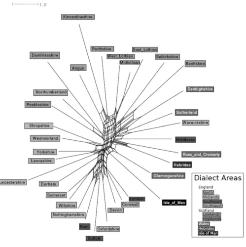
5.2. Network diagrams
2007) purposes, thanks to NeighborNet’s ability to detect conflicting signals and to represent the effects of language contact. The majority of current applications of NeighborNet in linguistics are restricted to the analysis of categorical atlas-type data. In this section we seek to sketch some of the promises the technique holds for frequency-based analyses.
Let us begin by briefly sketching the algorithm that generates the network diagrams. NeighborNet has the same starting point as the previous analyses – a distance matrix.2 As with hierarchical agglomerative cluster analysis,
the distance matrix is searched for the pair of points with the shortest distance. Instead of immediately fusing these points to a single cluster, however, they are just marked, and this procedure is repeated until the same point is marked twice. Then, these points are replaced with two clusters, each representing the doubly marked point in relation to one of its marked neighbors. This process is repeated until only three clusters are left. The fusion sequence can subsequently be used to generate a network-like diagram. This procedure has some beneficial properties. First, the result will not be needlessly complex. For cases where a segment of the data can be adequately represented as a hierarchical tree, the corresponding segment of the network will be tree-shaped. Second, the method will always produce graphs that are planar, i.e. without crossing lines, which aids visual interpretation.
Figure 2 depicts a network based on the FRED 34 × 34 distance matrix;
broad a priori dialect areas are indicated via colored labels. The graph was created using the freely available SplitsTree package (HUSON; BRYANT, 2006). When interpreting such networks, the equivalents of edges connecting two tree nodes in a dendrogram are either individual lines, or sets of parallel lines. In this network, we only find individual lines directly at the leaf nodes, and many sets of parallel lines, combining to the boxy shapes that form the body of the network. Each represents a way of splitting the total set of dialects into exactly two groups. The longer a given line or set of lines, the greater the difference between the groups. To give an example, the comparatively large vertical set of lines directly below the point where Durham joins the network divides the dialects into the following two groups: one group that consists of Nottinghamshire as well as all Southwestern and Southeastern dialects except Middlesex, and another group that contains all other dialects. When two such divisions are not
2 On a technical note, NeighborNet relies on observed distances to create a new
representable as strictly hierarchical, the resulting lines form boxy shapes. Comparing the network to the strict clustering provided by the dendrogram in Map 3, we find that the network shows considerable amounts of incompatible groupings, indicating that a simple hierarchical classification structure does not entirely adequately capture the uncertainty present in the data.
FIGURE 2. Network representation of morphosyntactic distances. Colors indicate a priori dialect areas.
progressing clockwise through Midlands and Northern dialects toward the Scottish dialects at the top. Most of the non-Scottish components of the ‘mixed-bag’ cluster discussed in Section 5.1.3., as well as the Scottish Highlands and the Hebrides, are distributed along the right-hand side. The correspondence between geography and the network is certainly not perfect, as some distinctions – such as the difference between Southeastern and Southwestern English dialects – do not materialize in the graph, and the Midlands are mostly intermingled with either Southern or Northern English dialects. Closer inspection of the individual groupings shows that while some of the large-scale areas, such as the (mostly) Southern group mentioned above, are actually represented by an individual split, others (such as the North of England) are not really a single group, but a collection of smaller ones with interlocking resemblances. As one moves from the center of the network toward the individual dialects, such structure becomes apparent throughout the graph, and it is here where the advantage of networks over tree representations is easiest to see. For example, the sub-tree of the dendrogram in Map 3 that connects the rather central Oxfordshire to Nottinghamshire, Kent and Suffolk is still present in the network. Nonetheless, there is also a new, incompatible grouping of Oxfordshire with Devon to the West. This suggests that individual similarities in both directions exist, beyond those that can be explained by the fact that each is a member of the group of (mostly) Southern English dialects. A similar case can be found in the Scottish Lowlands, where the measuring points East Lothian and Midlothian form a rather treelike subgroup. West Lothian, by contrast, is notably removed toward the northern Lowlands. Again, a geographic interpretation is possible, as West Lothian is closer to the northern areas by land and the fjord that separates them from the Lothians, the Firth of Forth, widens considerably to its east.
5.3. Quantifying the effect of language-external predictors
CBDM is intrinsically quantitative, yet it is fair to say that the foregoing
discussion has relied heavily on interpreting cartographic projections to geography and other diagrammatic representations. However, the analyst may also correlate language-external parameters with linguistic distances to precisely quantify the extent to which dialect distances are predictable from language-external factors in the aggregate perspective. Starting out with an N × N linguistic distance matrix, the name of the game is creating parallel language-external distance matrices, one for each predictor to be tested. In the simplest case, each of these language-external distance matrices is then correlated with the linguistic distance matrix by calculating, e.g., a Pearson product-moment correlation coefficient. The language-external predictor that scores the highest coefficient is the best predictor of linguistic distances (more sophisticated research designs may marshal regression analysis or similar techniques).
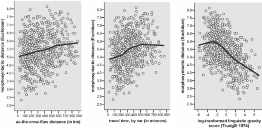
To exemplify, let us revisit our dataset on dialect variability in Great Britain. We will correlate the 34 × 34 morphosyntactic distance matrix with three language external distance matrices:
• As-the-crow-flies distances. Using a trigonometry formula on the FRED
county coordinates, it is computationally trivial to calculate pair wise as-the-crow-flies distances. A proxy for the likelihood of social contact, as-the-crow-flies distance is the most popular geographic distance measure in the dialectometry literature (for example, GOEBL, 2001; GOOSKENS; HEERINGA, 2004; SHACKLETON, 2007). • Least-cost travel times. Speakers do not actually have wings, so we may
presume that what really matters for dialect distances is how much time it would take a human traveler to get from point A to point B (GOOSKENS, 2005; SZMRECSANYI to appear). To calculate this measure, we turned to Google Maps (<http://maps.google.co.uk/>), which has a route finder tool that allows the user to enter longitude/latitude pairings for two locations to obtain a least-cost travel route and, crucially, an estimate of the total travel time. We queried Google Maps for all 34 × 33/2 = 561 dialect pairings in our dataset, thus obtaining pair wise least-cost-travel time estimates.3
3 We fully acknowledge that matching linguistic data sourced from speakers born
• Linguistic gravity indices. Trudgill (1974) suggested a Newtonian gravity model to account for geographic diffusion of linguistic features, conjecturing that “the interaction (M) of a centre i and a centre j can be expressed as the population of i multiplied by the population of j divided by the square of the distance between them” (1974, p. 233). Using this formula, we calculated log-transformed (to mitigate the effect of population outliers) linguistic gravity values for each of the 561 data pairings in our database, feeding in least-cost travel time as geographic distance measure and early twentieth century population figures4 (in thousands) as a proxy for speaker community size.
Nonetheless, we submit that the procedure is not fatally flawed, as modern infrastructure can be argued to actually follow, to a large extent, historical travel routes, trade patterns, and avenues of social contact.
4 Specifically, we used 1901 population figures, as published in the Census of England
and Wales, 1921 and the Census of Scotland, 1921. These documents are available online at <http://histpop.org/>.
FIGURE 3. Correlating distance matrices: morphosyntactic distances versus (i) as-the-crow-flies distance (left) (r = .21, p < .001, R2=4.4%), (ii) least-cost travel time (middle) (r = .27, p < .001, R2=7.4%), and (iii) log-transformed linguistic gravity indices (right) (r = -.49, p < .001, R2=24.1%). Each dot represents one unique dialect pairing. Solid lines are LOESS
Figure 3 provides three scatterplots that graph morphosyntactic distances against the language-external distance measures listed above. The direction of the effect is the theoretically expected one throughout. Increasing as-the-crow-flies distance and increasing least-cost travel time predict increasing morphosyntactic distance; conversely, increasing linguistic gravity indices predict decreasing morphosyntactic distance. The R2 values suggest that as-the-crow flies distance accounts for a meager 4.4% of the morphosyntactic variance, least-cost travel time for 7.4%, and linguistic gravity – and this is a share that one can start writing home about – for 24.1%. Hence, by factoring in speaker community size in addition to geographic distance, we can explain up to a quarter of the aggregate variance in morphosyntactic dialect distances. This does not mean, of course, that cartographic projections to geography – which, after all, inherently draw on as-the-crow-flies distances – are somehow ‘wrong’; but we do have an explanation here why, say, the cluster map in Map 3 is not maximally homogeneous geographically.
6. Towards identifying linguistic structure
By virtue of analyzing distance matrices which are derived from feature frequencies but which, once the derivation is complete, are completely agnostic of frequencies, the analyses presented in the previous sections were uncompromisingly holistic. However, it is possible to link aggregate patterns of variability to the distribution of individual features, and in so doing detect linguistic structure in aggregate comparison (cf. NERBONNE, 2006). To showcase this approach, we will now utilize Principal Component Analysis (PCA)
for the sake of addressing two questions: First – on the linguistic/structural level – to what extent do high text frequencies of some feature predict high or low text frequencies of other features? Second – on the geographical plane – how do features thus gang up to create areal patterns?
PCA is a multivariate dimension-reduction technique that transforms a
set of high-dimensional vectors (in our case, 57-dimensional feature frequency vectors) into a set of lower-dimensional vectors (so-called ‘principal components’, which we will interpret as feature bundles) that preserve as much information in the original dataset as possible (DUNTEMAN, 1989, p. 7).
PCA is a fairly popular exploratory analysis method; in linguistics, PCA and
related techniques are customary in multidimensional studies of register variation (cf. BIBER, 1988). In dialectology, PCA (and a close cousin, factor
NERBONNE, 2006; WIELING; HEERINGA; NERBONNE, 2007; LEINONEN, 2008). We started out by subjecting the 34 × 57 frequency matrix specifying 57 normalized and log-transformed feature frequencies for each of the 34 FRED dialects (cf. Section 4) to PCA.5 As output, PCA generates
two sets of statistics: component loadings, which measure the importance of individual linguistic features in particular principal components; and component scores, which measure the strength of particular components in particular dialect objects as a function of each feature’s frequency value in that dialect object and the feature’s component loading in a given component.
PCA extracted 15 components from our case study dataset, of which we
will discuss the first three – accounting collectively for about 37% of the morphosyntactic variance – in some detail. The first principal component (PC1), which captures the main dimension of variation, accounts for 17.2%
of the variance in the dataset. Adopting a common practice in PCA
interpretation (DUNTEMAN, 1989, p. 51), we will select one feature with a particularly high loading to label the principal component in question. The feature loading highest on PC1 is feature [33] (multiple negation, as in don’t you make no damn mistake [FREDCON005]), with a component loading of .85.
This is why we consider PC1 the ‘multiple negation component’. The
component is associated with a variety of other broad dialect features loading highly on PC1, such as the negator ain’t (feature [32], as in people ain’t got no money [FREDNTT013]), don’t with 3rd person singular subjects (feature [40],
as in this man don’t come up to it [FREDSOM032]), and as what or than what in comparative clauses (feature [49], as in we done no more than what other
5 We would like to emphasize that like most statistical analysis techniques, PCA does
5
8
2
RBLA
, Belo Horizonte, v
. 11, n. 2, p. 561-592, 2011
kids used to do [FREDLEI002]). The leftmost projection in Map 4 projects
component scores of PC1 to geography. The projection makes amply clear that
the multiple negation component has, despite some outliers (Warwickshire, Middlesex) a very nice South-North distribution: the component is very characteristic of dialects in the South of Great Britain, and becomes increasingly less important as one moves North. In fact, component scores exhibit over 40% of shared variance (r = .64, p < .001) with geographic latitude scores.
PC2 seeks to explain as best as it can the variation left over in the dataset
after the variance explained by PC1 is taken out of the picture, and in this
endeavor it manages to capture 11.1% of the variance. Features loading high on PC2 are typically features that are close to the standard and which would
have non-standard alternatives, which we typically also check in the feature catalogue. Consider feature [11] (cardinal number + years, as in ten years later [FREDHEB006]) – in many dialects, one would hear ten year later, which we investigate via feature [12]. Feature [11] is a strong loader on PC2 (.71), and
so is feature [46] (wh-relativization, as in the man who has the boat [FRED HEB028]) and feature [2] (standard reflexives, as in they was all for theirselves [FRED NTT002]). We thus choose to label PC2 the ‘wh-relativization component’. Areally, PC2 has not nearly as nice a geographical distribution as PC1, exhibiting as it does a mosaic pattern (cf. the middle projection in Map
4). It is clear, though, that those dialects in which the wh-relativization component is particularly popular include all of the comparatively ‘young’ dialects in Northern Wales (Denbighshire) and the Scottish Highlands (the Hebrides, Ross and Cromarty, and Sutherland). These, in other words, are dialects that are especially close to Standard English.
PC3 accounts for 8.9% of the left-over variance. We dub PC3 the ‘-nae component’, as the negative suffix –nae (feature [31], as in I cannae mind of that [FREDNBL003]) loads high on the component (.59), as does archaic ye (feature [4], as in ye’d dancing every week [FREDANS001]). The connoisseur will
notice immediately that these are stereotypical Scots features – and indeed, the rightmost projection in Map 4 (which projects PC3 component scores to
geography) highlights the -nae component’s popularity in the Scottish Lowlands. In fact, the component creates a North-South distribution such that geographic latitude scores overlap with PC3 component scores to 13%
7. Conclusions and future directions
This paper has advocated an approach – CORPUS-BASEDDIALECTOMETRY
(CBDM) in short – to the study of geographically conditioned linguistic
variability that holistically focuses on the wood and not on the trees. In this spirit, we have argued that corpus-based dialectologists
• would be well-advised to abandon their exclusive focus on individual linguistic features in favor of the study of feature aggregates;
• should reap analytical benefits from utilizing computationally advanced6 multivariate analysis techniques (multidimensional scaling,
cluster analysis, principal component analysis);
• ought to aid interpretation of their results by drawing on various advanced visualization techniques (cartographic projections to geography, network diagrams, and so on).
In this spirit, we hope to have demonstrated that the study of many features in many dialects, coupled with advanced computational analysis methods and sophisticated visualization techniques, can yield insights and generalizations that must remain elusive to the analyst who is beholden to the philologically inspired study of a particular feature in maybe a couple of dialects. For example, our case study on British English dialects has indicated, among other things, that aggregate morphosyntactic variability in Great Britain is, on the whole, not consistently organized along the lines of a dialect continuum, and that we are dealing with some fairly cohesive dialect areas. The layered perspective afforded by principal component analysis subsequently identified those linguistic features that have a continuous geographic distribution (such as features associated with the ‘multiple negation component’), and those that don’t. We think it is fair to say that the breadth of these statements would be hard to come by in any single-feature study, no matter how interesting the feature.
The methodology sketched in this contribution is, of course, not limited to morphosyntactic phenomena. Phonology, lexis, and even pragmatics are all in principle amenable to dialectometrical analysis using a
6 By ‘computationally advanced’ we mean analysis techniques that – unlike e.g.
corpus-based approach. There is even the intriguing possibility of aggregating not ‘surfacy’ feature frequencies but ‘deep’ feature conditionings (e.g. via probabilistic regression weights), a feat that is simply not possible on the basis of decontextualized survey data. Basing future extensions to the CBDM tool set
on a probabilistic basis would furthermore allow taking variation on the level of the speaker into account, concerning both how the independent effects of other factors such as gender and speaker age influence language variation and how homogeneous individual counties really are. Also note that CBDM can be
applied to any corpus in which we find geographic variability. This includes not only dialect corpora in the traditional sense, but also corpora sampling geographically non-contiguous regional language varieties (such as the International Corpus of English) or corpora concerned with variation in written, not spoken, language (such as the letters-to-the-editor corpus analyzed in Grieve 2009).
References
ALDENDERFER, M. S.; BLASHFIELD, R. K. Cluster Analysis. Newbury Park,
London, New Delhi: Sage Publications, 1984.
ANDERWALD, L.; SZMRECSANYI, B. Corpus linguistics and dialectology.
In: LÜDELING, A.; KYTÖ, M. (Ed.). Corpus Linguistics. An International
Handbook. Handbücher zur Sprache und Kommunikationswissenschaft/ Handbooks of Linguistics and Communication Science. Berlin / New York: Mouton de Gruyter, 2009.
ARPPE, A.; GILQUIN, G.; GLYNN, D.; HILPERT, M.; ZESCHEL, A. Cognitive Corpus Linguistics: Five points of debate on current theory and methodology. Corpora, v. 5, n. 2, p. 1-27, 2010.
BIBER, D. Variation across Speech and Writing. Cambridge: Cambridge
University Press, 1988.
BLOOMFIELD, L. Language. Chicago: University of Chicago Press, 1984
[1933].
BRYANT, D.; MOULTON, V. Neighbor-Net: An Agglomerative Method for the Construction of Phylogenetic Networks. Mol. Biol. Evol., v. 21, n. 2, p. 255-265, 2004.
CYSOUW, M. New approaches to cluster analysis of typological indices. In:
KÖHLER, R.; GRZBEK, P. (Ed.). Exact Methods in the Study of Language and
DRESS, A. W. M.; HUSON, D. H. Constructing Splits Graphs. IEEE/ACM Transactions on Computational Biology and Bioinformatics (TCBB), v. 1, n. 3, p. 109-115, 2004.
DUNTEMAN, G. H. Principal components analysis. Newbury Park: Sage
Publications, 1989.
EMBLETON, S. Multidimensional scaling as a dialectometrical technique:
Outline of a research project. In: KÖHLER, R.; RIEGER, B. (Ed.). Contributions
to quantitative linguistics. Dordrecht: Kluwer, 1993.
GOEBL, H. Dialektometrie: Prinzipien und Methoden des Einsatzes der
Numerischen Taxonomie im Bereich der Dialektgeographie. Wien: Österreichische Akademie der Wissenschaften, 1982.
GOEBL, H. Dialektometrische Studien: Anhand italoromanischer, rätroromanischer und galloromanischer Sprachmaterialien aus AIS und ALF. Tübingen: Niemeyer, 1984. 3 v.
GOEBL, H. Arealtypologie und Dialektologie. In: HASPELMATH, M.; E.
KÖNIG, E.; OESTERREICHER, W.; RAIBLE, W. (Ed.). Language Typology
and Language Universals / La typologie des langues et les universaux linguistiques / Sprachtypologie und sprachliche Universalien: An International Handbook / Manuel international / Ein internationales Handbuch. Berlin, New York: Walter de Gruyter, 2001. v. 2.
GOEBL, H. Recent Advances in Salzburg Dialectometry. Literary and Linguistic
Computing, v. 21, n. 4, p. 411-435, 2006.
GOEBL, H. A bunch of dialectometric flowers: a brief introduction to dialectometry. In: SMIT, U.; DOLLINGER, S.; HÜTTNER, J.; KALTENBÖCK,
G.; LUTZKY, U. (Ed.). Tracing English through time: Explorations in language
variation. Wien: Braumüller, 2007.
GOEBL, H.; SCHILTZ, G. A dialectometrical compilation of CLAE 1 and CLAE 2: Isoglosses and dialect integration. In: VIERECK, W.; RAMISCH, H.
(Ed.). Computer developed linguistic atlas of England (CLAE). Tübingen: Max
Niemeyer Verlag, 1997. v. 2.
GOOSKENS, C. Traveling time as a predictor of linguistic distance.
Dialectologia et Geolinguistica, v. 13, p. 38-62, 2005.
GOOSKENS, C.; HEERINGA, W. Perceptive evaluation of Levenshtein dialect
distance measurements using Norwegian dialect data. Language Variation and
GRIEVE, J. A Corpus-Based Regional Dialect Survey of Grammatical Variation in Written Standard American English. 340f. 2009. PhD (Dissertation) – Northern Arizona University.
HAIMERL, E. Database Design and Technical Solutions for the Management,
Calculation, and Visualization of Dialect Mass Data. Literary and Linguistic
Computing, v. 21, n. 4, p. 437-444, 2006.
HEERINGA, W. Measuring dialect pronunciation differences using Levenshtein
distance, 2004. 312f. PhD (Dissertation) – University of Groningen.
HEERINGA, W.; NERBONNE, J. Dialect areas and dialect continua. Language
Variation and Change, v. 13, n. 3, p. 375-400, 2001.
HERNÁNDEZ, N. User’s Guide to FRED. URN:
urn:nbn:de:bsz:25-opus-24895, URL: http://www.freidok.uni-freiburg.de/volltexte/2489/. Freiburg: University of Freiburg, 2006.
HUSON, D. H.; BRYANT, D. Application of phylogenetic networks in evolutionary studies. Molecular Biology Evolution, v. 23, n. 2, p. 254-267, 2006.
JAIN, A. K.; MURTY, M. N.; FLYNN, P. J. Data clustering: a review. ACM
Computing Surveys, v. 31, n. 3, p. 264-323, 1999.
KORTMANN, B.; SZMRECSANYI, B. Global synopsis: morphological and syntactic variation in English. In: KORTMANN, B.; SCHNEIDER, E.;
BURRIDGE, K.; MESTHRIE, R.; UPTON, C. (Ed.). A Handbook of Varieties
of English. Berlin/New York: Mouton de Gruyter, 2004. v. 2.
KRUSKAL, J. B.; WISH, M. Multidimensional Scaling. Newbury Park, London /
New Delhi: Sage Publications, 1978.
LEINONEN, T. Factor Analysis of Vowel Pronunciation in Swedish Dialects.
International Journal of Humanities and Arts Computing, v. 2, n. 1-2, p. 189-204, 2008. MCMAHON, A.; HEGGARTY, P.; MCMAHON, R.; MAGUIRE, W. The sound patterns of Englishes: representing phonetic similarity. English Language and Linguistics, v. 11, n. 1, p. 113-142, 2007.
MCMAHON, A. M. S.; MCMAHON, R. Language classification by numbers.
Oxford New York: Oxford University Press, 2005.
NERBONNE, J. Computational Contributions to Humanities. Linguistic and
Literary Computing, v. 20, n. 1, p. 25-40, 2005.
NERBONNE, J. Identifying Linguistic Structure in Aggregate Comparison.
NERBONNE, J. Variation in the aggregate: an alternative perspective for variationist linguistics. In: DEKKER, K.; MACDONALD, A.; NIEBAUM, H.
(Eds.); Northern Voices: Essays on Old Germanic and Related Topics offered to
Professor Tette Hofstra. Leuven: Peeters, 2008.
NERBONNE, J. Data-driven dialectology. Language and Linguistics Compass,
v. 3, n. 1, p. 175-198, 2009.
NERBONNE, J.; HEERINGA, W.; KLEIWEG, P. Edit Distance and Dialect
Proximity. In: SANKOFF, D.; KRUSKAL, J. (Ed.). Time Warps, String Edits and
Macromolecules: The Theory and Practice of Sequence Comparison. Stanford: CSLI Press, 1999.
NERBONNE, J.; KLEIWEG, P. Toward a Dialectological Yardstick. Journal of
Quantitative Linguistics, v. 14, n. 2, p. 148-166, 2007.
NERBONNE, J.; KLEIWEG, P.; MANNI, F. Projecting dialect differences to geography: bootstrapping clustering vs. clustering with noise. In: PREISACH,
C.; SCHMIDT-THIEME, L.; BURKHARDT, H.; DECKER, R. (Ed.). Data
Analysis, Machine Learning, and Applications. Proceedings of the 31st Annual Meeting of the German Classification Society. Berlin: Springer, 2008.
NUNNALLY, J. C. Psychometric Theory. McGraw-Hill, 1978.
ORTON, H.; SANDERSON, S.; WIDDOWSON, J. D. A. The Linguistic Atlas
of England. London, Atlantic Highlands, N.J.: Croom Helm, 1978.
PENKE, M.; ROSENBACH, A. What counts as evidence in linguistics? An introduction. Studies in Language, v. 28, n. 3, p. 480-526, 2004.
SÉGUY, J. La relation entre la distance spatiale et la distance lexicale. Revue de Linguistique Romane, v. 35, p. 335-357, 1971.
SHACKLETON, R. G. J. English-American Speech Relationships: A Quantitative Approach. Journal of English Linguistics, v. 33, n. 2, p. 99-160, 2005.
SHACKLETON, R. G. J. Phonetic variation in the traditional English dialects: a computational analysis. Journal of English Linguistics, v. 35, n. 1, p. 30-102, 2007.
SZMRECSANYI, B. Corpus-based dialectometry: aggregate morphosyntactic variability in British English dialects. International Journal of Humanities and Arts Computing, v. 2, n. 1-2, p. 279-296, 2008.
SZMRECSANYI, B. The morphosyntax of BrE dialects in a corpus-based
SZMRECSANYI, B. Corpus-based dialectometry – a methodological sketch.
Corpora, v. 6, n. 1, 2011.
SZMRECSANYI, B. Geography is overrated. In: HANSEN, S.; SCHWARZ,
C.; STOECKLE, P.; STRECK, T. (Ed.). Dialectological and folk dialectological
concepts of space. Berlin, New York: Walter de Gruyter, to appear.
SZMRECSANYI, B.; HERNÁNDEZ, N. Manual of Information to accompany
the Freiburg Corpus of English Dialects Sampler (“FRED-S”). URN: urn:nbn:de:bsz:25-opus-28598, URL: http://www.freidok.uni-freiburg.de/ volltexte/2859/. Freiburg: University of Freiburg, 2007.
SZMRECSANYI, B.; KORTMANN, B. The morphosyntax of varieties of English worldwide: a quantitative perspective. Lingua, v. 119, n. 11, p. 1643-1663, 2009. TRUDGILL, P. Linguistic change and diffusion: description and explanation in sociolinguistic dialect geography. Language in Society, v. 2, p. 215-246, 1974. VIERECK, W. Linguistic atlases and dialectometry: The survey of English dialects. In: KIRK, J. M.; SANDERSON, S.; WIDDOWSON, J. D. A. (Ed.).
Studies in linguistic geography: The dialects of English in Britain and Ireland. London: Croom Helm, 1985.
VORONOI, G. Nouvelles applications des paramètres continus à la théorie des
formes quadratiques. Journal für die Reine und Angewandte Mathematik, v. 133,
p. 97-178, 1907.
WARD, J. H. J. Hierarchical grouping to optimize an objective function. Journal of the American Statistical Association, v. 58, p. 236-244, 1963.
WIELING, M.; HEERINGA, W.; NERBONNE, J. An aggregate analysis of
pronunciation in the Goeman-Taeldeman-van Reenen-Project data. Taal en
Appendix: the feature catalogue
NOTE: see Szmrecsanyi (2010) for a version of the feature catalogue annotated
with linguistic examples
A. Pronouns and determiners [1] non-standard reflexives [2] standard reflexives [3] archaic thee/thou/thy [4] archaic ye
[5] us [6] them
B. The noun phrase
[7] synthetic adjective comparison [8] the of-genitive
[9] the s-genitive
[10] preposition stranding [11] cardinal number + years [12] cardinal number + year-Ø
C. Primary verbs
[13] the primary verb TODO
[14] the primary verb TOBE
[15] the primary verb TOHAVE
[16] marking of possession – HAVEGOT
D. Tense and aspect
[17] the future marker BEGOINGTO
[18] the future markers WILL/SHALL
[19] WOULD as marker of habitual past
[20] used to as marker of habitual past [21] progressive verb forms
[22] the present perfect with auxiliary BE
E. Modality
[24] marking of epistemic and deontic modality: MUST
[25] marking of epistemic and deontic modality: HAVETO
[26] marking of epistemic and deontic modality: GOTTO
F. Verb morphology
[27] a-prefixing on -ing-forms
[28] non-standard weak past tense and past participle forms [29] non-standard past tense done
[30] non-standard past tense come
G. Negation
[31] the negative suffix -nae [32] the negator ain’t [33] multiple negation [34] negative contraction [35] auxiliary contraction [36] never as past tense negator [37] WASN’T
[38] WEREN’T
H. Agreement
[39] non-standard verbal -s
[40] don’t with 3rd person singular subjects
[41] standard doesn’t with 3rd person singular subjects
[42] existential/presentational there is/was with plural subjects [43] absence of auxiliary BE in progressive constructions
[44] non-standard WAS
[45] non-standard WERE
I. Relativization
Recebido em 31/08/2010. Aprovado em 08/05/2011.
J. Complementation
[49] as what or than what in comparative clauses [50] unsplit for to
[51] infinitival complementation after BEGIN, START, CONTINUE, HATE,
and LOVE
[52] gerundial complementation after BEGIN, START, CONTINUE, HATE,
and LOVE
[53] zero complementation after THINK, SAY, and KNOW
[54] that complementation after THINK, SAY, and KNOW
K. Word order and discourse phenomena
[55] lack of inversion and/or of auxiliaries in wh-questions and in main clause yes/no-questions
[56] the prepositional dative after the verb GIVE