ACPD
11, 6259–6299, 2011Temperature dependent response
of ozone to NOx
B. W. LaFranchi et al.
Title Page
Abstract Introduction
Conclusions References
Tables Figures
◭ ◮
◭ ◮
Back Close
Full Screen / Esc
Printer-friendly Version Interactive Discussion
Discussion
P
a
per
|
Dis
cussion
P
a
per
|
Discussion
P
a
per
|
Discussio
n
P
a
per
|
Atmos. Chem. Phys. Discuss., 11, 6259–6299, 2011 www.atmos-chem-phys-discuss.net/11/6259/2011/ doi:10.5194/acpd-11-6259-2011
© Author(s) 2011. CC Attribution 3.0 License.
Atmospheric Chemistry and Physics Discussions
This discussion paper is/has been under review for the journal Atmospheric Chemistry and Physics (ACP). Please refer to the corresponding final paper in ACP if available.
Observations of the temperature
dependent response of ozone to NO
x
reductions in the Sacramento, CA urban
plume
B. W. LaFranchi1,*, A. H. Goldstein2,3, and R. C. Cohen1,4
1
Department of Chemistry, University of California, Berkeley, CA, USA 2
Department of Environmental Science, Policy, and Management, University of California, Berkeley, CA, USA
3
Department of Civil and Environmental Engineering, University of California, Berkeley, USA 4
Department of Earth and Planetary Science, University of California, Berkeley, USA *
now at: Center for Accelerator Mass Spectrometry, Lawrence Livermore National Laboratory, Livermore, CA, USA
Received: 12 January 2011 – Accepted: 7 February 2011 – Published: 22 February 2011
Correspondence to: R. C. Cohen ([email protected])
ACPD
11, 6259–6299, 2011Temperature dependent response
of ozone to NOx
B. W. LaFranchi et al.
Title Page
Abstract Introduction
Conclusions References
Tables Figures
◭ ◮
◭ ◮
Back Close
Full Screen / Esc
Printer-friendly Version Interactive Discussion
Discussion
P
a
per
|
Dis
cussion
P
a
per
|
Discussion
P
a
per
|
Discussio
n
P
a
per
|
Abstract
Observations of NOx in the Sacramento, CA region show that mixing ratios decreased by 30% between 2001 and 2008. Here we use an observation-based method to quan-tify net ozone production rates in the outflow from the Sacramento metropolitan region and examine the O3 decrease resulting from reductions in NOx emissions. This
ob-5
servational method does not rely on assumptions about detailed chemistry of ozone production, rather it is an independent means to verify and test these assumptions. We use an instantaneous steady-state model as well as a detailed 1-D plume model to aid in interpretation of the ozone production inferred from observations. In agreement with the models, the observations show that early in the plume, the NOx dependence
10
for Ox (Ox=O3+NO2) production is strongly coupled with temperature, suggesting that temperature-dependent biogenic VOC emissions can drive Oxproduction between NOx-limited and NOx-suppressed regimes. As a result, NOxreductions were found to be most effective at higher temperatures over the 7 year period. We show that viola-tions of the California 1-hour O3standard (90 ppb) in the region have been decreasing
15
linearly with decreases in NOx (at a given temperature) and predict that reductions of NOxconcentrations (and presumably emissions) by an additional 30% (relative to 2007 levels) will eliminate violations of the state 1 h standard in the region. If current trends continue, a 30% decrease in NOx is expected by 2012, and an end to violations of the 1 h standard in the Sacramento region appears to be imminent.
20
1 Introduction
Many populated regions worldwide have chronically high levels of summertime ozone produced during the photochemical oxidation of carbon monoxide (CO) and volatile organic compounds (VOCs) in the presence of NOx (NOx=NO+NO2). Protecting human health (Uysal and Schapira, 2003; Trasande and Thurston, 2005; McClellan
25
ACPD
11, 6259–6299, 2011Temperature dependent response
of ozone to NOx
B. W. LaFranchi et al.
Title Page
Abstract Introduction
Conclusions References
Tables Figures
◭ ◮
◭ ◮
Back Close
Full Screen / Esc
Printer-friendly Version Interactive Discussion
Discussion
P
a
per
|
Dis
cussion
P
a
per
|
Discussion
P
a
per
|
Discussio
n
P
a
per
|
2005; Feng and Kobayashi, 2009; Fuhrer, 2009) has required local regulation aimed at reducing VOC and NOxlevels.
Two informative examples of this are Mexico City (Zavala et al., 2009) and Beijing (Tang et al., 2009), which have been subject to two contrasting emission control strate-gies. In Mexico City, VOC emissions decreased significantly between 1992 and 2006
5
while NOx emissions stayed relatively constant; O3 concentrations decreased during this time at a rate close to 3 ppb year−1. In contrast, in Beijing, O3 concentrations in-creased over a 5 year period, from 2001 to 2006, in response to controls on NOxwith no corresponding reduction in VOC emissions. The results observed in both cities are in line with what would be predicted, in a qualitative sense, from the chemical
mecha-10
nisms of O3production in a VOC-limited atmosphere, typical of polluted cities.
The contrasting examples of Mexico City and Beijing show that the way in which emission controls are implemented can result in varying levels of success, or in some cases, detriment, in controlling O3 concentrations. Complicating matters, however, is that the O3response to identical control strategies is not always the same in different
15
regions. For example, in Los Angeles, combined VOC and NOx controls resulted in a nearly 50% decrease in peak 1 h O3 concentrations from 1990 (310 ppb) to 2007 (159 ppb), however the San Joaquin Valley in Central California, which was subject to essentially the same controls, showed only a marginal decrease in peak 1 h O3 (164 ppb to 142 ppb) over this time frame (Cox et al., 2009).
20
While we have an adequate qualitative understanding of the response of O3 to NOx and/or VOC reductions, a quantitative analysis remains elusive (e.g. Thornton et al., 2002), presumably because of our incomplete knowledge of the relevant emissions and photochemistry and our inability to represent the meteorology with sufficient accuracy. As it is unclear which aspects of our chemical understanding need improvement, direct
25
tests of the mechanisms by comparison to observations in the ambient atmosphere are needed.
ACPD
11, 6259–6299, 2011Temperature dependent response
of ozone to NOx
B. W. LaFranchi et al.
Title Page
Abstract Introduction
Conclusions References
Tables Figures
◭ ◮
◭ ◮
Back Close
Full Screen / Esc
Printer-friendly Version Interactive Discussion
Discussion
P
a
per
|
Dis
cussion
P
a
per
|
Discussion
P
a
per
|
Discussio
n
P
a
per
|
realized in the atmosphere. Day-of-week effects on ozone are a close approximation to a control experiment, because NOx emissions typically decrease significantly on weekends with relatively small changes in VOC emissions. Still, in most locations, meteorology varies too much to directly compare weekends and weekdays in a given year, and long term decreases in NOx and VOCs, along with changes in land use,
5
makes year to year comparisons subject to the difficulties of interpreting an experiment where many things have changed at once.
The Sacramento, California (38.58◦N, 121.49◦W) urban plume o
ffers a rare oppor-tunity for evaluating effects of changes in a single parameter, NOx concentrations, on atmospheric chemistry using ambient measurements. The local topography in the
re-10
gion results in an extremely stable wind field, with upslope flow during the daytime, and downslope flow at night, driven by heating and cooling in California’s central valley (e.g. Carroll and Dixon, 2002; Dillon et al., 2002). The VOCs that control ozone pro-duction in the region are predominantly biogenic (Dreyfus et al., 2002; Cleary et al., 2005; Steiner et al., 2008). Variability in NOx, therefore, is completely decoupled from
15
variability in VOCs in the region.
NOx mixing ratios in the Greater Sacramento Area (as we will discuss below) and throughout Northern California (Ban-Weiss et al., 2008; Cox et al., 2009; Russell et al., 2010) have been in steady decline for over a decade, thus facilitating an atmospheric experiment in which only a single variable in the ozone production system has been
20
changed (at a given temperature). Previous work has investigated the effect of day-of-week changes in NOxemissions on O3production in the region. Here, with variability in NOx occurring on both day-of-week and interannual time-scales, we are able to compare the effects of NOx reductions within a single year (weekdays vs. weekends) to the equivalent NOx reductions on weekdays several years later.
25
ACPD
11, 6259–6299, 2011Temperature dependent response
of ozone to NOx
B. W. LaFranchi et al.
Title Page
Abstract Introduction
Conclusions References
Tables Figures
◭ ◮
◭ ◮
Back Close
Full Screen / Esc
Printer-friendly Version Interactive Discussion
Discussion
P
a
per
|
Dis
cussion
P
a
per
|
Discussion
P
a
per
|
Discussio
n
P
a
per
|
(Sect. 4). We will compare our observations to results from a steady-state model and a time-dependent Lagrangian plume model (Sect. 5) and discuss the implications of our results for air quality in the region (Sect. 6).
2 The sacramento urban plume
Due to its extremely regular, topographically-driven wind patterns, the Sacramento
re-5
gion can be represented as a simple flow reactor with dilution (Carroll and Dixon, 2002; Dillon et al., 2002; Perez et al., 2009). This Lagrangian representation holds for a significant portion of the year and greatly facilitates the understanding of changes in photochemical conditions over diurnal (Murphy et al., 2006a; Day et al., 2009), weekly (Murphy et al., 2007), seasonal (Murphy et al., 2006a; Day et al., 2008; Farmer and
10
Cohen, 2008), and, as in the present study, inter-annual timescales.
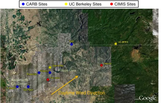
A map of the Greater Sacramento Area (GSA) and the downwind regions influenced by the urban plume is shown in Fig. 1. We will refer to three different sub-regions in this discussion: the urban core, the suburbs, and the foothills. A number of monitoring sites operated by the California Air Resources Board (CARB) are located within the
15
study region, as shown in Fig. 1, as are two UC Berkeley research sites. Exceedances of both the 1 h and 8 h CA standard are yearly occurrences during the so-called ozone season, typically from May to September.
In the GSA, biogenic VOCs are the main source of VOC reactivity that leads to ozone production. In all phases of the plume evolution, biogenic VOC emissions
dom-20
inate VOC reactivity (Cleary et al., 2005; Steiner et al., 2008). Isoprene emissions are strong in the metropolitan region and peak within a roughly 10 km wide band of Oak Forest that runs north-south along the western edge of the Sierra Nevada foothills (Dreyfus et al., 2002; Spaulding et al., 2003). Isoprene and its oxidation products represent the majority of VOC reactivity throughout the plume. East of the Oak band
25
ACPD
11, 6259–6299, 2011Temperature dependent response
of ozone to NOx
B. W. LaFranchi et al.
Title Page
Abstract Introduction
Conclusions References
Tables Figures
◭ ◮
◭ ◮
Back Close
Full Screen / Esc
Printer-friendly Version Interactive Discussion
Discussion
P
a
per
|
Dis
cussion
P
a
per
|
Discussion
P
a
per
|
Discussio
n
P
a
per
|
a larger fraction of the reactivity (Lamanna and Goldstein, 1999; Schade et al., 2000; Bouvier-Brown et al., 2009).
Early studies of the plume found that ozone concentrations peak some 50 km down-wind of the city center and decrease significantly over the next 15 km of travel (Carroll and Dixon, 2002). These authors were among the first to characterize the plume as a
5
Lagrangian air parcel that migrates from the urban core to the sparsely populated Sierra Nevada Mountains. Using a suite of VOC measurements at Granite Bay, in the sub-urbs to the southwest of Folsom Lake, and downwind at UC Blodgett Forest Research Station (UC-BFRS), Dillon et al. (2002) took advantage of the Lagrangian nature of the plume in order to characterize the average mixing and oxidation characteristics of the
10
plume. More recently, Perez et al. (2009) built on this conceptual framework for plume transport and incorporated a detailed chemical model in order to test the mechanistic understanding of NOxchemistry as it pertains to ozone production.
Murphy et al. (2006b, 2007) analyzed the day-of-week patterns of several species related to photochemical ozone production at various points along the plume transect
15
and identified a change in the NOxdependence for ozone production as the plume mi-grates downwind. In addition to an analysis of day-of-week differences in NOx, O3, and isoprene concentrations, observations of the NOz/NOx ratio (NOz=NOy–NOx) at two different locations in the Sacramento urban plume, one at Granite Bay, in the suburbs, and one at UC-BFRS, showed different day-of-week behavior, suggestive of
20
NOx-suppressed (VOC limited) ozone production in the urban core and suburbs and NOx-limited ozone production in the foothills. As a result, there was higher observed ozone in the urban core on weekends than on weekdays while the reverse holds at the remote downwind site, during the years 1998–2002 (Murphy et al., 2007).
Our current understanding of the behavior of the Sacramento urban plume is
sum-25
marized as follows:
ACPD
11, 6259–6299, 2011Temperature dependent response
of ozone to NOx
B. W. LaFranchi et al.
Title Page
Abstract Introduction
Conclusions References
Tables Figures
◭ ◮
◭ ◮
Back Close
Full Screen / Esc
Printer-friendly Version Interactive Discussion
Discussion
P
a
per
|
Dis
cussion
P
a
per
|
Discussion
P
a
per
|
Discussio
n
P
a
per
|
– dilution of chemical species in the plume occurs at a predictable rate as the plume migrates away from the urban core and mixes with the regional and global background
– anthropogenic emissions of NOx in the plume exhibit strong weekday/weekend differences and have been decreasing over longer time scales, presumably due to
5
replacement of older vehicles with newer ones that have better emission controls
– VOC reactivity in the plume, even in the urban core, is controlled primarily by biogenic emissions, which vary with temperature and solar radiation, leading to diurnal, seasonal, and synoptic variability
– O3production is VOC-limited in the urban core and transitions to NOx-limited as
10
the plume is transported into the foothills and away from NOxsources
3 Estimating odd-oxygen production rates from observations
As an urban plume evolves, it is influenced by both chemical and physical processes. The rate of change in concentration for a given species in the plume, represented by a box moving with the local winds, is given by:
15
d[X]
d t =P+E−D−L−M (1)
whereP and L are the rates of chemical production and loss, respectively, E is the
emission rate,Dis the rate of deposition to the surface, andM is the mixing or
entrain-ment rate of the plume with its surroundings.
For a chemically inert tracer (P =L=0) that has negligible emission sources
20
and does not deposit (E=D=0), its concentration is influenced only by the
mix-ing/entrainment rateM, which we represent as follows:
ACPD
11, 6259–6299, 2011Temperature dependent response
of ozone to NOx
B. W. LaFranchi et al.
Title Page
Abstract Introduction
Conclusions References
Tables Figures
◭ ◮
◭ ◮
Back Close
Full Screen / Esc
Printer-friendly Version Interactive Discussion
Discussion
P
a
per
|
Dis
cussion
P
a
per
|
Discussion
P
a
per
|
Discussio
n
P
a
per
|
where kmix is an empirically determined constant and [X]bkg is the concentration of
speciesX in the background or surrounding air.
For reasons that will be described in Sect. 5, we are interested in the rate of change for odd oxygen (Ox=O3+NO2). We assume Ox has no direct emission sources (E=0), and its time derivative can be expressed as:
5
d[Ox]
d t =P−L−D−M (3)
If Oxmeasurements are made at two locations in the plume, Eq. (3) can be rearranged and the derivative evaluated at those two points to solve for the mean net chemical production (P–L–D or∆[Ox]chem/∆t) between the two locations as follows:
∆[Ox]chem
∆t =P−L−D=
∆[Ox]obs
∆t +M (4)
10
In Eq. (4), ∆[Ox]obs/∆t is the observable parameter, calculated from the difference in [Ox]obs at two adjacent locations in the plume and the time it takes for the air mass to travel between the two sites. We then calculate a time-dependent mixing rate using Eq. (5), and solve for∆[Ox]chem/∆t.
M=∆[Ox]mix
∆t =
tR1
to
kmix([Ox](t)−[Ox]bkg)d t
∆t (5)
15
Other than entrainment, the loss pathways for Oxin the plume are deposition, reaction with VOCs, reaction with HO2, photolysis followed by the reaction of O1D atom with H2O, and reaction of OH with NO2. The lifetime of Oxwith respect to chemical losses and deposition in the PBL is on the order of 20–30 h, an order of magnitude longer than the time differences (∆t) used in our analysis. Thus, variability in the Ox removal
20
ACPD
11, 6259–6299, 2011Temperature dependent response
of ozone to NOx
B. W. LaFranchi et al.
Title Page
Abstract Introduction
Conclusions References
Tables Figures
◭ ◮
◭ ◮
Back Close
Full Screen / Esc
Printer-friendly Version Interactive Discussion
Discussion
P
a
per
|
Dis
cussion
P
a
per
|
Discussion
P
a
per
|
Discussio
n
P
a
per
|
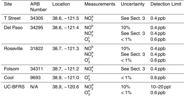
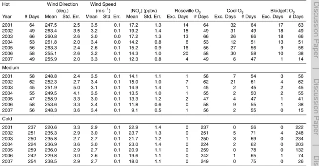
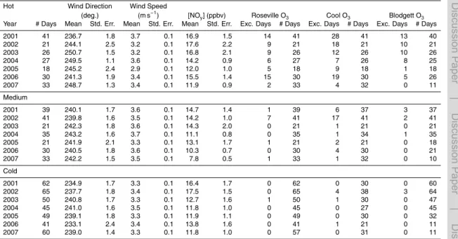
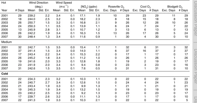
Seven years of NOx and O3data were compiled from three CARB sites (Del Paso, Roseville, and Cool) (CARB, 2009) and from UC Berkeley measurements at UC-BFRS between 2001 and 2007. Table 1 summarizes the observations used from each site and the methods of detection. These four sites fall roughly along the center line of the plume and split the transect into three segments that will be referred to as Segments A
5
(Del Paso to Roseville), B (Roseville to Cool), and C (Cool to UC-BFRS). Temperature and solar radiation measurements from the California Irrigation Management Informa-tion System site at Fair Oaks, located roughly in between Del Paso and Roseville, and wind speed and wind direction from the Camino CIMIS site located to the southwest of UC-BFRS (CIMIS, 2009). Table 2a summarizes the full 7 year data set.
10
The method for NOx detection at the CARB sites is the catalytic conversion of NO2 to NO, followed by detection of total NO (ambient plus converted) by chemilumines-cence. Subtraction of the NO signal detected in ambient air from the NOxsignal gives the response, labeled “NO2.” There are known positive artifacts to this measurement (Winer et al., 1974; Grosjean and Harrison, 1985; Dunlea et al., 2007; Steinbacher et
15
al., 2007) as a result of the accompanying conversion of peroxy nitrates (PNs), alkyl & multifunctional alkyl nitrates (ANs), and nitric acid (HNO3) over the molybdenum oxide (MoO) catalytic converter. In this study, we will assume that these higher oxides are detected with 100% efficiency and refer to observations reported as “NOx” by CARB, instead, as NOy.
20
For the purpose of understanding the role of NOxin Ox chemistry, we estimate NOx mixing ratios from the observations of NOy. To do this we assume that the sum of the higher oxides of nitrogen are present at the monitoring stations in an amount equal to the NO2 at those stations (a ratio roughly consistent with observations of NO2, PNs, ANs and HNO3 at the Granite Bay site – Cleary et al., 2005; Cleary et al., 2007).
25
ACPD
11, 6259–6299, 2011Temperature dependent response
of ozone to NOx
B. W. LaFranchi et al.
Title Page
Abstract Introduction
Conclusions References
Tables Figures
◭ ◮
◭ ◮
Back Close
Full Screen / Esc
Printer-friendly Version Interactive Discussion
Discussion
P
a
per
|
Dis
cussion
P
a
per
|
Discussion
P
a
per
|
Discussio
n
P
a
per
|
observed “NO2”.
Based on the average daily wind speed, the Lagrangian plume age, relative to an arbitrary start time (to), can be approximated for each measurement site along the
transect. Selecting Del Paso as the plume start point and atoof 1000 PST, the plume passes over Roseville, Cool, and UC-BFRS at 1200 PST, 1500 PST, and 1700 PST
5
respectively. Daily values for each available measurement were obtained from 2 h averages about these times.
Equation (4) is solved for∆[Ox]chem/∆tfor each plume segment using a constant O3 background of 53 ppb (NO2background is negligible for consideration of odd-oxygen) and kmix=0.31 h−1 (see Appendix B for details). Since there are no nitrogen oxide
10
measurements available at the Cool site, we estimate NOy (and NOx) based on an exponential decay from Roseville with a lifetime of 2 h and a transit time of 3 h. The resulting NOx is consistent with observations of NOx further downwind at UC-BFRS and amounts to NO2levels of at most 3% of Ox at the site.
The analysis is applied to the months of May through September and uses days
15
when wind speeds are between 3 and 4 m s−1(at the Camino site), wind direction is W or SW (between 200 and 260 degrees, at Camino), and solar radiation is within 10% of a 30 day running mean (at Fair Oaks) to ensure clear sky conditions. About half of the observations from May through September survive this filter. There is no significant correlation of wind speed or wind direction with temperature or NOy in this data set
20
(R2<0.04). The filtered data used in this analysis is summarized in Table 2c.
4 Observed NOxand Temperature influence on P(Ox)
Figure 2 shows the annual average NOy observed during the summer months (May– September, 2001–2008) from the average of 4 GSA monitoring sites (T Street, Del Paso, Roseville, and Folsom). Observations are shown for all days, weekdays only,
25
ACPD
11, 6259–6299, 2011Temperature dependent response
of ozone to NOx
B. W. LaFranchi et al.
Title Page
Abstract Introduction
Conclusions References
Tables Figures
◭ ◮
◭ ◮
Back Close
Full Screen / Esc
Printer-friendly Version Interactive Discussion
Discussion
P
a
per
|
Dis
cussion
P
a
per
|
Discussion
P
a
per
|
Discussio
n
P
a
per
|
of 0.6–0.7 ppb year−1. This long-term decrease is of the same magnitude as the mean observed weekday-weekend difference over the study period (∼5 ppb). The day-of-week effect in the Sacramento region has also been observed in the satellite record (Russell et al., 2010) and was found to have a significant effect on ozone production rates, as reported by Murphy et al. (2006b; 2007).
5
It is our expectation that the primary variables causing changes in ozone production rates are the NOx and biogenic VOC concentrations. Since BVOCs are emitted as an exponential function of temperature, we use temperature as a surrogate to represent changes in VOC reactivity. Changes in radical propagating reaction rates and water vapor are expected to be correlated with changes in temperature and BVOC emissions.
10
These factors also have an impact on ozone production rates although their effects are smaller than those of BVOCs (Steiner et al., 2006).
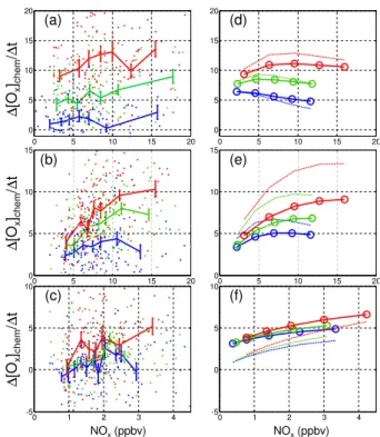
Figure 3a–c show∆[Ox]chem/∆tfor each segment vs NOx estimated from measure-ments at the upwind site and in three different temperature regimes (low, medium, and high). For Segment A (Fig. 3a), the region between Del Paso and Roseville,
15
∆[Ox]chem/∆t increases with both temperature and NOx. The slope of ∆[Ox]chem/∆t vs NOx increases as temperature increases. Figure 3b shows the behavior of
∆[Ox]chem/∆t between Roseville and Cool (Segment B). As in Fig. 3a, Ox production rates are sensitive to both NOx and temperature. At the low NOx end, however, the temperature dependence is minimal. Additionally, the NOxdependence is a nonlinear
20
function of NOx with a steeper variation at lower NOx concentrations, particularly for the medium and high temperature bins. The segment between Cool and UC-BFRS has much lower NOx concentrations. The∆[Ox]chem/∆t in this segment (Fig. 3c) shows a slight increase with NOx, but no discernable temperature dependence, except at the highest NOx concentrations. Net Ox production rates inferred from observations are
25
ACPD
11, 6259–6299, 2011Temperature dependent response
of ozone to NOx
B. W. LaFranchi et al.
Title Page
Abstract Introduction
Conclusions References
Tables Figures
◭ ◮
◭ ◮
Back Close
Full Screen / Esc
Printer-friendly Version Interactive Discussion
Discussion
P
a
per
|
Dis
cussion
P
a
per
|
Discussion
P
a
per
|
Discussio
n
P
a
per
|
5 Comparison of observed ozone production with two models
The qualitative patterns of P(Ox) as a function of NOx and temperature shown in Fig. 3a–c are consistent with predictions based on standard photochemistry. Here we make use of equations describing instantaneous Ox production derived by Murphy et al. (2006b). Briefly, O3participates in a null catalytic cycle with nitrogen radicals (NO
5
and NO2). As a result, Ox is more conserved than either individually. This so called NOxcycle is described by Reactions (R1) to (R3).
O3+NO→NO2+O2 (R1)
NO2+hν→O+NO (R2)
O+O2→O3 (R3)
10
Net Ox production occurs when some alternative oxidant facilitates the conversion of NO to NO2. In continental regions, this is most often achieved through the oxidation of volatile organic compounds (VOCs). Reactions (R4)–(R7) outline the oxidation of VOCs by the hydroxyl radical (OH) and subsequent reaction of peroxy radicals with NO (R5 and R7), which, when coupled with NO2 photolysis (R2 and R3), leads to net
pro-15
duction of O3 during the daytime. This series of reactions is radical propagating, with no net loss of NOx or HOx taking place. The rate of Ox production can be calculated as the combined rates of Reactions (R5 and R7), or as approximately twice the rate of any single reaction in this cycle.
OH+VOC(+O2)→RO2+H2O (R4)
20
RO2+NO→NO2+RO (R5)
RO+O2→R′O+HO2 (R6)
ACPD
11, 6259–6299, 2011Temperature dependent response
of ozone to NOx
B. W. LaFranchi et al.
Title Page
Abstract Introduction
Conclusions References
Tables Figures
◭ ◮
◭ ◮
Back Close
Full Screen / Esc
Printer-friendly Version Interactive Discussion
Discussion
P
a
per
|
Dis
cussion
P
a
per
|
Discussion
P
a
per
|
Discussio
n
P
a
per
|
Accompanying these propagating reactions are a series of radical terminating Reac-tions, (R8)–(R12), which ultimately limits P(Ox) through their influence on the concen-trations of the reactants in (R4)–(R7). These terminating reactions are thought of in two categories, one involving self-reactions of peroxy radicals (HOx–HOxReactions, (R8)– (R10)), and one involving cross reactions between NOx and HOx radicals (NOx–HOx
5
Reactions, (R11) and (R12)).
HO2+HO2→H2O2+O2 (R8)
HO2+RO2→ROOH+O2 (R9)
RO2+RO2→non-radical products (R10)
NO2+OH→HNO3 (R11)
10
NO+RO2→RONO2 (R12)
The distinction between these two types of radical terminating reactions is what leads to different ozone production regimes, giving rise to NOx-limited and NOx-suppressed or VOC-limited behavior (e.g. Sillman et al., 1990; Sillman, 1995). Non-linearities arise in the relationship between ozone production and the primary ozone precursors, NOx
15
and VOCs, as a result of OH suppression by NO2 at high NOx (Reaction (R11)) and peroxy radical self reactions that limit their abundance at low NOx (Reactions (R8)– (R10)).
P(Ox) can be calculated over a range of [NOx], VOC reactivities, and temperature by simultaneously solving steady-state equations for OH, HO2, and RO2species at each
20
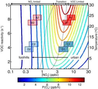
input value (Kleinman et al., 1997; Thornton et al., 2002; Murphy et al., 2006b). Fig-ure 4 shows the results from such a calculation, where P(Ox) is plotted as a function of [NOx], and against two correlated variables: VOC reactivity (Σki[VOC]i) on the left axis and temperature on the right axis. Additional reactions included in this particular calcu-lation, not listed in the reaction series (R1)–(R12), are the radical propagating reactions
ACPD
11, 6259–6299, 2011Temperature dependent response
of ozone to NOx
B. W. LaFranchi et al.
Title Page
Abstract Introduction
Conclusions References
Tables Figures
◭ ◮
◭ ◮
Back Close
Full Screen / Esc
Printer-friendly Version Interactive Discussion
Discussion
P
a
per
|
Dis
cussion
P
a
per
|
Discussion
P
a
per
|
Discussio
n
P
a
per
|
of OH+CO and O3+HO2and the photolysis of O3and formaldehyde. The relevant pa-rameters for this calculation, tailored to observations in the Sacramento urban plume, are: NO2/NO=4.5; [CO]=140 ppbv; [O3]=53 ppbv; P(OH)=5×10
6
molec cm−3s−1; P(HO2)=5×10⁶molec cm−3s−1; alkyl nitrate branching ratio α =k
12/k5) 5%; [M]=2.45×10¹⁹molec cm−3. As is well known, three different photochemical regimes
5
can be identified in these non-linear equations, a NOx limited regime where Ox pro-duction increases with increasing NOx and is insensitive to VOC, a NOx suppressed or VOC limited regime where Ox production decreases with increases in NOx and in-creases with increasing VOC reactivity, and a transition regime where production is relatively insensitive to changes in either parameter.
10
Also shown in Fig. 4 are shaded boxes representing NOx concentrations in the Sacramento urban plume. The boxes show the range (inter-quartile) of concentra-tions observed in the metropolitan Sacramento region (average of 4 sites, as in Fig. 2) and the resulting concentrations in the plume after 5 h of aging, assuming a 2 h NOx lifetime due to the combined effects of oxidation and dilution. The boxes represent
av-15
erage plume conditions in the years 2001 (A and C) and 2007 (B and D) under high (red) and low (blue) temperature scenarios. To the extent that this calculation, which represents perpetual noon, can simulate the time over which Ox is produced, we in-terpret Fig. 4 as a prediction for the response of P(Ox) to advection and dilution of the plume. In the early years of the study period, on both weekdays and weekends and at
20
all temperatures, the urban initialization of the plume begins to the right of the ridge-line, clearly in the NOxsuppressed (VOC limited) regime. The plume always ends up well in the NOxlimited regime. By 2007, decreases in NOxemissions have resulted in initial conditions that are essentially right at the ridgeline. The model also predicts that increases in temperature, at constant NOx and with corresponding increases in VOC
25
ACPD
11, 6259–6299, 2011Temperature dependent response
of ozone to NOx
B. W. LaFranchi et al.
Title Page
Abstract Introduction
Conclusions References
Tables Figures
◭ ◮
◭ ◮
Back Close
Full Screen / Esc
Printer-friendly Version Interactive Discussion
Discussion
P
a
per
|
Dis
cussion
P
a
per
|
Discussion
P
a
per
|
Discussio
n
P
a
per
|
We use Fig. 4 to interpret ∆[Ox]chem/∆t as shown in Fig. 3. In the early plume evolution (Segment A)∆[Ox]chem/∆t increases with temperature at all NOx values. In the low temperature range, there is not a significant trend with NOx, while there is a clear increase with NOx in the middle and high temperature bins. Comparing to the trends one would expect by integrating Fig. 4 during dilution (i.e. along the arrow
5
shown), we interpret the observations as indicating that this region of the plume is NOx limited. The data show that changes in VOC influence ozone production rates in roughly the manner expected – we observe steep increases with increasing VOC. NOx increases result in small increases or almost no change in∆[Ox]chem/∆t, perhaps an indication that the trajectory of the first segment moves the plume through the ridgeline,
10
or perhaps an effect of added urban sources of VOC emissions that correlate with NOx. In segment B of the plume, where it moves from Roseville to Cool, our analysis (Fig. 3b) shows an increase in P(Ox) at low NOx and a slow in the increase at the highest NOx. We interpret this slower rate of increase in P(Ox) at high NOxin Segment B to indicate that this segment of the plume crosses over the transition region into
15
NOx-limited Oxproduction. The temperature dependence of∆[Ox]chem/∆tis additional evidence that these first two segments are VOC limited. As seen in the model (Fig. 4) at fixed NOx, O3production contours are a strong function of temperature. In contrast, further downwind, in Segment C, we observe a increase in∆[Ox]chem/∆twith NOxthat is independent of temperature indicating this segment of the plume is NOxlimited.
20
The qualitative interpretation of the ∆[Ox]chem/∆t as a function of temperature and NOxis supported by a more quantitative analysis using a 1-D Lagrangian plume model with detailed chemistry. A brief description of the model and details particular to this work are given in Appendix A. A complete description of the model can be found in Perez (2008) and Perez et al. (2009). This model represents diurnal variations that
25
ACPD
11, 6259–6299, 2011Temperature dependent response
of ozone to NOx
B. W. LaFranchi et al.
Title Page
Abstract Introduction
Conclusions References
Tables Figures
◭ ◮
◭ ◮
Back Close
Full Screen / Esc
Printer-friendly Version Interactive Discussion
Discussion
P
a
per
|
Dis
cussion
P
a
per
|
Discussion
P
a
per
|
Discussio
n
P
a
per
|
from the model in the same manner as from the observations – taking the Oxdifference between the beginning and end points of each segment and adjusting for the effect of dilution.
This model calculation has a remarkable correspondence to the patterns in the ob-servations. For segment A, the model calculation shows three more or less flat and
5
parallel lines that are well separated; for segment B, the model calculation shows cur-vature that is very much like the observations; and for segment C the model shows three curves that are almost on top of one another indicating that∆[Ox]chem/∆tis inde-pendent of VOC and temperature in this region a result virtually identical to the analysis of the observations.
10
This is not to say the correspondence is perfect. ∆[Ox]chem/∆t in the model is too strongly NOxsuppressed in the first segment. The observations have a slightly positive slope while the model slightly negative. In segment B, ∆[Ox]chem/∆t doesn’t rise as steeply as the observations or reach values as high. In segment C, the net production at the lowest NOxis much higher than in the observations. However, our point here is
15
not to establish that this model is correct, but rather to establish that this method of analysis of the observations does provide a strong challenge to any model, one that is especially sensitive to Oxproduction chemistry.
Some of the model observation differences can be interpreted as due to the model not having the ridgeline between NOx limited and NOx suppressed behavior in the
20
right location. Factors that influence the location of this the boundary and thus may contribute to the model/observation discrepancy are: (1) uncertainty in the modeled VOC reactivity, for which very few observations exist in the region; a doubling of VOC reactivity in the model increases the NOx concentration where P(Ox) peaks by about 50% and would result in better agreement of the model and observations, (2)
uncer-25
ACPD
11, 6259–6299, 2011Temperature dependent response
of ozone to NOx
B. W. LaFranchi et al.
Title Page
Abstract Introduction
Conclusions References
Tables Figures
◭ ◮
◭ ◮
Back Close
Full Screen / Esc
Printer-friendly Version Interactive Discussion
Discussion
P
a
per
|
Dis
cussion
P
a
per
|
Discussion
P
a
per
|
Discussio
n
P
a
per
|
et al., 2010); observations of higher oxides of nitrogen as a function of temperature by Day et al. (2008) also indicated a need for additional OH in the region. An increase in OH by a factor of 2 would increase the modeled transition point between NOx-limited and NOx-suppressed ozone production by 25%, resulting in slightly better agreement between observations and the model; and (3) the uncertainty in our assumptions about
5
the fraction of observed “NO2” in the urban core that is true NO2, which we estimate at 50–70%; if NO2 is a smaller fraction of the observed NO2 than we estimate, the perceived transition point would occur at lower NOx.
6 Implications for regional air quality
Regional air quality is a function of the integrated ozone production over the entire
10
plume, P(Ox)tot. From Fig. 4, an increase in temperature, and, consequently, VOC reactivity, is predicted to increase P(Ox) in the urban core, leading to an overall increase in P(Ox)tot with temperature at all points in the plume, despite having little impact on P(Ox) in the NOx-limited foothills. A reduction in NOx emissions in the urban core, as observed in 2007 relative to 2001, may not have a significant effect on P(Ox) in the
15
early stages of the plume or may even result in increased O3 in the urban core, but the point of peak ozone production and then NOx-limiting behavior will be achieved closer to the urban core and P(Ox)tot will decrease. This will be especially apparent at higher temperatures (higher BVOC emissions), where the P(Ox) contours are a steeper function of NOx, as illustrated in Fig. 4. Thus, it is expected that the reductions in NOx
20
that occurred over the period of 2001 to 2007 were more effective at reducing O3levels at high temperatures, where P(Ox) is highest, than at low temperatures.
Our analysis of ∆[Ox]chem/∆t above reinforces these model-based predictions for P(Ox) in the Sacramento urban plume as a function of distance from the urban core, temperature, and NOx. Comparison of these predictions of P(Ox) as a function of NOx
25
ACPD
11, 6259–6299, 2011Temperature dependent response
of ozone to NOx
B. W. LaFranchi et al.
Title Page
Abstract Introduction
Conclusions References
Tables Figures
◭ ◮
◭ ◮
Back Close
Full Screen / Esc
Printer-friendly Version Interactive Discussion
Discussion
P
a
per
|
Dis
cussion
P
a
per
|
Discussion
P
a
per
|
Discussio
n
P
a
per
|
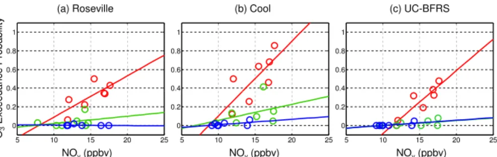
standard (90 ppb) on any given day during calendar years 2001–2007 provides useful insight. By focusing on the exceedance probability, variability in the annual distribu-tion of high, medium, and low temperature days from year to year is removed, and the effects of the steady decline in NOxemissions can be quantified. This probability is cal-culated for three different temperature bins and plotted against the annual region-wide
5
average NOy mixing ratio in Fig. 5a (Roseville), b (Cool), and c (UC-BFRS). For these probability calculations, a meteorological filter (similar to that described in Sect. 3) is used to select a subset of observation days during the ozone season. In a given year, somewhere between 60% and 90% of the observation days survive this filter. Table 2b summarizes the data used in these calculations. The uncertainty in the exceedance
10
probability is calculated as 1/2√N/N, whereN is the total number of days in each tem-perature bin for a given year. Typical uncertainties in the exceedance probability in a given year are about±0.1 (1σ).
A dramatic effect in the exceedance probability is observed at Cool, where, in 2001 when the annual average NOy in the urban core was 18 ppb, nearly 70% of the days
15
with a maximum air temperature of at least 33◦C were over the exceedance limit; but in 2007 at an urban NOyconcentration of 12 ppb only 10% of these days exceeded the limit (Fig. 5b). At Roseville (Fig. 5a) the sensitivity to NOy decreases is lower than at Cool, but still quite strong. The data show a change in exceedance probability during the hot days from about 40–50% in the early part of the study period to 10–20% in
20
the later part. Finally, at UC-BFRS, reductions in NOx emissions in the Sacramento Metro region have reduced the exceedance probability at UC-BFRS, some 90 km to the northeast, from 50% to 0% on high temperature days (Fig. 5c). There are also reductions at lower temperatures, which are most evident at Cool.
Early in the study period, the number of exceedance days each year at UC-BFRS
25
ACPD
11, 6259–6299, 2011Temperature dependent response
of ozone to NOx
B. W. LaFranchi et al.
Title Page
Abstract Introduction
Conclusions References
Tables Figures
◭ ◮
◭ ◮
Back Close
Full Screen / Esc
Printer-friendly Version Interactive Discussion
Discussion
P
a
per
|
Dis
cussion
P
a
per
|
Discussion
P
a
per
|
Discussio
n
P
a
per
|
the downwind regions, as outlined by Murphy et al. (2007). Nonetheless, the 30% decrease in NOy that occurred from 2001 to 2007 has been extremely effective in reducing the exceedance probability at all locations during the hottest days of the year when increases in biogenic emissions result in chemistry that shifts to conditions that are more NOx limited. To put these results in perspective, if NOy levels in 2007 had
5
remained at 2001 levels, the 33 high temperature days during 2007 are predicted to have resulted in 22 (±5) exceedance days at Cool, instead of the 4 that actually did occur.
It has been argued (e.g. Muller et al., 2009) that NOxdecreases cause O3increases in the center of cities and are more detrimental to health because of the larger number
10
of people who live in the urban core as opposed to the surrounding suburbs and rural regions. In GSA, Murphy et al. (2007) found that O3 concentrations (8 h maximum) increased on weekends in the urban core during the time period of 1998–2002 as a response to decreases in NOx of approximately 20% on weekends. We find that between 2001 and 2007, the average O3 is higher on weekends than on weekdays
15
only for the lowest temperature days. Because O3 concentrations on low temperature days are generally well below the exceedance limit, increases in O3 with decreasing NOx are not likely to lead to additional exceedances. Thus, we find no evidence that implementation of NOx emission controls has been detrimental to air quality, by any policy-relevant metric, at any of the sites considered in this analysis over the period
20
2001 through 2007 (and presumably up to the present day).
We calculate a projected time frame for eliminating exceedances in the region using the data in Fig. 5 to extrapolate to a 0% exceedance probability. We calculate both a 50% confidence time-frame, from the mean exceedance probabilities and a 95% con-fidence time frame, from the upper bound of the 2σuncertainty in the mean. The high
25
ACPD
11, 6259–6299, 2011Temperature dependent response
of ozone to NOx
B. W. LaFranchi et al.
Title Page
Abstract Introduction
Conclusions References
Tables Figures
◭ ◮
◭ ◮
Back Close
Full Screen / Esc
Printer-friendly Version Interactive Discussion
Discussion
P
a
per
|
Dis
cussion
P
a
per
|
Discussion
P
a
per
|
Discussio
n
P
a
per
|
by 2018. Using a 50% confidence criteria, decreases in NOy expected to be achieved by 2012 (30%) will result in zero exceedances.
Climate change is expected to result in higher average temperatures in California, increasing biogenic VOC emissions by 15–35% in the Sacramento region by 2050 (Steiner et al., 2006). Absent reductions in NOx, an increase in the number of high
5
temperature days would increase the average integrated P(Ox) in the plume and in-crease the probability of exceeding the 1 h O3standard in a given year. Between 2001 and 2007, there were on average 28±7 high temperature days per year. An increase in the number of hot days would likely increase the number of exceedances; however, even a doubling of the number of annual high temperature days over the next ten years
10
is not expected to extend the projected time frames (50% and 95%) for eliminating ex-ceedances by more than a year. Therefore, unless there is a significant departure from the projected rate of decrease in NOx emissions, increased high temperature days are not expected to affect the number of O3exceedances, in the next few decades.
An additional consideration for predicting the decline in O3 exceedance days is the
15
reported rise in the global tropospheric O3background. Parrish et al. (2009) estimate that background Ox in air transported across the Pacific has been increasing at a rate of 0.46 ppb year−1. If we increase the O3 observed in 2007 by 5 ppb to simulate an upper limit to the effect of this increase in background O3 after 10 years, we estimate mixing of this larger background would have the effect of increasing the frequency of
20
violations at high temperature from 6% (in 2007) to 9% at Roseville and from 13% to 30% at Cool, with no further decrease in NOx. However, we note that the increase reported by Parrish et al. (2009) would be largest in the recent years when NOx is lowest. Were it a strong effect we would expect to see a slowing of the decrease in exceedance probability at lower NOx. We do not, a result we believe indicates growth
25
ACPD
11, 6259–6299, 2011Temperature dependent response
of ozone to NOx
B. W. LaFranchi et al.
Title Page
Abstract Introduction
Conclusions References
Tables Figures
◭ ◮
◭ ◮
Back Close
Full Screen / Esc
Printer-friendly Version Interactive Discussion
Discussion
P
a
per
|
Dis
cussion
P
a
per
|
Discussion
P
a
per
|
Discussio
n
P
a
per
|
7 Conclusions
We have presented a quantitative method for evaluating the NOx and temperature de-pendence of Oxproduction in an urban plume. The observational analysis represents a direct test of model chemistry. O3 exceedance days at all points in the plume are observed to have a strong temperature dependence (Fig. 5) due to the persistence in
5
the plume of O3produced in the urban core and suburbs. We show that the 30% de-crease in NOx over the time frame of 2001 to 2007 has lead to a significant decrease in O31-h exceedance days region-wide, especially during the hottest days. The reduc-tion in exceedance days has been most significant at the farthest downwind regions of the plume. We predict that an additional decrease in NOx will effectively eliminate
10
O3 1-h exceedances in the region. At the current rate of the observed NOy decrease (Fig. 2), we predict with 50% confidence that exceedances will end in 2012 and with 95% confidence that exceedances will be eliminated in the region by 2018.
Appendix A
15
Lagrangian urban plume model
A detailed description of the Lagrangian model of the Sacramento urban plume is given in Perez (2008) and Perez et al. (2009). The model represents mixing, photochemistry, and dry deposition as occurring in a box that is transported from Granite Bay, located close to Roseville, to UC-BFRS at a rate set by the local winds. The chemical
mecha-20
nism is a reduced form of the Master Chemical Mechanism (v 3.1) with modifications as outlined in Perez et al. (2009). There are a total of 370 reactions, 170 specific chemicals, and 7 lumped species in the model.
The model is initialized with observations at Granite Bay at noon and propagated for-ward along the Lagrangian plume coordinates in space and time. To the east of Granite
25
ACPD
11, 6259–6299, 2011Temperature dependent response
of ozone to NOx
B. W. LaFranchi et al.
Title Page
Abstract Introduction
Conclusions References
Tables Figures
◭ ◮
◭ ◮
Back Close
Full Screen / Esc
Printer-friendly Version Interactive Discussion
Discussion
P
a
per
|
Dis
cussion
P
a
per
|
Discussion
P
a
per
|
Discussio
n
P
a
per
|
including isoprene, MBO, and terpenes are based on Steiner et al. (2006). Biogenic NOx emissions are estimated from measured fluxes of soil NOx in the oak forests of the Sierra Nevada foothills (Herman et al., 2003). At characteristic wind speeds, the plume passes over Cool after 3 h and reaches UC-BFRS after 5 h. In order to simulate the range of conditions observed, the model is run at 3 different temperatures and 5
5
different initial NOx(and NOy) concentrations for a total of 15 separate model runs. The model inputs are variable with temperature according to the Granite Bay observations in 2001. On top of this temperature variability, the NOx and NOy inputs are artificially scaled by factors of 0.33, 0.66, 1, 1.33, and 1.66 to provide 5 different NOx scenarios for each temperature scenario.
10
Model outputs consist of concentrations of all species at 2 min intervals along the plume transect. The model output can be compared directly to the observations of
∆[Ox]chem/∆t between Roseville and Cool (first 3 h of plume age) and between Cool and UC-BFRS (last 2 h of plume age). In order to simulate the segment between Del Paso and Roseville, the model is modified to start at 1000 PST, and anthropogenic
15
emissions are simulated for the first 2 h of the transect. Equation (4) is used to calcu-late ∆[Ox]chem/∆t from the model outputs in an identical manner to that used on the observations. An important advantage to using the model is that P(Ox) can be calcu-lated directly and compared to the net chemical flux of Ox as calculated by Eq. (4) in order to understand where this approach might be affected by biases when applied to
20
the observations.
Appendix B
Entrainment of background air
For calculating∆[Ox]chem/∆t, entrainment of background air into the plume is treated
25
ACPD
11, 6259–6299, 2011Temperature dependent response
of ozone to NOx
B. W. LaFranchi et al.
Title Page
Abstract Introduction
Conclusions References
Tables Figures
◭ ◮
◭ ◮
Back Close
Full Screen / Esc
Printer-friendly Version Interactive Discussion
Discussion
P
a
per
|
Dis
cussion
P
a
per
|
Discussion
P
a
per
|
Discussio
n
P
a
per
|
plume where mixing occurs at the top of the boundary layer with free tropospheric air. Perez et al. (2009) found that the model best reproduced observations when a low “Global” background was used, characteristic of free troposphere air. Under this scenario, a constant O3 background of 53 ppb is assumed. The mixing rate of the plume (kmix) under these conditions was calculated to be 0.31 h−
1 .
5
Changes in the absolute values of the mixing parameters, including the entrain-ment rate and the O3 background, are expected to influence the absolute values of
∆[Ox]chem/∆t, but not the observed relationships with temperature and [NOx]. Uncer-tainty in thevariability of the entrainment rate or the background concentration of O3, however, could potentially bias our results in a way that would artificially introduce a
10
temperature dependence to∆[Ox]chem/∆t.
Parrish et al. (2010) found a correlative link between O3 in background air arriving at the coast of northern California from the west and high O3concentrations observed in certain locations of the Central Valley 22 h later. While the role of temperature was not specifically addressed in this study, the observations of Parrish et al. (2010) imply
15
that the relevant [O3]bkvalue for our analysis should be higher when temperatures are higher. Similarly, if there is a carryover effect from day to day, and [O3]bk has some dependence on the chemistry occurring in the boundary layer on the previous day in the Central Valley, it would likely be positively correlated with temperature since warm days generally follow other warm days.
20
Under each of these scenarios, higher temperatures, and a corresponding higher ozone background, would lead to a slower rate of dilution for Ox in the plume and a lower inferred value for∆[Ox]chem/∆t. To understand the potential impact of this on our results, we recalculate∆[Ox]chem/∆t, using a temperature dependent Ox background, calculated as a linear function of temperature and normalized such that the average
25
ACPD
11, 6259–6299, 2011Temperature dependent response
of ozone to NOx
B. W. LaFranchi et al.
Title Page
Abstract Introduction
Conclusions References
Tables Figures
◭ ◮
◭ ◮
Back Close
Full Screen / Esc
Printer-friendly Version Interactive Discussion
Discussion
P
a
per
|
Dis
cussion
P
a
per
|
Discussion
P
a
per
|
Discussio
n
P
a
per
|
the absolute values of∆[Ox]chem/∆tat the high and low temperatures, but the basic fea-tures of the inferred relationship between ozone production, NOx, and temperature are unchanged at all three segments of the transect. We find that an unreasonably large variability in [O3]bk(likely a range of 35 ppb or greater), that is perfectly correlated with temperature, would be necessary to produce the observed behavior in∆[Ox]chem/∆t
5
with temperature.
Similarly, any relationship of the plume entrainment rate with temperature could give rise to a dampening of the perceived dependence of∆[Ox]chem/∆ton temperature. This would occur if the entrainment rate slowed with increasing temperature. A conservative upper limit for this effect was estimated previously from correlations between CO, NOy,
10
and temperature at UC-BFRS (Day et al., 2008); at this limit, no more than a 20% increase in NOy at UC-BFRS could be accounted for by a slowing of the entrainment rate with increased temperatures in the Sacramento urban plume. In our analysis, varying the entrainment rate by±20% (negatively correlated with temperature), which is more than sufficient to induce a 20% change in NOy at UC-BFRS, does not change
15
the patterns of∆[Ox]chem/∆t with NOxand temperature appreciably.
Appendix C
The role of anthropogenic VOCs
In our analysis we have assumed that the VOC reactivity at all points along the plume is
20
dominated by biogenic emissions and their oxidation products. Observations at Gran-ite Bay and UC-BFRS support this contention (Lamanna and Goldstein, 1999; Cleary et al., 2005; Steiner et al., 2008) for the suburbs and foothills. While observations of a detailed set of VOCs closer to the urban core are lacking, Steiner et al. (Steiner et al., 2008) used the CMAQ model (with a 4 km horizontal resolution) to predict about equal
25
ACPD
11, 6259–6299, 2011Temperature dependent response
of ozone to NOx
B. W. LaFranchi et al.
Title Page
Abstract Introduction
Conclusions References
Tables Figures
◭ ◮
◭ ◮
Back Close
Full Screen / Esc
Printer-friendly Version Interactive Discussion
Discussion
P
a
per
|
Dis
cussion
P
a
per
|
Discussion
P
a
per
|
Discussio
n
P
a
per
|
primary source of VOCs in the region, including in the urban core, have a strong tem-perature dependence. Presumably a major fraction of these temtem-perature-dependent compounds are biogenics. It has been shown that evaporative anthropogenic VOC emissions can be significant in many urban locations (Rubin et al., 2006), but their contribution to the total VOC reactivity in the region is minimal compared to either the
5
anthropogenic fuel combustion or biogenic VOC sources.
Strict regulations have resulted in a dramatic reduction of reactive VOCs in urban regions throughout California since the mid 1970s (Cox et al., 2009). According to CARB, anthropogenic VOC emissions, including those from evaporative sources, con-tinued to decrease between 2000 and 2005 in the Sacramento Valley Air Basin at a
10
rate of about 3% per year, similar to that reported for NOx emissions over the same time frame (Cox et al., 2009). The likely correlation between NOx and anthropogenic VOCs in the long-term data set begs the question: to what extent are the perceived reductions in P(Ox) with NOxdue to the accompanying changes in anthropogenic VOC emissions? This effect would be most prevalent in the region between Del Paso and
15
Roseville, where ozone production is most sensitive to VOC concentrations and where anthropogenic VOC emissions are expected to be greatest.
The realization of NOx reductions across two different time-scales, both interannual and day-of-week, allows us to address this question. The day-of-week changes in NOx concentrations are thought to be primarily due to changes in the number of
com-20
mercial diesel vehicles on the road from weekdays to weekends (Harley et al., 2005; Murphy et al., 2007). Since VOC emissions from diesel engines are a small fraction of total anthropogenic VOC emissions, day-of-week variability in VOC emissions are not expected to be correlated with NOx. Conversely, over inter-annual time-scales, NOx reductions have come primarily as a result of cleaner gasoline vehicles replacing older
25
ACPD
11, 6259–6299, 2011Temperature dependent response
of ozone to NOx
B. W. LaFranchi et al.
Title Page
Abstract Introduction
Conclusions References
Tables Figures
◭ ◮
◭ ◮
Back Close
Full Screen / Esc
Printer-friendly Version Interactive Discussion
Discussion
P
a
per
|
Dis
cussion
P
a
per
|
Discussion
P
a
per
|
Discussio
n
P
a
per
|
Thus, a simple test of whether reductions in VOC emissions over the long term have had a significant impact on ozone production rates is to compare∆[Ox]chem/∆tvalues from the early part of the study period (2001–2002) to the later part (2006–2007) under conditions where NOx mixing ratios and temperatures are comparable. We find that there is no significant difference in the calculated ∆[Ox]chem/∆t values between the
5
early period and the late period of the analysis time frame at similar temperatures and NOx. We conclude, therefore, that there is no evidence of decreased P(Ox) between 2001 and 2007 resulting from decreases in anthropogenic VOC emissions. This comes despite a nearly equal relative decrease in VOC and NOxemissions (Cox et al., 2009) over this time and implies that the intensity of biogenic VOC emissions have made NOx
10
emission reductions more effective than anthropogenic VOC emission reductions in the region, at least downwind of Del Paso.
Acknowledgements. The authors thank the UC Blodgett Forest Research Station stafffor logis-tical support, Sierra Pacific Industries for access to their land, Megan McKay for maintenance of the measurement site and data, and Rynda Hudman for helpful discussions. We would also like
15
to acknowledge the California Air Resources Board and the California Irrigation Management System for making their data publicly available. This work was supported by the National Sci-ence Foundation (grant ATM-0639847). B. LaFranchi acknowledges support from the Camille and Henry Dreyfus Postdoctoral Program in Environmental Chemistry. A portion of this work was performed under the auspices of the US Department of Energy by Lawrence Livermore
20
National Laboratory under Contract DE-AC52-07NA27344.
References
Archibald, A. T., Cooke, M. C., Utembe, S. R., Shallcross, D. E., Derwent, R. G., and Jenkin, M. E.: Impacts of mechanistic changes on HOx formation and recycling in the oxidation of isoprene, Atmos. Chem. Phys., 10, 8097–8118, doi:10.5194/acp-10-8097-2010, 2010.
25
ACPD
11, 6259–6299, 2011Temperature dependent response
of ozone to NOx
B. W. LaFranchi et al.
Title Page
Abstract Introduction
Conclusions References
Tables Figures
◭ ◮
◭ ◮
Back Close
Full Screen / Esc
Printer-friendly Version Interactive Discussion
Discussion
P
a
per
|
Dis
cussion
P
a
per
|
Discussion
P
a
per
|
Discussio
n
P
a
per
|
Ban-Weiss, G. A., McLaughlin, J. P., Harley, R. A., Lunden, M. M., Kirchstetter, T. W., Kean, A. J., Strawa, A. W., Stevenson, E. D., and Kendall, G. R.: Long-term changes in emissions of nitrogen oxides and particulate matter from on-road gasoline and diesel vehicles, Atmos. Environ., 42, 220–232, doi:10.1016/j.atmosenv.2007.09.049, 2008.
Bouvier-Brown, N. C., Goldstein, A. H., Gilman, J. B., Kuster, W. C., and de Gouw, J. A.:
In-5
situ ambient quantification of monoterpenes, sesquiterpenes, and related oxygenated com-pounds during BEARPEX 2007: implications for gas- and particle-phase chemistry, Atmos. Chem. Phys., 9, 5505–5518, doi:10.5194/acp-9-5505-2009, 2009.
California Air Resources Board Air Quality Database: http://www.arb.ca.gov/aqd/aqdcd/aqdcd. htm, last access: September 15, 2009.
10
Carroll, J. J. and Dixon, A. J.: Regional scale transport over complex terrain, a case study: tracing the Sacramento plume in the Sierra Nevada of California, Atmos. Environ., 36, 3745– 3758, 2002.
Cleary, P. A., Murphy, J. G., Wooldridge, P. J., Day, D. A., Millet, D. B., McKay, M., Goldstein, A. H., and Cohen, R. C.: Observations of total alkyl nitrates within the Sacramento Urban
15
Plume, Atmos. Chem. Phys. Discuss., 5, 4801–4843, doi:10.5194/acpd-5-4801-2005, 2005. Cleary, P. A., Wooldridge, P. J., Millet, D. B., McKay, M., Goldstein, A. H., and Cohen, R. C.:
Ob-servations of total peroxy nitrates and aldehydes: measurement interpretation and inference of OH radical concentrations, Atmos. Chem. Phys., 7, 1947–1960, doi:10.5194/acp-7-1947-2007, 2007.
20
Cox, P., Delao, A., Komorniczak, A., and Weller, R.: The California Almanac of Emissions and Air Quality, California Air Resources Board, 2009.
Da Silva, G., Graham, C., and Wang, Z. F.: Unimolecular beta-Hydroxyperoxy Radical De-composition with OH Recycling in the Photochemical Oxidation of Isoprene, Environ. Sci. Technol., 44, 250–256, doi:10.1021/es900924d, 2010.
25
Day, D. A., Wooldridge, P. J., and Cohen, R. C.: Observations of the effects of temperature on atmospheric HNO3,ΣANs,ΣPNs, and NOx: evidence for a temperature-dependent HOx source, Atmos. Chem. Phys., 8, 1867–1879, doi:10.5194/acp-8-1867-2008, 2008.
Day, D. A., Farmer, D. K., Goldstein, A. H., Wooldridge, P. J., Minejima, C., and Cohen, R. C.: Observations of NOx, ΣPNs, ΣANs, and HNO3 at a Rural Site in the California
30
![Fig. 2. Annual mean [NO y ] in the Sacramento metro region from 2001–2008. Values calculated from daily (10-1400 PST) means of 4 sites (T Street, Del Paso, Roseville, and Folsom) in each year of the study period.](https://thumb-eu.123doks.com/thumbv2/123dok_br/18277686.345252/38.918.98.609.93.502/annual-sacramento-values-calculated-street-roseville-folsom-period.webp)