1
This article was published in Science of the Total Environment, 476-477, 114-124, 2014
http://dx.doi.org/10.1016/j.scitotenv.2014.01.003
BIOMONITORING OF PESTICIDES BY PINE NEEDLES – CHEMICAL SCORING, RISK OF EXPOSURE, LEVELS AND TRENDS
Nuno Ratolaa,b *, Vera Homemb, José Avelino Silvab, Rita Araújob, José Manuel Amigoc,
Lúcia Santosb and Arminda Alvesb
a University of Murcia, Physics of the Earth, Campus de Espinardo, 30100 Murcia, Spain.
b LEPABE – Laboratory for Process Engineering, Environment, Biotechnology and Energy, Faculty
of Engineering, University of Porto, Rua Dr. Roberto Frias, 4200-465 Porto, Portugal
c Department of Food Science, Spectroscopy and Chemometrics, Faculty of Sciences, University of
Copenhagen, Rolighedsvej 30, DK-1958 Frederiksberg C, Denmark * Corresponding author. tel: +34 868888552; e-mail: nrneto@um.es
Abstract
Vegetation is a useful matrix for the quantification of atmospheric pollutants such as semi-volatile organic compounds (SVOCs). In particular, pine needles stand out as effective biomonitors due to the excellent uptake properties of their waxy layer. Having previously validated an original and reliable method to analyse pesticides in pine needles, our workteam set the objective of this study to determine the levels of 18 pesticides in Pinus pinea needles collected in 12 different sampling sites in Portugal. These compounds were selected among a total of 70 pesticides by previous chemical scoring, developed to assess their probability to occur in the atmosphere. The risk of exposure was evaluated by the binomial chemical score / frequency of occurrence in the analyzed samples. Levels and trends of the chemical families and target of the pesticides were
2 obtained regarding the type of land occupation of the selected sites, including the use of advanced statistics (principal component analysis, PCA). Finally, some correlations with several characteristics of the sampling sites (population, energy consumption, meteorology, etc) were also investigated.
3 1. Introduction
Pesticides play an important role in modern agriculture ensuring stable and predictable food supplies and high productivity. The European Union Pesticide Database lists 1297 active ingredients that are commercialized in whole range of commercial phytosanitary products (EUPD, 2013). Portugal, due to favourable climatic and geographic conditions, possesses a great variety of agricultural activity and therefore, a relevant number of associated phytosanitary problems, which require the use of a great diversity of pesticides to control them. Currently, 907 phytopharmaceutical products comprising 248 active substances are authorized for use by the Portuguese National Authority for Animal Health, Phytosanitation and Food (Portuguese National Authority for Animal Health, Phytosanitation and Food, 2013). In 2005, the total amount of active ingredients reported to be sold was 16,353 t (Vieira, 2012).
Due to their inherent toxicity, pesticides may affect non-target organisms, causing undesirable side-effects on some species, communities or the ecosystem as a whole (van der Werf, 1996). Their intensive use led to ubiquitous contamination of key environmental compartments such as water, soil and air (Belden et al., 2012, Coscollà et al., 2010; Köck-Schulmeier et al., 2014; Lamprea and Ruban, 2011; Marcomini et al., 1991; Sarigiannis et al., 2013; Stangroom et al., 2000; Yusà et al., 2009). Input vectors may be the application of phytosanitary products onto farming or forestry areas (Asman et al., 2005), volatilization from the surface of soil, water and vegetation (Bidleman, 1999) or even from thermal waste treatment (incineration) of contaminated waste (Breivik et al, 2004).
Being mostly organic compounds, pesticides may therefore be degraded by biotic or abiotic processes. Biotransformation of pesticides is carried out by living organisms (such as bacteria and fungi) and involves numerous biochemical transformation reactions, such as biodegradation, cometabolism and synthesis (Chaplain et al., 2011). Abiotic degradation is due to chemical or photochemical reactions. Chemical processes may be hydrolysis (eventually catalysed by acids, bases or metal ions), or redox reactions. Photolysis on the other side, may be direct when the pesticide absorbs light and undergoes transformation or indirect when other chemical species become electronically excited due to photon absorption and react with the contaminant (Zeng and
4 Arnold, 2013). In water and soils both degradation process (biotic and abiotic) may occur simultaneously in mechanistically complex processes (Krieger, 2001).
The effects of these and other contaminants must be continuously monitored, and vegetation is a useful matrix for the assessment of these airborne pollutants. As opposed to other passive samplers, monitoring using vegetation avoids previous sampling site set-up since they may act as “biological loggers” of pollution. Furthermore, the use of vegetation is the best tool for estimation of the atmospheric contamination levels at remote or poorly accessible locations. In particular, pine needles stand out as effective biomonitors due to the excellent uptake properties of their waxy layer (Xu et al., 2004). The needles surface is constituted by a thick cuticle (di- and trihydroxy fatty acids) and a cuticular wax (lipids, free fatty acids, n-alkanes, n-alkenes, primary alcohols, α,ω-diols, ketones, and ω-hydroxyacids) (Dolinova et al., 2004; Klánová et al., 2009). The epicuticular wax layer acts as a barrier between the plant and its environment, protecting the plant against ultraviolet radiation, desiccation and possible attacks from pathogens. Low and medium polar compounds have a high affinity towards this wax layer due to their chemical composition and, therefore, they are effectively entrapped for several years. Different studies prove that pine needles are effective in the quantification of several semi-volatile organic contaminants such as polycyclic aromatic hydrocarbons (PAHs) (Amigo et al., 2011; Piccardo et al., 2005; Ratola et al., 2010; Tremolada et al., 1996), polybrominated diphenyl ethers (PBDEs) (Ratola et al., 2011), polychlorinated biphenyls (PCBs) (Grimalt et al., 2006) or organochlorine pesticides (OCPs) (Hellström et al., 2004). Recently, our work group developed and validated an analytical method to assess pesticides of several chemical classes. This allowed the establishment of the current study, aiming to assess their environment behaviour on a larger scale (Araújo et al., 2012).
Using appropriate correlations, it is possible to estimate pollutant pesticides concentrations in several environmental matrices and estimate their environmental impact. Although a holistic approach comprising all pesticides would be desirable, limited resources (time, analytical capacities etc.) makes this approach hardly possible. Therefore, a judicious selection of the pesticides to be monitored should be done in order to prioritise research efforts to the most relevant ones. Chemical
5 scoring and ranking is a useful method to make this kind of prioritisation. Several models have been developed, most of them based on physicochemical but also toxicological properties of the compounds, although lack of data is often a limitation to their application (Juraske et al., 2007; Snyder et al., 2000). In this work a simple chemical scoring methodology was developed in order to identify potentially relevant pesticides. The ranking list, together with the capabilities shown by the methodology reported by Araújo et al. (2012), were used to implement a monitorisation plan employing pine needles collected in areas of different land occupation. Data obtained from monitorisation was also combined with the results of chemical scoring in order to assess the risk of exposure. Levels, trends and relationships with some characteristics of the pesticides and of the sampling sites were investigated, including the use of principal component analysis (PCA) to assess the environmental impact of these compounds.
2. Materials and methods
2.1. Chemical scoring strategy
In this study, a simple chemical scoring methodology was developed to identify a reduced number of pesticides considered “potentially relevant” in the air compartment and, therefore, reduce the analytical efforts for further monitoring.
Seventy pesticides were chosen for this study on the basis of sales volumes in the Portuguese market (Vieira, 2005). Among them, some of the most relevant pesticides revealed in the prioritisation were chosen to be monitored using pine needles as passive bio-samplers, since this matrix reflects the levels existing in the atmosphere. Unfortunately, due to logistic and budget constraints, it was not possible to include in the study all the pesticides with the highest scores, leading to the selection made in the end. A database including all the data identified as necessary to carry out the chemical scoring process was compiled. Data was collected from (Q)SAR modelling software EPI Suite (EPA, 2011)
6 The ranking of the compounds was established according to their physicochemical properties. The criteria used to rank the persistence of pesticides in air are summarised in Figure 2. Three main criteria were defined taking into account the probability of pesticides to occur in the air compartment: air persistence, volatilisation potential (water-air and soil-air) and deposition potential. Scores for each criterion were assigned between 1 (low probability of occurrence in air) and 5 (very high probability). The atmospheric persistence of the compounds was evaluated by their half-life time in air (t1/2). The values were estimated based on reactions with hydroxyl radicals and
ozone. According to this chemical scoring methodology, compounds with t1/2 air in the range of
hours are short-lived in air (low score) and those present for longer than 40 days are considered extremely persistent (IEH, 2004).
The Henry’s law constant (Hc’), defined as the ratio of a chemical’s concentration in air to its
concentration in water at equilibrium (dimensionless form), was used to determine the tendency to volatilise from the aqueous to the gas phase. As can be seen in Figure 2, compounds with Hc’ values
above 10-6 are susceptible to volatilisation, while those with values below 10-7 are considered
non-volatile (IEH, 2004;Van der Werf, 1996). The volatilisation potential from soil to air was evaluated by the partitioning coefficient soil-air (KSA). This parameter was estimated according to
the following equation (Guth et al., 2004):
d c d air water air soil SA k r H k r C C C C K 1 ' 1 1 (eq. 1)
where r is the weight of soil/weight of water (for these calculations, a ratio of 6 was used corresponding to a soil moisture of approximately 17%), kd is the distribution coefficient
characterising the partitioning of a chemical between soil and soil-water and Hc’ is the
dimensionless Henry’s law constant. The parameter kd was calculated from KOC, the chemical
partitioning coefficient between the organic carbon in soil and the system soil-water (L kg-1) (Guth
7 100 % 724 . 1 OC K k OC d (eq. 2)
where % OC is the organic carbon content of the soil (it was considered 2.0% due to the average content determined in Portuguese soils) and 1.724 the conversion factor for soil organic carbon in soil organic matter (Rusco et al., 2001).. The criteria used to classify the volatilisation potential from soil to air of pesticides using the log KSA is described in Figure 2 (Davie-Martin et al., 2013),
i.e. pesticides with log KSA<6 have relatively low affinities for the soil phase and therefore, have a
greater ability to volatilise (highest score). In contrast, pesticides with log KSA>8 exhibited strong
adsorption to soil and low volatilisation potential. Finally, the deposition potential was evaluated by the pesticides fraction sorbed to airborne particles (Φ). This parameter was calculated from the Mackay adsorption model (Harner and Bidleman., 1998):
TSP k TSP k pa pa 1 (eq. 3)
where kpa is the particle-gas partition coefficient (m3 μg-1) and TSP is the total concentration of
suspended particles (μg m-3). In this case, a value of 80 μg m-3 was considered. The k
pa was
determined by the following equation (Boethling et al., 2004):
s l pa P k 3.00 10 6 (eq. 4) where Ps
l is the saturation liquid-phase vapour pressure of the compound (Pa). This parameter was
estimated by the EPI Suite software (EPA, 2011). According to these criteria (Figure 2), if the fraction sorbed to airborne particles is more than 90%, deposition is very high and therefore, the probability of the pesticide be found in air is very low. On the other hand, if the Φ is lower than 10%, the pesticides have low deposition potential and may remain in the atmosphere.
A simple additive ranking (SAR) method was used, considering equal weights for each criterion and the individual scores assigned to each criterion were added to produce an overall score (max. score = 20). This approach was chosen due to the lack of information regarding the relevance of each criterion of this complex system and in order to avoid ranking bias by assigning inappropriate
8 weight factors. Pesticides falling into the ‘Very high’ (score 17–20) and ‘High’ (score 14–17) ranges were considered to have the greatest potential to remain in the air after use. Compounds with scores between 10 and 14 can moderately remain in air, while a score of 7–10 (‘Low’) and 4–7 (‘Very low’) do not tend to stay in this matrix.
2.2. Risk of exposure
The risk of exposure consists of a combination of two factors: first, the probability of the pesticide to occur in the air due to its physico-chemical properties (previously evaluated by the chemical scoring procedure) and secondly, by its real presence in the air (measured by the pine needles monitoring). In order that the risk of exposure becomes effective, both factors must occur simultaneously, i.e., a pesticide may have a high chemical scoring and therefore a high probability to exist in the air, but when no samples are positively detected for this compound, it does not constitute any potential risk.
For the studied pesticides, a risk of exposure chart was created plotting the evaluated chemical score versus the frequency of occurrence. Five exposure levels were calculated as the product between the two former mentioned parameters: ‘Very low’ (0.0 – 1.4), ‘Low’ (1.4 – 4.2), ‘Moderate’ (4.2 – 8.2), ‘High’ (8.2 – 13.4) and ‘Very high’ (13.4 – 20.0).
2.3. Reagents and chemicals
Standards were prepared from a Dr. Ehrenstorfer (Augsburg, Germany) 20 pesticides mixture (Mix-101 at 50 ng µL-1 in acetonitrile) which contained the target compounds for this study:
alachlor, ametryn, atrazine, chlorpyrifos, diazinon, malathion, metolachlor, molinate, parathion-ethyl, parathion-methyl, pendimethalin, pirimicarb, prometryn, propazine, simazine, terbuthylazine, terbutryn and trifluralin. The internal standard was triphenyl phosphate (TPP, 99%) purchased from Sigma Aldrich (St. Louis, MO, USA). The solvents used (acetonitrile and dichloromethane) were 99.8% Pestinorm grade from Prolabo (West Chester, PA, USA). Nitrogen (99.995%) for drying and Helium (99.9999%) for GC/MS operation were from Air Liquide (Maia,
9 Portugal). The SPE cartridges were SupelcleanENVI 18 (500 mg, 3 mL) from Supelco (Bellefonte, PA, USA).
2.4. Sampling strategy
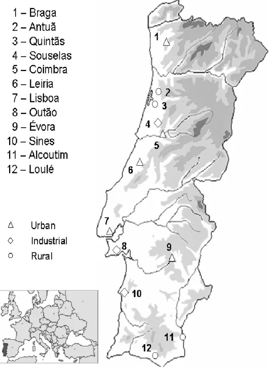
As shown in Figure 1, 12 sites in Portugal representing different land use were chosen to sample
Pinus pinea needles in one single campaign performed in 2006: Braga, Coimbra, Leiria, Lisboa and
Évora (urban); Souselas, Outão and Sines (industrial); and Antuã, Quintãs, Alcoutim and Loulé (rural). The needles, which had at least one year of exposure to the surrounding atmosphere, were collected whole from the lower branches of the trees and immediately wrapped in aluminium foil, sealed in plastic bags, frozen and kept protected from light until extraction.
2.5. Extraction and analysis of pine needles
The analytical methodology employed in the current study has been described previously (Araújo et al, 2012). In brief, five grams of needles (cut into 1 cm bits) were inserted in a glass tube, spiked with the internal standard (100 µg L-1) and extracted in a 360 W Selecta ultrasonic bath (J.P.
Selecta, Barcelona, Spain) for 10 minutes with 30 mL acetonitrile. This procedure was repeated three times, with fresh solvent. The sonicated extracts were combined and then reduced to about 0.5 mL in a rotary evaporator and purified following a clean-up procedure using 500 mg of ENVI 18 cartridges, conditioned with 5 mL of acetonitrile. The samples were then eluted with 50 mL of acetonitrile and the extracts reduced to 0.5 mL and transferred to 2-mL amber glass vials using dichloromethane. Finally, extracts were blown-down to dryness under a gentle nitrogen stream and reconstituted in 1 mL of acetonitrile.
Quantification was done by gas chromatography-mass spectrometry (GC/MS), using a Varian 3800 GC coupled with a Varian 4000 Ion Trap Mass Spectrometer (Lake Forest, CA, USA) injecting 1 µL of sample in splitless mode, under a helium (99.9999%) flow rate of 1.0 mL min-1.
The GC column was a FactorFour VF-5MS (30 m x 0.25 mm ID x 0.25 µm film thickness) also from Varian, and the temperature program started at 60 ºC (held for 1 min), then was raised at 50 ºC
10 min-1 to 160 ºC, at 2.5 ºC min-1 until 200 ºC, to 250 ºC at 50 ºC min-1, to 270 ºC at 2.5 ºC min-1 and
finally to 300 ºC at 50 ºC min-1. Acquisition was performed under in selected ion storage (SIS)
mode and the temperatures of the trap, transfer line and manifold were 200 ºC, 250 ºC and 50 ºC, respectively.
2.6. Quality assurance/quality control
The limits of detection (LODs, calculated by the signal-to-noise ratio) ranged from 0.13 to 5.56 ng g-1 (dry weight) for trifluralin and ametryn, respectively, in line with similar approaches applied
to related compounds (Martínez et al., 2004; Ratola et al., 2009). Good repeatability was obtained and the mean values for the intermediate precision were 13±10%. Recoveries found were between 50 and 105%, with a mean value of 72%, but the final results were not corrected accordingly, following the common procedure in biomonitoring studies when recoveries are not very low. Procedural blanks (only solvent spiked with the deuterated standards with no needles throughout the whole extraction/clean-up/analysis process) were done periodically, but the values for the concentration of the target compounds were below the LODs.
3. Results and discussion
The target pesticides chosen for this study cover a range of five chemical families (organophosphates, triazines, dinitroanilines, chloroacetamides, carbamates) and three main functions (herbicides, insecticides and acaricides), and were selected after a chemical scoring procedure.
3.1. Chemical scoring of pesticides
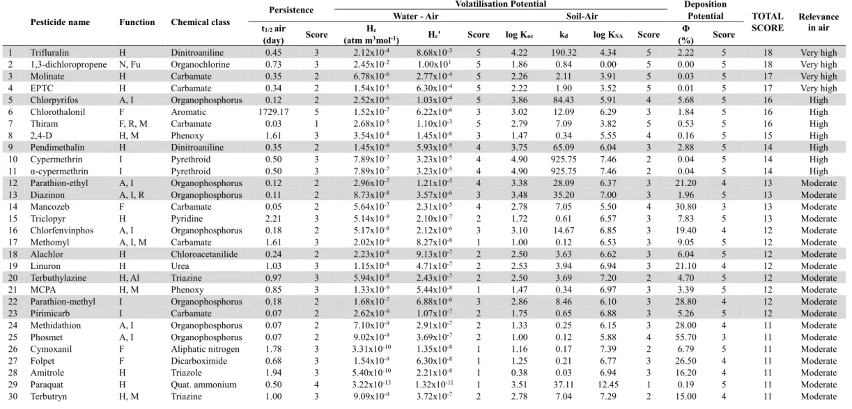
The objective of the chemical scoring was to classify a series of pesticides according to their ‘relevance’ in the atmosphere. A total of 70 pesticides were included in this prioritisation scheme (about 40% herbicides, 35% acaricides and insecticides and 25% fungicides), and the results can be
11 seen in Table 1. Overall, 4 pesticides were classified as of ‘Very high’ relevance in air, 7 as ‘High’, 31 as ‘Moderate’, 21 as ‘Low’ and 7 as ‘Very low’. The pesticides lacking the potential to reach/travel/remain in the air do not require a thorough monitoring in this compartment and, therefore, only those classified as ‘Very high’, ‘High’ or ‘Moderate’ are of main interest for the current study. However, due to the large number of compounds within this classification, only 18 pesticides were chosen to be monitored (cf. highlighted lines in Table 1), taking also into account the analytical limitations determined by the commercial standard mixtures available and the previous method validation in the research group (Araújo et al., 2012). This is why malathion, although ranked of ‘Low’ relevance in air, was also included in the monitoring scheme.
3.2. Levels and trends of pesticides in pine needles
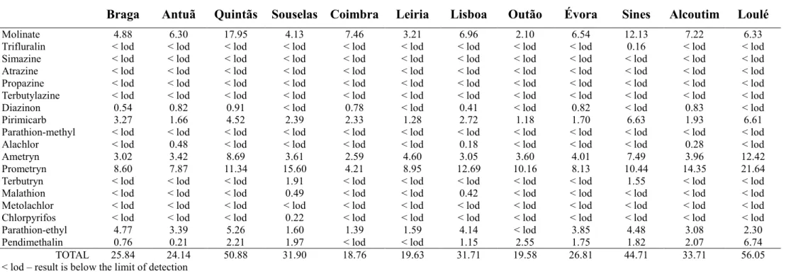
The levels of individual and total pesticides for the 12 sampling points chosen are shown in Table 2. Results indicate values of total pesticides between 18.8 ng g-1 (dw) in Coimbra, an urban area,
and 56.0 ng g-1 (dw) in Loulé, a rural site. Comparing to another typical SVOC pollution marker,
PAHs, these levels are an order of magnitude lower than those found for the same sites (Ratola et al., 2010). Several pesticides were not detected in any location. Individually, the compound with the highest mean concentrations was prometryn, with 11.2 ng g-1 (dw), with a sample maximum of 21.6
ng g-1 (dw) detected in Loulé. Molinate, ametryn and pirimicarb, followed, ranging from 3.0 to 7.1
ng g-1 (dw).
The information available in literature about levels of these pesticides in pine needles is almost inexistent. Still, it is interesting to realise that the detected levels of total pesticides follow the indicators of risk of phytopharmaceuticals use in Portugal by county (INE, 2009), where areas like Loulé or Quintãs present a high risk and cities like Braga, Coimbra and Leiria or rural areas like Antuã have a low use risk. While validating the analytical method used in this work, Araújo et al. (2012) analysed pine needles from four sites in the north of Portugal and concluded that the highest value of the total pesticides was found in Leixões, an important commercial port (45.89 ng g-1) and
12 current study. Individually, however, the trends presented some differences, with the most detected compound being ametryn (29.2%), followed by malathion (17.9%), molinate (16.4%) and prometryn (10.7%). In the other two similar studies found, Aston and Seiber (1996) reported higher concentration ranges than in the present work for diazinon (8-18 ng g-1, dw) and for chlorpyrifos
(14-30 ng g-1, dw) in P. ponderosa needles. Being these studies done in a different continent (North
America), it is plausible that the pesticides used can vary, given that also the crops can be different. The same authors also monitored simultaneously chlorpyrifos in air and pine needles (Aston and Seiber, 1997) and levels were 10-85 ng g-1 (dw) in pine needles and 0.12-180 ng m-3 in air.
Considerably more information on the levels of these pesticides in the nearby air would be needed to assess the degree of the respective correlations and further enhance the role of pine needles as biomonitors of the atmospheric load. Studies showing the incidence of the target pesticides in the atmosphere alone are more frequent, but still scarce. For instance, Yusà et al. (2009) reviewed the levels of several pesticides in the atmosphere from different countries and it can be seen that all of the target ones in the current study exist in the atmosphere, although not reflecting the incidence distribution found in the needles. The highest concentrations were found for malathion (4450 ng m-3), followed by diazinon (612 ng m-3) and pendimethalin (117 ng m-3). This may again be
explained by the different phytosanitary strategies followed by the countries involved. On another study performed in agricultural land in Canada, Yao et al. (2008) registered levels of diazinon, chlorpyrifos, trifluralin, metolachlor and atrazine up to 4370, 3.8, 1.6, 12.1 and 1.0 ng m-3,
respectively and confirmed as well the predominant presence of these pesticides in the atmospheric gas-phase. In a more global approach, Shunthirasingham et al. (2010) obtained a wide range of concentrations of trifluralin and pendimethalin in 29 sites worldwide and also differences even within the same continent. The highest levels were recorded in Paris (188 ng m-3) and Košetice,
Czech Republic (103 ng m-3), respectively. This may be due to the high using rates and frequencies
of these pesticides (Belden, 2012). As can be seen, the global distribution of these pesticides in the atmosphere is variable with the region of study.
13 Other types of pesticides have been reported in pine needles (such as HCB, HCHs, DDTs and chlordanes) their concentrations reached 76.1 ng g-1 for individual compounds, in this case lindane
(Hellström et al., 2004), yet remaining within the magnitudes shown in the present study.
Considering the pesticides in terms of chemical families, it can be seen (Figure 3, top left) that triazines predominate, followed by carbamates (both account to more than 80% of the total pesticides in each site). This can be the reflection of the pesticides sales in Portugal. In 2003, triazines and carbamates accounted for almost 60% of the total sales (Vieira, 2005), and only for OPPs is this correspondence not entirely verified. The incidence of these pesticides in the studies sites only reached a maximum of 20%, and their sales share in 2003 was of 37% (Vieira, 2005). Dinitroanilines and chloroacetamides show the lowest presence in the pine needle samples, usually fewer than 5%. It is important to note that the use of such pesticides in the 90s was quite intensive, and its use declined over the past few years due to severe restrictions imposed by the EU legislation. In fact, some pesticides have been banned and, therefore it is normal that the sales may have changed accordingly.
The trends by land occupation show that, in average, there is a predominance of the pesticides load in rural areas (41.2 ng g-1, dw), followed by industrial (32.1 ng g-1, dw) and urban ones (24.6
ng g-1, dw), as indicated in Figure 3 (top right). This is again in line with the indicators of risk of
phytopharmaceuticals use by county in Portugal, when it is clear that rural areas present the highest risks, and not so much in urban or industrial areas (INE, 2009). The chemical family patterns are, however, similar between site types, with only some differences seen for the urban sites, where the OPPs have the strongest percentage and dinitroanilines the lowest. (Figure 3, top right).
As to the target types of the pesticides, Figure 3 (bottom left) clearly shows the dominance of herbicides, with 65 to 95% of incidence in the sampling sites. This also reflects the sales trend, with herbicides having 83% of the combined total for herbicides, acaricides and insecticides in 2003 (Vieira, 2005). Furthermore, considering the pesticides sold by area of agricultural land, in 2007 herbicides accounted for 0.58 kg ha-1 and insecticides and acaricides with a total of 0.35 kg ha-1
14 the differences between site types are not profound. Still, acaricides have a stronger incidence in urban areas, which is admissible given the use of these pesticides in households for pest control. Herbicides, on the contrary, have the lowest urban presence, although the total incidence still shows a very high percentage (above 70%). The fact that the industrial sites studies are surrounded predominantly by rural areas instead of large urban settings is probably reflected in the clear similitude of industrial and rural trends in this case.
3.3. Risk of exposure
As mentioned before, the risk of exposure depends on the product of two factors: physicochemical properties that define the probability of the pesticide to occur in the air and their field presence as detected by the pine needles monitoring. As can be seen in Figure 4, maximum exposure risk results from the combination of a high chemical score and a high frequency of detection, while minimum risk is associated to the opposites, low chemical score and very low or no frequency of detection.
Figure 4 shows that molinate presents the highest risk of exposure. This is due to a very high chemical scoring (17) combined with a high frequency of occurrence, as it was detected in all analysed samples. In fact this was the pesticide with the second highest total and average concentration levels (85.2 ng g-1 and 7.1 ng g-1, respectively). On the other hand, trifluralin, also
with a very high chemical scoring (18), represents only a low risk as it was detected in only one sample and at the lowest concentration of all detected pesticides (0.16 ng g-1). The low occurrence
and concentration may be explained by its declining use, but also due to its extensive half-time in soil which reduces atmospheric emissions (Belden et al, 2012). Another explanation for this may be the fact that trifluralin undergoes direct photodegradation which reduces its occurrence in the atmosphere (Zeng and Arnold, 2013). Risk of exposure is therefore very limited. A similar behaviour was observed for chlorpyrifos and pendimethalin. Both have a high chemical score, but because of their different frequency of detection, their risk is low and high, respectively. Pesticides with moderate chemical score (10-13) show quite disperse behaviour. While parathion-ethyl,
15 pirimicarb, prometryn and ametryn show a high risk of exposure, due to their high frequency of occurrence, diazinon and alachlor present a moderate to low risk, which matches their occurrence in the pine needle samples. The same tendency is seen for their average concentrations. The other moderate chemical score pesticides were considered to be of a very low exposure risk, as they were not detected in any sample. Malathion and terbutryn show identical frequencies of occurrence, but due to their different chemical score (low and moderate, respectively), their exposure risk is distinctive, being very low for malathion and low for terburtyn. The same pattern can be verified for their average concentrations, as terbutryn shows levels nearly fourfold higher than malathion.
The main conclusion that can be drawn is that physicochemical properties of pollutants, even if combined through a chemical scoring methodology, are not enough to reflect thoroughly complex local phenomena that may occur and affect the levels of the target pollutants. Therefore, after most relevant pesticides to be monitored were chosen based on their probability of their atmospheric presence, the detected frequencies obtained by monitoring should be correlated with their respective chemical score in order to asses the effective risk of exposure to populations and environment. As opposed to active or passive air sampling, biomonitoring using pine needles exempt the need for a previous sampling site set-up and may act a “biological data loggers” of pollution as needles remain in the tree for several years.
3.4. Principal component analysis
The use of advanced multivariate statistics like principal component analysis (PCA) helps the analysis and interpretation of large multivariate data generated from environmental monitoring schemes (Terrado et al., 2006). This technique acts as a complement of classic univariate statistics and allows the unveiling of concealed environmental information (Navarro et al, 2006). In this case, Figure 5 shows that there is some separation in the scores plots between the site types, more visible in the plot of principal component (PC) 1 against PC 3 (Figure 5, bottom left) and particularly between the rural and the urban areas, which up to a point suggests different types of pesticides used in each case. In the loadings plot (Figure 5, bottom right), it can be seen that chloroacetamides,
16 triazines and dinitroanilines are more strongly linked to the rural areas, whereas OPPs have an affinity towards urban settings. These findings have some correspondence with the plot of PC 1 versus PC 2 (Figure 5, top right), except for OPPs, which seem in this case preferentially linked to rural sites. In this case, the information provided by the dataset is not entirely conclusive, which urges the establishment of further and more complete field campaigns to monitor these and other pesticides of interest.
3.5. Correlations with geo-energetic parameters
Trying to assess some more aspects of these pesticides behaviour, some correlations with geographic, meteorological and economical parameters were attempted using the Pearson test with several levels of significance. The results are displayed in Table 3. As can be seen, no significant correlations were found for the first ones, and only a few climatic trends, namely the total triazines with mean minimum, maximum and average temperatures and the sum of OPPs with total rainfall (p<0.10). The most significant correlations were with the mean average temperature, just like the positive trend with the total pesticides. This can be a reflection of a more extensive volatilisation of these compounds from the soils (in terms of target, the herbicides are those contributing to this relationship) into the atmosphere, favouring their entrapment by the waxy layer of pine needles. On the other hand, rainfall and temperature may have a significant importance on biotic and abiotic degradation and on the formation of non-extractable residues that influence persistence in soil and therefore reduces volatilisation (Loos et al., 2012). For the energetic consumption, more associations can be found, namely in indicators related to urban areas, such as domestic energy consumption or urban waste production. Dinitroanilines show the best correlations overall, and in terms of total pesticides, there are positive trends with agricultural energy consumption, water use and urban waste. This suggests that pesticides can be found virtually everywhere and their use is extended to the whole territory. It is interesting to notice that the sum of the insecticides correlates positively with non-domestic and industry energy consumption, which possibly denotes the incidence of their use in offices or industrial facilities.
17 Conclusions
The total concentration of 18 pesticides measured in pine needles from 12 sampling sites in Portugal ranged between 18.8 and 56.0 ng g-1 (dw). Triazines were the predominant chemical family,
followed by carbamates, whereas in terms of their target, herbicides clearly rule, with 65 to 95% of the total incidence. In general, the distribution of the pesticide families in urban, industrial and rural areas showed similarities, but there was some indication that the pesticides used in each of them could be different. Their risk of exposure was established based on chemical score and occurrence frequency. Molinate, a widely used pesticide in Portugal, offers the highest exposure risk, while terbutryn, parathion-methyl, metolachlor, atrazine, propazine and simazine show a very low risk, due to their absence in the analysed samples.
In terms of the relationships with geo-economical parameters, dinitroanilines show the best correlations and the total pesticides had a positive link with the mean average atmospheric temperature with geo-economical parameters, suggesting stronger volatilisation from soils into the atmosphere in the warmer sites. Overall it can be said that pine needles can act as reliable biomonitors of the pesticides in study, but more field campaigns are needed to be able to assess their behaviour more thoroughly.
Acknowledgements
The authors wish to thank Fundação para a Ciência e a Tecnologia (FCT - Portugal) for the Project PTDC/AGR-CFL/102597/2008 and grants SFRH/BPD/67088/2009 and SFRH/BPD/76974/2011. This work has been partially funded by the European Union Seventh Framework Programme-Marie Curie COFUND (FP7/2007-2013) under UMU Incoming Mobility Programme ACTion (U-IMPACT) Grant Agreement 267143. Dr. Olga Ferreira, is thanked for her collaboration in collecting the pine needle samples.
18 Amigo, J.M, Ratola, N., Alves A., 2011. Study of geographical trends of polycyclic aromatic
hydrocarbons using pine needles. Atmospheric Environment 45, 5988-5996.
Araújo, R., Ratola, N., Moreira, J.L., Santos, L., Alves A., 2012. Different extraction approaches for the biomonitoring of pesticides in pine needles. Environmental Technology 33, 2359-2363. Asman, W.A.H., Jorgensen, A., Bossi, R., Vejrup, K.V., Bugel Mogensen B., Glasius, M., 2005. Wet
deposition of pesticides and nitrophenols at two sites in Denmark: measurements and contributions from regional sources, Chemosphere 59, 1023-1031.
Aston L.S., Seiber, J.N., 1996. Methods for the comparative analysis of organophosphate residues in four compartments of needles of Pinus ponderosa, Journal of Agricultural and Food Chemistry 44, 2728-2735.
Aston L.S., Seiber, J.N., 1997. Fate of summertime airborne organophosphate pesticide residues in the Sierra Nevada mountains, Journal of Environmental Quality 26, 1483-1492.
Belden, J.B., Hanson, B.R., McMurry, S., Smith, L., Haukos D.A., 2012. Assessment of the effects of farming and conservation programs on pesticide deposition in high plain wetlands.
Environmental Science and Technology 46, 3424-3432.
Bidleman, T.F., 1999. Atmospheric transport and air-surface exchange of pesticides, Water Air and Soil Pollution 115, 115-166.
Boethling, R.S., Howard, P.H., Meylan, W.M., 2004. Finding and estimating chemical property data for environmental assessment. Environmental Toxicology and Chemistry 23, 2290-2308. Breivik, K., Alcock, R., Li, Y.F., Bailey, R.E., Fiedler H., Pacyna, J.M., 2004. Primary sources of
selected POPs: regional and global scale emission inventories, Environmental Pollution 128, 3-16.
Chaplain, V., Mamy, L., Vieublé-Gonod, L., Mougin, C., Benoit, P., Barriuso, E., Nélieu, S., 2011. Fate of Pesticides in Soils: Toward an Integrated Approach of Influential Factors, Pesticides in the Modern World - Risks and Benefits,
http://www.intechopen.com/books/pesticides-in-the-modern-world-risks-and-benefits/fate-of-pesticides-in-soils-toward-an-integrated-approach-of-influential-factors (accessed December
2012)
Coscollà, C., Colin, P., Yahyaoui, A., Petrique, O., Yusà, V., Mellouki, A., Pastor, A. 2010. Occurrence of currently used pesticides in ambient air of Centre Region (France), Atmospheric Environment 44, 3915-3925.
Davie-Martin, C.L., Hageman, K.J., Chin, Y.-P., 2013. An improved screening tool for predicting volatilisation of pesticides applied to soils. Environmental Science and Technology 47,
19 8868-8876.
Dolinova, J., Klánová, J., Klan, P., Holoubek, I., 2004. Photodegradation of organic pollutants on the spruce needle wax surface under laboratory conditions. Chemosphere 57, 1399–1407. Environmental Protection Agency (EPA), 2011. Estimation Program Interface (EPI) Suite, version
4.11. http://www.epa.gov/opptintr/exposure/pubs/episuitedl.htm (accessed February 2013) European Union Pesticide Database (EUPD), 2013.
http://ec.europa.eu/sanco_pesticides/public/index.cfm?event=activesubstance.selection&a=1 (accessed February 2013)
Grimalt, J., van Drooge, B.L., 2006. Polychlorinated biphenyls in mountain pine (Pinus uncinata) needles from Central Pyrenean high mountains (Catalonia, Spain). Ecotoxicology and Environmental Safety 63, 61-67.
Guth, J.A., Reischmann, F.J., Allen, R., Arnold, D., Hassink, J., Leake, C.R., Skidmore, M.W., Reeves, G.L., 2004. Volatilisation of crop protection chemicals from crop and soil surfaces under controlled conditions – prediction of volatile losses from physic-chemical properties. Chemosphere 57, 871-887.
Harner, T., Bidleman, T.F., 1998. Octanol−air partition coefficient for describing particle/gas partitioning of aromatic compounds in urban air. Environmental Science and Technology 32, 1494-1502.
Hellström, A., Kylin, H., Strachan, W.M.J., Jensen, S., 2004. Distribution of some organochlorine compounds in pine needles from Central and Northern Europe. Environmental Pollution 128, 29-48.
Hellström, A., Kylin, H., Strachan, W.M.J., Jensen, S., 2004. Distribution of some organochlorine compounds in pine needles from Central and Northern Europe. Environmental Pollution 128, 29-48.
INE (Instituto Nacional de Estatística – Statistics Portugal), 2009. Indicadores Agro-Ambientais 1989-2007. ISBN 978-989-25-0041-6, Lisboa, Portugal, 175 pp.
INE (Instituto Nacional de Estatística – Statistics Portugal), 2013. www.ine.pt (assessed October 2013).
Institute for Environment and Health (IEH), 2004. A Screening Method for Ranking Chemicals by their Fate and Behaviour in the Environment and Potential Toxic Effects in Humans
Following Non-occupational Exposure (Web Report W14). Leicester, UK. http://www.le.ac.uk/ieh/ (accessed June 2013).
Juraske, R., Antón, A., Castell, F., Huijbregts, M.A.J., 2007. PestScreen: A screening approach for scoring and ranking pesticides by their environmental and toxicological concern.
20 Environment International 33, 886-893.
Klánová, J., Čupr, P., Baráková, D., Šeda, Z., Anděl, P., Holoubek, I., 2009. Can pine needles indicate trends in the air pollution levels at remote sites? Environmental Pollution 157, 3248-3254.
Köck-Schulmeier, M., Ginebreda, A., Postigo, C., Garrido, T., Fraile, J., Alda, M.L., Barceló, D. 2014. Four-year advanced monitoring program of polar pesticides in groundwater of Catalonia (NE-Spain). Science of the Total Environment 470-471, 1087-1089.
Krieger, R.I., Handbook of pesticide toxicology, Volume 1. 2001. Academic Press, San Diego, USA. Lamprea, K., Ruban, V., 2011. Characterization of atmospheric deposition and runoff water in a
small suburban catchment, Environment Technology 32, 1141-1149.
Loos, M., Krauss, M., Fenner, K., 2012. Pesticide nonextractable residue formation in soil: Insights from inverse modeling of degradation time series. Environmental Science and Technology 46, 9830-9837.
Marcomini, A., Perin, G., Stelluto, S., Da Ponte, M., Traverso, P., 1991. Selected herbicides in treated and untreated surface water, Environment Technology 12, 1127-1135.
Martinez, E., Gros, M., Lacorte S., Barceló, D., 2004. Simplified procedures for the analysis of polycyclic aromatic hydrocarbons in water, sediments and mussels. Journal of
Chromatography A 1047, 181-188.
Navarro, A., Tauler, R., Lacorte, S., Barceló, D., 2006. Chemometrical investigation of the presence and distribution of organochlorine and polyaromatic compounds in sediments of the Ebro River Basin. Analytical and Bioanalytical Chemistry 385, 1020-1030.
Piccardo, M.T., Pala, M., Bonaccurso, B., Stella, A., Redaelli, A., Paola G., Valério F., 2005. Pinus
nigra and Pinus pinaster needles as passive samplers of polycyclic aromatic hydrocarbons.
Environmental Pollution 133, 293-301.
Portuguese National Authority for Animal Health, Phytosanitation and Food, 2013. PAN - Projeto de plano de ação nacional para o uso sustentável dos produtos fitofarmacêuticos – Contexto nacional da utilização de produtos fitofarmacêuticos.Volume II.
https://www.google.pt/url?sa=t&rct=j&q=&esrc=s&source=web&cd=1&ved=0CC0QFjAA& url=http%3A%2F%2Fwww.dgv.min-agricultura.pt%2Fxeov21%2Fattachfileu.jsp%3Flook_p arentBoui%3D6321372%26att_display%3Dn%26att_download%3Dy&ei=euKNUoydJ6iJ7A bH2YH4DQ&usg=AFQjCNFSqtVD-Sgx-TbgjMbj71LMxlIeIA&bvm=bv.56987063,bs.1,d.Y ms (accessed March 2013)
21 Portugal: Biomonitoring with Pinus pinea and Pinus pinaster Needles. Archives of
Environmental Contamination and Toxicology 58, 631-647.
Ratola, N., Lacorte, S., Alves A., Barceló, D., 2006. Analysis of polycyclic aromatic hydrocarbons in pine needles by gas chromatography–mass spectrometry Comparison of different
extraction and clean-up procedures, Journal of Chromatography A 1114, 198-204. Ratola, N., Santos, L., Alves, A., Lacorte, S., 2011. Pine needles as passive bio-samplers to
determine polybrominated diphenyl ethers. Chemosphere 85, 247-252.
Rusco, E., Jones, R., Bidoglio, G., 2001. Organic Matter in the soils of Europe: Present status and future trends. European Commission Directorate General JRC, Joint Research Centre, Institute for Environment and Sustainability, European Soil Bureau
Sarigiannis, D.A., Kontoroupis, P., Solomou, E.S., Nikolaki, S., Karabelas, A.J. 2013. Inventory of pesticide emissions into the air in Europe. Atmospheric Environment 75, 6-14.
Shunthirasingham, C., Oyiliagu, C.E., Cao, X., Gouin, T., Wania, F., Lee, S.-C., Pozo, K., Harner, T., Muir, D.C.G.., 2010. Spatial and temporal pattern of pesticides in the global atmosphere. Journal of Environmental Monitoring 12, 1650–1657.
Snyder, E.M., Snyder, S.A., Giesy, J.P., Blonde, A.A., Hurlburt, G.K., Summer, C.L., Mitchell, R.R., Bush, D., 2000. SCRAM: A scoring and ranking system for persistent, bioaccumulative, and toxic substances for the North American great lakes. Environmental Science and Pollution Research 7, 219-224.
Stangroom, S.J., Lester J.N., Collins, C.D., 2000. Abiotic behaviour of organic micropollutants in soils and the aquatic environment. A review: I. Partitioning, Environment Technology 21, 845-863.
Terrado, M., Barceló, D., Tauler, R., 2006. Identification and distribution of contamination sources in the Ebro river basin by chemometrics modelling coupled to geographical information systems. Talanta 70, 691–704.
Tremolada, P., Burnett, V., Calamari, D., Jones, K.C., 1996. Spatial distribution of PAHs in the U.K. atmosphere using pine needles. Environmental Science and Technology 30, 3570-3477. van der Werf, H.M.G.., 1996. Assessing the impact of pesticides on the environment. Agriculture,
Ecosystems and Environment 60, 81–96.
Vieira, M.M., 2005. Vendas de produtos fitofarmacêuticos em Portugal em 2003. Direcção Geral de Protecção das Culturas – Direcção de Serviços de Produtos Fitofarmacêuticos.
PPA(AB)-01/05.
22 Agrárias 35, 11-22. (in Portuguese)
Xu, D., Zhong, W., Deng, L., Chai, Z., Mao, X., 2004. Regional distribution of organochlorinated pesticides in pine needles and its indication for socioeconomic development. Chemosphere 54, 743-752.
Yao, Y., Harner, T., Blanchard, P., Tuduri, L., Waite, D., Poissant, L., Murphy, C., Belzer, W., Aulagnier, F., Sverko, E., 2008. Pesticides in the atmosphere across Canadian agricultural regions. Environmental Science and Technology 42, 5931–5937.
Yusà, V., Coscollà, C., Mellouki, W., Pastor A., de la Guardia, M., 2009. Sampling and analysis of pesticides in ambient air. Journal of Chromatography A 1216, 2972-2983.
Zeng, T., Arnold, W.A., 2013. Pesticide Photolysis in Prairie Potholes: Probing Photosensitized Processes. Environmental Science and Technology 47, 6735-6745.
23 List of Tables
Table 1 – Overall rating of pesticides in the prioritization scheme for monitoring in the air compartment.
Pesticide name Function Chemical class
Persistence Volatilisation Potential Deposition
Potential TOTAL SCORE
Relevance in air
Water - Air Soil-Air
t1/2 air
(day) Score
Hc
(atm m3mol-1) Hc' Score log Koc kd log KSA Score
Φ
(%) Score
1 Trifluralin H Dinitroaniline 0.45 3 2.12x10⁻⁴ 8.68x10⁻³ 5 4.22 190.32 4.34 5 2.22 5 18 Very high
2 1,3-dichloropropene N, Fu Organochlorine 0.73 3 2.45x10⁻² 1.00x101 5 1.86 0.84 0.00 5 0.00 5 18 Very high
3 Molinate H Carbamate 0.35 2 6.78x10⁻⁶ 2.77x10⁻⁴ 5 2.26 2.11 3.91 5 0.03 5 17 Very high
4 EPTC H Carbamate 0.34 2 1.54x10⁻⁵ 6.30x10⁻⁴ 5 2.22 1.90 3.52 5 0.01 5 17 Very high
5 Chlorpyrifos A, I Organophosphorus 0.12 2 2.52x10⁻⁶ 1.03x10⁻⁴ 5 3.86 84.43 5.91 4 5.68 5 16 High
6 Chlorothalonil F Aromatic 1729.17 5 1.52x10⁻⁷ 6.22x10⁻⁶ 3 3.02 12.09 6.29 3 1.84 5 16 High
7 Thiram F, R, M Carbamate 0.03 1 2.68x10⁻⁵ 1.10x10⁻³ 5 2.79 7.09 3.82 5 0.53 5 16 High
8 2,4-D H, M Phenoxy 1.61 3 3.54x10⁻⁸ 1.45x10⁻⁶ 3 1.47 0.34 5.55 4 0.16 5 15 High
9 Pendimethalin H Dinitroaniline 0.35 2 1.45x10⁻⁶ 5.93x10⁻⁵ 4 3.75 65.09 6.04 3 2.88 5 14 High
10 Cypermethrin I Pyrethroid 0.50 3 7.89x10⁻⁷ 3.23x10⁻⁵ 4 4.90 925.75 7.46 2 0.04 5 14 High
11 α-cypermethrin I Pyrethroid 0.50 3 7.89x10⁻⁷ 3.23x10⁻⁵ 4 4.90 925.75 7.46 2 0.04 5 14 High
12 Parathion-ethyl A, I Organophosphorus 0.12 2 2.96x10⁻⁷ 1.21x10⁻⁵ 4 3.38 28.09 6.37 3 21.20 4 13 Moderate
13 Diazinon A, I, R Organophosphorus 0.11 2 8.73x10⁻⁸ 3.57x10⁻⁶ 3 3.48 35.20 7.00 3 1.96 5 13 Moderate
14 Mancozeb F Carbamate 0.05 2 5.64x10⁻⁷ 2.31x10⁻⁵ 4 2.78 7.05 5.50 4 30.80 3 13 Moderate
15 Triclopyr H Pyridine 2.21 3 5.14x10⁻⁹ 2.10x10⁻⁷ 2 1.72 0.61 6.57 3 7.83 5 13 Moderate
16 Chlorfenvinphos A, I Organophosphorus 0.18 2 5.17x10⁻⁸ 2.12x10⁻⁶ 3 3.10 14.67 6.85 3 19.40 4 12 Moderate
17 Methomyl A, I, M Carbamate 1.61 3 2.02x10⁻⁹ 8.27x10⁻⁸ 1 1.00 0.12 6.53 3 9.05 5 12 Moderate
18 Alachlor H Chloroacetanilide 0.24 2 2.23x10⁻⁸ 9.13x10⁻⁷ 2 2.50 3.63 6.62 3 6.04 5 12 Moderate
19 Linuron H Urea 1.03 3 1.15x10⁻⁸ 4.71x10⁻⁷ 2 2.53 3.94 6.94 3 21.10 4 12 Moderate
20 Terbuthylazine H, Al Triazine 0.97 3 5.94x10⁻⁹ 2.43x10⁻⁷ 2 2.50 3.69 7.20 2 4.70 5 12 Moderate
21 MCPA H, M Phenoxy 0.85 3 1.33x10⁻⁹ 5.44x10⁻⁸ 1 1.47 0.34 6.97 3 3.39 5 12 Moderate
22 Parathion-methyl I Organophosphorus 0.18 2 1.68x10⁻⁷ 6.88x10⁻⁶ 3 2.86 8.46 6.10 3 28.80 4 12 Moderate
23 Pirimicarb I Carbamate 0.07 2 2.62x10⁻⁹ 1.07x10⁻⁷ 2 1.75 0.65 6.88 3 5.26 5 12 Moderate
24 Methidathion A, I Organophosphorus 0.07 2 7.10x10⁻⁹ 2.91x10⁻⁷ 2 1.33 0.25 6.15 3 28.00 4 11 Moderate
25 Phosmet A, I Organophosphorus 0.07 2 9.02x10⁻⁹ 3.69x10⁻⁷ 2 1.00 0.12 5.88 4 55.70 3 11 Moderate
26 Cymoxanil F Aliphatic nitrogen 1.78 3 3.31x10⁻¹⁰ 1.35x10⁻⁸ 1 1.16 0.17 7.39 2 6.79 5 11 Moderate
27 Folpet F Dicarboximide 0.68 3 1.54x10⁻⁹ 6.30x10⁻⁸ 1 1.25 0.21 6.77 3 26.50 4 11 Moderate
28 Amitrole H Triazole 1.94 3 5.40x10⁻¹⁰ 2.21x10⁻⁸ 1 0.38 0.03 6.94 3 16.20 4 11 Moderate
29 Paraquat H Quat. ammonium 0.50 4 3.22x10⁻¹³ 1.32x10⁻¹¹ 1 3.51 37.11 12.45 1 0.19 5 11 Moderate
24 31 Carbaryl I Carbamate 0.41 2 3.14x10⁻⁹ 1.28x10⁻⁷ 2 2.55 4.12 7.52 2 7.93 5 11 Moderate
32 Endosulfan A, I Organochlorine 1.30 3 9.03x10⁻⁸ 3.70x10⁻⁶ 3 3.83 78.43 7.33 1 32.10 3 10 Moderate
33 Carbofuran A, I, N, M Carbamate 0.41 2 1.63x10⁻⁹ 6.67x10⁻⁸ 1 1.98 1.11 7.28 2 0.17 5 10 Moderate
34 Metalaxyl F Amide 0.40 2 8.05x10⁻¹⁰ 3.29x10⁻⁸ 1 1.59 0.45 7.27 2 6.77 5 10 Moderate
35 Ametryn H Triazine 0.38 2 6.85x10⁻⁹ 2.80x10⁻⁷ 2 2.63 4.97 7.26 2 13.50 4 10 Moderate
Table 1 – Overall rating of pesticides in the prioritization scheme for monitoring in the air compartment (cont.).
Pesticide name Function Chemical class
Persistence Volatilisation Potential Deposition Potential
TOTAL SCORE
Relevance in air
Water - Air Soil-Air
t1/2 air
(day) Score
Hc
(atm m3mol-1) Hc' Score log Koc kd log KSA Score
Φ
(%) Score
36 Atrazine H Triazine 0.39 2 4.47x10⁻⁹ 1.83x10⁻⁷ 2 2.35 2.60 7.18 2 17.60 4 10 Moderate
37 Metolachlor H Chloroacetanilide 0.19 2 1.49x10⁻⁹ 6.10x10⁻⁸ 1 2.69 5.67 7.98 2 5.42 5 10 Moderate
38 Prometryn H Triazine 0.28 2 9.09x10⁻⁹ 3.72x10⁻⁷ 2 2.82 7.61 7.32 2 14.60 4 10 Moderate
39 Propanil H Amide 2.83 3 4.50x10⁻⁹ 1.84x10⁻⁷ 2 2.25 2.04 7.08 2 30.10 3 10 Moderate
40 Propazine H Triazine 0.29 2 5.94x10⁻⁹ 2.43x10⁻⁷ 2 2.54 3.99 7.23 2 16.00 4 10 Moderate
41 Simazine H Triazine 0.97 3 3.37x10⁻⁹ 1.38x10⁻⁷ 2 2.17 1.70 7.13 2 45.60 3 10 Moderate
42 Bromoxynil H, M Nitrile 50.83 5 8.60x10⁻¹⁰ 3.52x10⁻⁸ 1 2.52 3.83 8.06 1 47.10 3 10 Moderate
43 Tetradifon A Bridged diphenyl 30.25 4 2.32x10⁻⁸ 9.49x10⁻⁷ 2 4.23 196.11 8.32 2 99.80 1 9 Low
44 Amitraz A, I Formamidine 0.08 2 1.48x10⁻⁸ 6.06x10⁻⁷ 2 5.41 2981.9 9.69 1 18.30 4 9 Low
45 Azinphos-methyl A, I Organophosphorus 0.07 2 2.86x10⁻¹⁰ 1.17x10⁻⁸ 1 1.72 0.60 7.82 2 27.40 4 9 Low
46 Dimethoate A, I, M Organophosphorus 0.14 2 2.11x10⁻¹¹ 8.63x10⁻¹⁰ 1 1.11 0.15 8.56 1 4.92 5 9 Low
47 Benalaxyl F Amide 0.39 2 7.84x10⁻¹⁰ 3.21x10⁻⁸ 1 3.51 37.54 9.07 1 5.00 5 9 Low
48 Ofurace F Amide 0.46 3 1.51x10⁻⁹ 6.18x10⁻⁸ 1 2.26 2.12 7.57 2 43.60 3 9 Low
49 Propamocarb F Carbamate 0.11 2 1.34x10⁻¹⁰ 5.48x10⁻⁹ 1 2.00 1.17 8.39 1 0.00 5 9 Low
50 Ziram F, R Carbamate 0.08 2 1.74x10⁻⁹ 7.12x10⁻⁸ 1 3.05 12.93 8.26 1 7.63 5 9 Low
51 Chloridazon H Pyrazole 0.26 2 6.54x10⁻¹² 2.68x10⁻¹⁰ 1 2.59 4.50 10.24 1 6.23 5 9 Low
52 Diuron H Urea 0.98 3 5.33x10⁻¹⁰ 2.18x10⁻⁸ 1 2.04 1.27 7.82 2 55.70 3 9 Low
53 Metribuzin H Triazinone 0.59 3 1.81x10⁻¹² 7.41x10⁻¹¹ 1 1.73 0.62 10.02 1 29.30 4 9 Low
54 Acephate I Organophosphorus 0.96 3 2.81x10⁻¹² 1.15x10⁻¹⁰ 1 1.00 0.12 9.39 1 20.10 4 9 Low
55 Dicofol A Bridged diphenyl 3.12 3 5.59x10⁻¹⁰ 2.29x10⁻⁸ 1 4.10 147.06 9.81 1 57.70 3 8 Low
56 Azinphos-ethyl A, I Organophosphorus 0.06 2 5.04x10⁻¹⁰ 2.06x10⁻⁸ 1 2.24 2.00 8.02 1 28.40 4 8 Low
57 Malathion A, I Organophosphorus 0.14 2 8.39x10⁻¹⁰ 3.43x10⁻⁸ 1 1.50 0.36 7.19 2 34.70 3 8 Low
58 Fenarimol F Pyrimidine 2.72 3 4.21x10⁻¹³ 1.72x10⁻¹¹ 1 4.22 193.42 13.05 1 49.00 3 8 Low
59 Captan F, B Dicarboximide 0.04 1 4.59x10⁻⁹ 1.88x10⁻⁷ 2 2.40 2.93 7.22 2 38.10 3 8 Low
60 Isoproturon H Urea 0.89 3 1.89x10⁻⁹ 7.73x10⁻⁸ 1 2.30 2.31 7.51 2 77.90 2 8 Low
61 Deltamethrin I, M Pyrethroid 0.45 3 6.06x10⁻⁸ 2.48x10⁻⁶ 3 4.90 925.75 8.57 1 95.60 1 8 Low
62 Dodine F Aliphatic nitrogen 0.10 2 6.02x10⁻¹⁹ 2.46x10⁻¹⁷ 1 3.40 28.81 18.07 1 48.90 3 7 Low
63 Chlortoluron H Urea 0.27 2 7.94x10⁻¹⁰ 3.25x10⁻⁸ 1 2.04 1.27 7.64 2 75.20 2 7 Low
25 65 Carbendazim F, M Carbamate 0.05 2 1.49x10⁻¹² 6.10x10⁻¹¹ 1 2.58 4.45 10.88 1 82.10 2 6 Very low
66 Glyphosate H Organophosphorus 0.14 2 4.08x10⁻¹⁹ 1.67x10⁻¹⁷ 1 0.00 0.01 16.03 1 87.10 2 6 Very low
67 Metamitron H Triazinone 0.55 3 5.85x10⁻¹² 2.39x10⁻¹⁰ 1 2.15 1.65 9.88 1 91.70 1 6 Very low
68 Tebuconazole F Triazole 0.93 3 5.18x10⁻¹⁰ 2.12x10⁻⁸ 1 3.19 17.8 8.93 1 96 1 6 Very low
69 Benomyl F, Mi Benzimidazole 0.05 2 1.23x10⁻¹² 5.03x10⁻¹¹ 1 2.53 3.90 10.91 1 97.30 1 5 Very low
70 Dimethomorph F Morpholine 0.03 1 1.01x10⁻¹⁵ 4.13x10⁻¹⁴ 1 3.76 66 15.2 1 93.7 1 4 Very low A – acaricide, Al – algericide, B – bactericide, F – fungicide, Fu – fumigant, H – herbicide, I – insecticide, M – metabolite, Mi – miticide, N – nematicide, R – repellent
Table 2. Concentrations of individual and total target pesticides for the 12 sampling sites considered (in ng g-1, dry weight).
Braga Antuã Quintãs Souselas Coimbra Leiria Lisboa Outão Évora Sines Alcoutim Loulé
Molinate 4.88 6.30 17.95 4.13 7.46 3.21 6.96 2.10 6.54 12.13 7.22 6.33
Trifluralin < lod < lod < lod < lod < lod < lod < lod < lod < lod 0.16 < lod < lod
Simazine < lod < lod < lod < lod < lod < lod < lod < lod < lod < lod < lod < lod
Atrazine < lod < lod < lod < lod < lod < lod < lod < lod < lod < lod < lod < lod
Propazine < lod < lod < lod < lod < lod < lod < lod < lod < lod < lod < lod < lod
Terbutylazine < lod < lod < lod < lod < lod < lod < lod < lod < lod < lod < lod < lod
Diazinon 0.54 0.82 0.91 < lod 0.78 < lod 0.41 < lod 0.82 < lod 0.83 < lod
Pirimicarb 3.27 1.66 4.52 2.39 2.33 1.28 2.72 1.18 1.70 6.63 1.93 6.61
Parathion-methyl < lod < lod < lod < lod < lod < lod < lod < lod < lod < lod < lod < lod
Alachlor < lod 0.48 < lod < lod < lod < lod 0.18 < lod < lod < lod 0.28 < lod
Ametryn 3.02 3.42 8.69 3.61 2.59 4.60 3.05 3.60 4.01 7.49 3.96 12.42
Prometryn 8.60 7.87 11.34 15.60 4.21 8.95 12.69 10.16 8.13 10.44 14.35 21.64
Terbutryn < lod < lod < lod 1.91 < lod < lod < lod < lod < lod 1.55 < lod < lod
Malathion < lod < lod < lod 0.49 < lod < lod 0.42 < lod < lod < lod < lod < lod
Metolachlor < lod < lod < lod < lod < lod < lod < lod < lod < lod < lod < lod < lod
Chlorpyrifos < lod < lod < lod 0.22 < lod < lod < lod < lod < lod < lod < lod < lod
Parathion-ethyl 4.77 3.39 5.26 1.60 1.39 1.59 4.14 < lod 3.85 4.48 3.08 2.30
Pendimethalin 0.76 0.21 2.21 1.97 < lod < lod 1.15 2.55 1.75 1.82 2.07 6.74
TOTAL 25.84 24.14 50.88 31.90 18.76 19.63 31.71 19.58 26.81 44.71 33.71 56.05
< lod – result is below the limit of detection
Table 3. Pearson test (n=12) for the correlations between chemical families and functions of pesticides and socio-economic and meteorological parameters.
26
PARAMETERS Total Ps SUM Carb SUM Triaz SUM CAAs SUM DNAs SUM OPPs SUM Herb SUM Acar SUM Ins
Population (hab) -0,1042 -0,0781 -0,1463 0,1347 -0,1974 0,2712 p < 0.10 -0,1587 0,2712 -0,0836
Density (hab/km2) -0,1551 -0,0822 -0,2065 0,1241 -0,2319 0,2007 p < 0.05 -0,1969 0,2007 -0,1439
Elevation (m) -0,1740 -0,1412 -0,2694 -0,1255 -0,0853 0,3698 p < 0.01 -0,2527 0,3698 -0,1271
Burnt area (ha) -0,1924 -0,1442 -0,2605 -0,1973 -0,1933 0,3317 -0,2915 0,3317 -0,0033
Total Rainfall (mm) -0,1332 0,1305 -0,3535 0,2314 -0,4920 0,5141 -0,2469 0,5141 -0,0294
Total wind speed (m/s) 0,0339 0,1145 -0,1160 0,0660 -0,0321 0,3544 -0,0177 0,3544 -0,0202
Mean min temp (ºC) 0,4885 0,2572 0,5219 0,1580 0,4233 0,1274 0,5274 0,1274 0,2317
Mean avg temp (ºC) 0,6148 0,3725 0,6584 0,0971 0,5196 0,0257 0,6550 0,0257 0,4655
Mean max temp (ºC) 0,4142 0,1295 0,5443 0,0772 0,4702 -0,1182 0,4761 -0,1182 0,2549
PER CAPITA
Autom. Fuel cons. (tep) -0,0514 -0,0133 -0,0054 0,0503 -0,1603 -0,1370 -0,0922 -0,1370 0,2885
Diesel (%) 0,1158 -0,0080 0,1568 0,6513 0,0605 0,1014 0,1533 0,1014 -0,1642
Electric (Domestic, kWh) 0,4881 0,0649 0,6954 -0,3270 0,7781 -0,2653 0,5508 -0,2653 0,4745
Electric (Non domestic, kWh) 0,4558 0,4781 0,3317 -0,2128 0,2289 0,1822 0,3897 0,1822 0,7048
Electric (Industry, kWh) 0,2813 0,4528 0,1123 -0,1704 0,0311 0,0974 0,2199 0,0974 0,5593
Electric (Agriculture, kWh) 0,5731 0,6071 0,3780 -0,2469 0,3563 0,2908 0,5874 0,2908 0,3058
Total water (m3) 0,5528 0,2133 0,6772 -0,3318 0,7180 -0,1455 0,5753 -0,1455 0,6509
Urban waste (t) 0,6160 0,3524 0,6584 -0,5152 0,7353 -0,0664 0,6329 -0,0664 0,6785
27 Figure Captions
28 Figure 2. Profile assessment criteria and scoring scheme.
29 Figure 3. Incidence of pesticides by chemical family (top) and main function (bottom) for all sampling sites (left) and according to land occupation (right).
30 Figure 4. Risk of exposure chart.
Legend:
Very low 0.0 – 1.4 Low 1.4 – 4.2 Moderate 4.2 – 8.2 High 8.2 - 13.4 Very high 13.4 – 20.0
Chemical score 0% 5% 10% 15% 20% 25% 30% 35% 40% 45% 50% 55% 60% 65% 70% 75% 80% 85% 90% 95% 100% Frequency of occurrence Very High 20 0.0 1.0 2.0 3.0 4.0 5.0 6.0 7.0 8.0 9.0 10.0 11.0 12.0 13.0 14.0 15.0 16.0 17.0 18.0 19.0 20.0 19 0.0 1.0 1.9 2.9 3.8 4.8 5.7 6.7 7.6 8.6 9.5 10.5 11.4 12.4 13.3 14.3 15.2 16.2 17.1 18.1 19.0 18 0.0 0.9 TFL 2.7 3.6 4.5 5.4 6.3 7.2 8.1 9.0 9.9 10.8 11.7 12.6 13.5 14.4 15.3 16.2 17.1 18.0 17 0.0 0.9 1.7 2.6 3.4 4.3 5.1 6.0 6.8 7.7 8.5 9.4 10.2 11.1 11.9 12.8 13.6 14.5 15.3 16.2 MOL High 16 0.0 0.8 CPF 2.4 3.2 4.0 4.8 5.6 6.4 7.2 8.0 8.8 9.6 10.4 11.2 12.0 12.8 13.6 14.4 15.2 16.0 15 0.0 0.8 1.5 2.3 3.0 3.8 4.5 5.3 6.0 6.8 7.5 8.3 9.0 9.8 10.5 11.3 12.0 12.8 13.5 14.3 15.0 14 0.0 0.7 1.4 2.1 2.8 3.5 4.2 4.9 5.6 6.3 7.0 7.7 8.4 9.1 9.8 10.5 11.2 PDM 12.6 13.3 14.0 Moderate 13 0.0 0.7 1.3 2.0 2.6 3.3 3.9 4.6 5.2 5.9 6.5 7.2 DZN 8.5 9.1 9.8 10.4 11.1 EP 12.4 13.0
12 MEP TBA 0.6 1.2 1.8 2.4 ALA 3.6 4.2 4.8 5.4 6.0 6.6 7.2 7.8 8.4 9.0 9.6 10.2 10.8 11.4 PIR
11 0.0 0.6 1.1 TBT 2.2 2.8 3.3 3.9 4.4 5.0 5.5 6.1 6.6 7.2 7.7 8.3 8.8 9.4 9.9 10.5 11.0 10 MLC ATR PRZ SIZ 0.5 1.0 1.5 2.0 2.5 3.0 3.5 4.0 4.5 5.0 5.5 6.0 6.5 7.0 7.5 8.0 8.5 9.0 9.5 AME PRO Low 9 0.0 0.5 0.9 1.4 1.8 2.3 2.7 3.2 3.6 4.1 4.5 5.0 5.4 5.9 6.3 6.8 7.2 7.7 8.1 8.6 9.0 8 0.0 0.4 0.8 MLT 1.6 2.0 2.4 2.8 3.2 3.6 4.0 4.4 4.8 5.2 5.6 6.0 6.4 6.8 7.2 7.6 8.0 7 0.0 0.4 0.7 1.1 1.4 1.8 2.1 2.5 2.8 3.2 3.5 3.9 4.2 4.6 4.9 5.3 5.6 6.0 6.3 6.7 7.0 Very low 6 0.0 0.3 0.6 0.9 1.2 1.5 1.8 2.1 2.4 2.7 3.0 3.3 3.6 3.9 4.2 4.5 4.8 5.1 5.4 5.7 6.0 5 0.0 0.3 0.5 0.8 1.0 1.3 1.5 1.8 2.0 2.3 2.5 2.8 3.0 3.3 3.5 3.8 4.0 4.3 4.5 4.8 5.0 4 0.0 0.2 0.4 0.6 0.8 1.0 1.2 1.4 1.6 1.8 2.0 2.2 2.4 2.6 2.8 3.0 3.2 3.4 3.6 3.8 4.0
TBA – Terbutylazine, MEP - Parathion-methyl, MLC – Metolachlor, ATR – Atrazine, PRZ – Propazine, SIZ – Simazine, TFL – Trifluralin, CPF - Chlorpyrifos, TBT – Terbutryn, MLT – Malathion, ALA – Alachlor, DZN – Diazinon, PDM – Pendimethalin, EP – Parathion-ethyl, MOL – Molinate, PIR – Pirimicarb, PRO – Prometryn, AME – Ametryn