OPTIMAL CHOICE OF MONETARY POLICY INSTRUMENTS IN A SIMPLE STOCHASTIC MACRO MODEL

(1)

Optimal Choice of Monetary Policy Instruments in a Simple Stochastic Macro Model Author(s): William Poole

Source: The Quarterly Journal of Economics, Vol. 84, No. 2 (May, 1970), pp. 197-216 Published by: The MIT Press

Stable URL: http://www.jstor.org/stable/1883009 Accessed: 06/01/2010 12:16

Your use of the JSTOR archive indicates your acceptance of JSTOR's Terms and Conditions of Use, available at

http://www.jstor.org/page/info/about/policies/terms.jsp. JSTOR's Terms and Conditions of Use provides, in part, that unless you have obtained prior permission, you may not download an entire issue of a journal or multiple copies of articles, and you may use content in the JSTOR archive only for your personal, non-commercial use.

Please contact the publisher regarding any further use of this work. Publisher contact information may be obtained at

http://www.jstor.org/action/showPublisher?publisherCode=mitpress.

Each copy of any part of a JSTOR transmission must contain the same copyright notice that appears on the screen or printed page of such transmission.

JSTOR is a not-for-profit service that helps scholars, researchers, and students discover, use, and build upon a wide range of content in a trusted digital archive. We use information technology and tools to increase productivity and facilitate new forms of scholarship. For more information about JSTOR, please contact support@jstor.org.

The MIT Press is collaborating with JSTOR to digitize, preserve and extend access to The Quarterly Journal of Economics.

(2)

OPTIMAL CHOICE OF MONETARY POLICY INSTRUMENTS IN A SIMPLE STOCHASTIC

MACRO MODEL *

WILLIAM POOLE

I. Introduction, 197.- II. The instrument problem, 199.-III. A static stochastic model, 203.- IV. The combination policy, 208.-V. A dynamic model, 209.- VI. Concluding observations, 214.- Appendix, 215.

I. INTRODUCTION

In this paper a solution to the "instrument problem"-more commonly known as the "target problem"-is determined within the context of the Hicksian IS-LM model. Baldly stated, the prob- lem arises as a result of the fact that the monetary authorities may operate through either interest rate changes or money stock changes, but not through both independently, and therefore must decide whether to use the interest rate or the money stock as the policy instrument. The analysis produces two major findings. First, for some values of the parameters an interest rate policy is superior to a money stock policy while for other values of the parameters the reverse is true. Second, it is possible to define a combination policy in which the interest rate and money stock are maintained in a certain relationship to each other -the nature of the relation- ship depending on the values of the parameters - _{and to show that}

the optimal combination policy is as good as or superior to either the interest rate or money stock policies no matter what the values of the parameters.

The remainder of this section will be spent in clarifying some terminological questions connected with the words "instrument" and "target." Then in Section II the nature of the instrument problem will be discussed more carefully and an intuitive solution to the problem will be presented. In Section III the intuitive solution is made precise by applying the theory of optimal decision making under uncertainty to a formal model. In Section IV it is shown that the "either-or" solution to the instrument problem can be improved

(3)

198 QUARTERLY JOURNAL OF ECONOMICS

upon by adopting a combination policy in which the interest rate and money stock are maintained in a constant relationship to each other. The analysis is extended in Section V to a dynamic model. Finally, in Section VI appear concluding remarks and suggestions for further research.

Before analyzing the nature of the instrument problem it may be helpful to comment on terminology. A considerable literature exists in which economic policy is discussed in terms of the adjust- ment of policy instruments in order to influence variables termed "target" or "goal" variables. However, recent monetary policy literature has sometimes departed from this framework by introduc- ing the concept of "proximate" or "intermediate" targets which lie between the instruments (or "tools") of monetary policy (e.g., open market operations, discount rate, and so on) and goals of policy. The rationale for introducing the proximate target concept would seem to be the notion that a close and systematic relationship exists between proximate targets and goals, the relationship holding over time and space, while the relationship between the tools of monetary policy and the proximate targets depends heavily on in- stitutional factors which are stable neither over time nor over space. However, if as assumed throughout this paper the money stock can be set at exactly the desired level, then the money stock may as well be called an instrument of monetary policy rather than a proximate target.

The definition of an instrument as a policy-controlled variable which can be set exactly for all practical purposes is, of course, not very precise since people may disagree as to what "practical pur- poses" are. Nevertheless, such an approach promotes a fruitful evolution of research since at a given state of knowledge failures to reach desired levels of goal variables may be largely due to factors other than errors in reaching desired values of instruments. With advances in knowledge it becomes increasingly important to ac- count for errors in reaching desired values of instruments, and the analysis can then shift the definition of "instruments" to more pre- cisely controllable variables. It is, for example, a straightforward matter to use the approach of this paper to treat the monetary base as an instrument and the money stock as a stochastic function of the monetary base.

(4)

OPTIMAL CHOICE OF MONETARY POLICY 199

II. THE INSTRUMENT PROBLEM

The proper choice of monetary policy instruments is a topic which has been hotly debated in recent years. Three major positions in the debate may be identified. First, there are those who argue that monetary policy should set the money stock while letting the interest rate fluctuate as it will. In one variant of this position the authorities should simply achieve a constant rate of growth of the money stock; in another variant the authorities should adjust the growth in the money stock in response to the current state of the economy, causing the money stock to grow more rapidly in recession and less rapidly in boom.

The second major position in the debate is held by those who favor using money market conditions as the monetary policy instru- ment. The more precise proponents of this general position would argue that the authorities should push interest rates up in times of boom and down in times of recession, while the money supply is allowed to fluctuate as it will. Others, while conceding the impor- tance of interest rates, would also tend to think in terms of the level of free reserves in the banking system, the rate of growth of bank credit with one or more components of bank credit being specially emphasized, or the overall "tone" of the money markets. Most proponents of this position would probably agree that the short-term interest rate is the best single variable to represent money market conditions if a single variable must be selected for analytical purposes.

The third major position is taken by the fence-sitters who argue that the monetary authorities should use both the money stock and the interest rate as instruments. It is, of course, recognized that the money stock and the interest rate cannot be set independently, but the idea seems to be to maintain some sort of relationship between the two instruments. The trouble with this position is that it usually amounts to nothing more than a plea for wise behavior by the au- thorities since it is never explained how the instruments should be adjusted according to economic conditions. However, as shown in Section IV, this position can be made precise within the context of a well-defined model.

(5)

stock; it makes no difference which instrument is selected. This point may be demonstrated within the context of a Hicksian IS-LM type model.

r

LM

:

is

~~~~~i

Yf Y

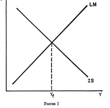
FIGURE I

Figure I shows the familiar IS-LM _{diagram in which the price}

level is assumed constant. The monetary policy problem is viewed as setting the money stock at the level such that the LM function will cut the IS _{function at the full employment level of income, Yf-}

Alternatively, the policy problem could be viewed as in Figure II with the monetary authorities setting the interest rate at r*,' thereby making the LM function horizontal.2 In the deterministic model it obviously makes no difference whatsoever whether the policy pre- scription is in terms of setting the interest rate at r* or in terms of setting the money stock at the level, say M*, that makes the LM function cut the IS function at Yf.

But now consider Figure III, in which the IS function is ran-

1. The interest rate could be set through a bond-pegging program such as practiced by the United States during World War II. Of course, the level of the peg could be altered from time to time.

(6)

LM

I\

Is

Yf Y

FIGURE II

LMl

LM2

ISI

Is

YO Y. Yf Y2 Y3 Y

(7)

domly shocked and may lie anywhere between IS1 and IS2. On the assumption that the money demand function is stable, if the money stock is set at M* the LM function will be LM1 and income may end up anywhere between Y1 and Y2. However, if the interest rate is set at r*, the LM function will be LM2, and income may end up anywhere between Yo and Y3, a much wider range than Yj to Y2. In Figure III it is clear that there is a problem of the proper choice of the instrument, and that the problem should be resolved by setting the money stock at M* while letting the interest rate end up where it will rather than by setting the interest rate at r* and letting the money stock end up at whatever level is necessary to obtain r*.

LM1

LM LM3

Y1 Yf Y2 Y

FIGURE IV

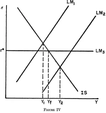
In Figure IV the situation is analyzed in which the IS function is stable but the money demand function is randomly shocked. Set- ting the money stock at M* will lead to an LM function between LM1 and LM2, and income between Y1 and Y2, while setting the interest rate at r* will lead to LM3 and Yf. The interest rate is the proper instrument in this case.

(8)

tions represented by Figures III and IV, it appears that in the gen- eral case the solution of the instrument problem depends on the rela- tive importance of the random disturbances and on the slopes of the IS and LM functions, i.e., on the structural parameters of the system. With these general ideas in mind, it is now possible to proceed to a formal model.

III. A STATIC STOCHASTIC MODEL

Let us begin by presenting a nonstochastic linear version of the Hicksian IS-LM model depicted in Figure I. The model has the two equations

(la) Y=a,+alr, al <0

(lb) M=bo+bY+b2r, b1>O. b2<O

and the variables are all in real terms.3 Equation (la), the IS- function, is obtained by combining linear consumption and invest- ment equations with the equilibrium condition Y=C+1. In equa- tion (ib), the LM-function, the left-hand side is the stock of money and the right-hand side is the demand for money. The parameters are not necessarily constant for all time; they may change as a result of fiscal policy measures and other factors. What is assumed is that the parameters are known period by period.

The model has two equations and three variables, Y, M, and r. Monetary policy selects either M or r as the policy instrument so that there are two endogenous variables and one exogenous variable, the policy instrument. Equations (2) and (3) are the reduced forms for the interest rate and money stock instruments, respectively.

(2a) Y=a,+alr

(2b) M= bo+aobl+ (ajbj+b2) r.

(3a) Y= (ajbj+b2)-1 [aob2+al (M-bo)] (3b) r = (ajbj+b2) -1[M-bo-aob1].

With a desired level of real income of Yf,4 from the reduced

forms for income we obtain the optimal values for the instrument, r* or M*, respectively, as given by equations (4) and (5).

3. It can be assumed either that monetary policy can control the real stock of money, at least in the short run, by altering the nominal stock or that the price level is fixed. Alternatively, it could be assumed that the variables in the model are all money magnitudes; in this case, the desired level of income, Yt, discussed below in real terms, would become instead the desired level of money income such that the economy would be operating at "reasonably" full employ- ment and a "tolerable" rate of price increase. These awkward rationalizations of the economic meaning of the model are, of course, the result of working within a simple model with only the one goal variable, national income.

(9)

(4) r* =a,-(Yf-a,)

(5) M* = a-1 [ Yf (alb +b2) -a0b2+aibj].

It is obvious from (2b) that if r = r*, then M = M* and from (3b) that if M = M*, then r =r*. The policies represented by M = M* and r = r* are equivalent in every way; the choice of a policy instru- ment can be a matter of convenience, preference, or prejudice, but not of substance. In general, the same argument holds for more complicated deterministic models including variables such as free reserves and the level of bank credit.5

Now consider the model obtained by adding stochastic terms to the deterministic model above. The model becomes

(6a) Y=ao+alr+u

(6b) M=bo+bY+b2r+v

whereE[u] = E[v] = 0

E[u2] =-oU2; E[V2] =OV2

E [uv] = o0uv = pu-vouv.

In this model the level of income is a random variable, and in gen- eral its probability distribution will depend on whether the money stock or the interest rate is selected as the policy instrument.

It is natural to argue that the selection of the instrument should depend on which instrument minimizes the expected loss from fail- ure of the level of income to equal the desired level. Let us assume a quadratic loss function 6 SO that the expected loss, L, is given by

(7) L=E[(Y-Yf)2].

It can easily be shown that if the interest rate is the instrument, the minimum expected loss is obtained when r = r* as given by equa- tion (4) ; similarly, if the money stock is the instrument, the optimal money stock is M=M* as given by equation (5) .7 Once the instru- ment has been selected, the model is one of certainty equivalence under the loss function of equation (7), and the optimal policy in the stochastic model is identical to the optimal policy in the determinis- tic model.

However, as can be seen from the reduced forms (8) and (9) for interest rate and money stock policies, respectively, in the stochastic

5. In the model presented there is one goal variable and one instrument to be chosen from two possible instruments. In more complicated models, say where there is a choice of two out of three possible instruments and one goal variable, the optimal policy will lie along a line connecting the two instruments chosen. When a point on this line is selected, the value of the variable rejected as an instrument will be determined by the model.

6. See H. Theil, Optimal Decision Rules for Government and Industry (Amsterdam: North-Holland, 1964), pp. 2-5, for some comments on the reasons for using a quadratic loss function.

(10)

model the two policies are not equivalent as they were in the deter- ministic model since the stochastic terms of the reduced form equa- tions will depend on which instrument is selected.

(8) Y=ao+alr+u

= Yf+u when r=r*

(9) Y= (aibj+b2)-'[aob2+aj (M-bo) +b2u-aiv]

= Yf + (albl+ b2) - (b2u-alv) when M = M*.

By substituting (8) into the loss function (equation (7)), we obtain the minimum expected loss, L, under an interest rate policy, and by substituting (9) into the loss function, we obtain the minimum ex- pected loss, LM, under a money stock policy, as given by equations

(10) and (11). (10) Lr= cru2

(11) LM= (ajbj+b2) -2 (ai2,V2-2puvalb2fUov +b22o,52).

Equation (11) has some interesting implications for the impor- tance of the interest sensitivity of the demand for money.8 From

(11) we find that

(12) aZ)Lm _{=2aj(ajbj+b2)}-3ffaua b2 (biau+PU'v

-a, (+ blpv)

If b12+pUV < 0, thenD L X > when b2 < 0.9

What this means is that the higher is the interest sensitivity of the demand for money (the lower b2 is algebraically), the lower is the minimum expected loss from a money stock policy. The intuitive explanation for this result (which may on first thought seem pecu- liar) is as follows: first, note that this result requires puv <0, which means that there is a tendency for disturbances in the two sectors

8. If the model is log linear, then b, is the interest elasticity of the de- mand for money.

9. This result can be seen as follows. First, note that b1 - + pu < 0 can

Tu ag~~~~T

only occur if pug <0. Multiplying b1- + p"u by - and observing that

0t, pug O'u

b, _{0fv b} c,

<bi pu, since -1 puw<O and bi>0, we find that 0<- + <

pug Gcu Putg au

+ bi pub, Thus, in (12) the term (- + b1 puv) is positive if (b, - + puv) is DLM

(11)

to be simultaneously expansionary or contractionary. Second, note that aV must be relatively large compared to b1jo-,. Under these condi- tions the effect on income of the relatively large disturbances in the monetary sector is smaller, the larger is the interest sensitivity of the demand for money. As will be shown below, in this situation an interest rate policy is superior to a money stock policy.

Another aspect of the interest sensitivity is that in general Lm is at a minimum at a nonzero value of b2 which may be negative, which means that in some cases a small amount of interest sensitivity is better than none. This fact can be seen by setting (12) equal to zero to find the extremum. The second order conditions assure that this extremum is always a minimum. It is then found that for b2<0

at this minimum, it is necessary that puv+ b1?> 0 and bip.V+? > 0.

Uv cu

It can also be shown that at this minimum a money stock policy is superior to an interest rate policy. Since the conditions for a min- imum Lm to occur at b2 <0 are likely to be met in practice, these re- sults suggest that some interest sensitivity may well be better than none. Indeed, as shown in the next section this fact may be exploited by deliberately introducing an interest-sensitive supply of money into the model.

The two policies may now be conveniently compared by con- sidering the ratio of their expected losses.

(13) LM = (ajbj+b2) 2( a,22 2puvajb2UV +b22)

Lr au Tu

It could be argued that much more is known about the monetary sector than about the expenditure sector so that at the current state of economic knowledge UV2 is much smaller than UoU2. As can be

seen from equation (14), if rv/cru is small enough (av/u < b1 is suffi- cient) the ratio Lm/Lr will be less than one so that a money stock policy would be superior to an interest rate policy.

(14) L _{= (abl+b2)(} 2a2 2puvalb2 +b22)

(a~bi~2) 2~ 2 2-

Lr

au4

(u

= _(ajbj+b2) -2 _[(a,-+b2 _)22ajb2? (1+puv)]

< (alb1+b2) 2( alr+b2 2

(12)

which instrument is optimal may vary over time if the structural and stochastic parameters change.

This analysis, based on the size of r may be compared to the Friedman-Meiselman view that monetary policy is superior to fiscal policy because velocity is more stable than the investment multiplier.' In fact, in the model of (6) fiscal policy and an interest rate policy are equivalent in terms of their effects on income since

in (6a) fiscal policy affects the term a, while an interest rate policy

affects the term air. But it is important to note that the condition at,<r, is not alone sufficient to insure the superiority of the money stock policy.

The stochastic model is one of certainty equivalence in the decision sense but not in the utility sense. Whichever instrument is selected, the optimal decision is the same in the stochastic model as in the certainty model. However, the stochastic model is not equiv- alent in the utility sense since the level of disutility is zero in the certainty model but nonzero and dependent on the choice of the policy instrument in the stochastic model.

The stochastic terms in the model may be interpreted as arising from a one-period lag in data availability on the level of income. If income data were available instantaneously, then random dis- turbances would show up immediately in terms of their effects on income, and the policy instrument could be adjusted accordingly, assuming, of course, that policy actions took effect instantaneously. But if information on the goal variable becomes available with a lag, the instantaneous feedback principle is no longer applicable, and it is necessary to think of the goal variable as being a function of the instrument. For monetary policy problems it seems quite reasonable to think of information on money and interest as being continuously available while information on income is available only with a lag.

Thus, the time subscripts on Y, M, and r are all identical in (6a) and (6b), but Yt is not observable until t+1.

Lags in the effects of policy actions may or may not produce a model analytically equivalent to (6a) and (6b); it is necessary to specify the nature of the lags. If production, consumption, and money demand decisions are made one period in advance, the model might be

(13)

Yt+1 = ao+alrt+ut+l

Mt= bo+bYt+i+b2rt+vt+i.

This model is analytically equivalent to (6a) and (6b). The money demand function may appear a bit strange, but it is possible that the amount of money demanded this period is based on production plans made this period which will determine next period's income.

IV. THE COMBINATION POLICY

It will be recalled that under the money stock policy there is an optimal value for b2, the interest sensitivity of the demand for money. Since it would be a most unlikely coincidence for the actual value of b2 to equal the optimal value, it should be possible to obtain the optimal slope to the LM function by making the supply of money interest sensitive. Whether the supply of money should be positively or negatively related to the interest rate will depend on whether the slope of the LM function with a fixed money stock is too high or too low.

Consider the policy defined in terms of setting values for c', and C'2 in a money supply equation2 given by M= c'l + c'2r. How- ever, because the denominators of the optimal c'1 and c'2 vanish for certain parameter values, it is convenient to define the money supply function by equation (15) where co is set equal to the com- mon denominator of the optimal c'1 and c'2.

(15) coM=c1+c2r.

When (15) is added to the model, there are three equations and three unknowns - Y, r, and M - and the expected loss is minimized by setting the partial derivatives of the loss with respect to c1 and c2 equal to zero. The policy instruments may then be said to be the values of c, and c2. We find that the optimal policy is given by

(16) c0M= cl*+c2*r,

where co= bio.2+ a,.

c1* = cO (bo+ biYf) + (Y1-ao) (aV2+ blaru)

C2* = cob2- a1 (ov2+ blorfs).

Under this combination policy the stochastic term in the reduced form equation for income is affected so that the minimum expected loss, L0, is found to be

(17) Lo or+2UV 2lpuv2)

(14)

In equation (16) it can be seen that the combination policy becomes a pure interest rate policy when c,=O, and becomes a pure money stock policy when c2* - 0 3It should be obvious that except in these special cases in which either co or c2 vanish, the combination policy is superior to both of the pure policies.4

The expected losses under the combination policy may be sub- stantially less than the expected losses under either of the pure policies.5 The explicit specification of a combination policy allows the "fence-sitters" in the debate to stay on the fence and to feel superior in doing so. However, the success of the combination policy depends on knowledge of the parameters of the model, and the com- bination policy depends on knowledge of more parameters than does a pure money stock or a pure interest rate policy. Furthermore, it is clear from equation (16) that optimal monetary policy may require the central bank to introduce either a direct or an inverse relationship between M and r since the c, and c2* coefficients may be of either the same or opposite signs. Equation (16) is compli- cated enough that intuition in this matter is to be distrusted; a com- bination policy based on intuition may be worse than either of the pure policies.

V. A DYNAMIC MODEL

The analysis may be extended to more complicated models in which there are lagged responses to the disturbances and policy actions. Considerations involving an investment accelerator or a dependence of consumption on lagged income may produce a model such as

(18a)

Yt=ao+ajrt+Sjyt-1+S2yt-2+Ut

3. When there are no disturbances in the monetary section (oa 2 = au = Q)

the optimal policy is to make the supply function of money the same as the demand function for money at the full employment level of income. At the other extreme, when there are no disturbances in the expenditure sector

(au2 = au-, = 0), the optimal policy is to set the interest rate at the level required for full employment. These results were anticipated by Martin Bailey, National Income and the Price Level (New York: McGraw-Hill, 1962), pp. 154-62. However, in discussing the more general case when disturbances may appear in both sectors, Bailey argues that the source of any particular disturbance, and therefore the proper direction in which to adjust the money stock, may be de- termined by seeing whether income and interest move together or inversely. This policy prescription is not applicable if, as assumed in this paper, income is observed with a lag.

4. A proof is presented in the Appendix.

(15)

(18b) Mt= bo+bYt+b2rt+vt

where E [ut] = E [vt] = 0

E _[utu8,-r2 when t =s, = 0 when t7rs

E [vtv8] =_2 when t= s, = 0 when t:7s

E [utvs] = a when t = = 0 when _t7Ls.

Since lagged responses are picked up by the lagged income terms, it is assumed that the disturbance terms are serially independent.

At time t, assuming that Yt-1 and Yt-2 are known, the model may be considered as identical to the model without lags except that the constant term in the IS equation becomes

aO+SiYti1+S2Yt_2.6

Period by period, then, the optimal level of each of the three policies is given by the same expressions as before except that the constant term ao in these expressions is replaced by ao+S1Yt-1+S2Yt_2. It is easy to see that if any one of the policies is followed period by period the dependence of income on lagged income will be elimi- nated.7

A policy adjusted period by period might be called an "active" policy. Professor Friedman has argued that a successful active policy is impossible given the current state of knowledge, and that we would be better off with a steady rate of growth of money regard- less of current conditions. Such a policy might be called a "passive" policy. The model of this paper involves no economic growth, and so the analog to Friedman's proposal is a money stock fixed per- manently. We may also consider a permanent interest rate policy.8 Friedman's position is based on his contention that the lags in the effects of monetary policy are long and variable, and so it may 6. At this stage of the argument it would be a trivial matter to add lagged income terms to the money demand equation or lagged interest rate terms to either or both equations. These terms could all be incorporated into the con- stant terms. While the later analysis would not be affected in any fundamental way by adding lagged income terms to the money demand equations, the presence of both lagged income and lagged interest terms would make the algebra later on difficult and perhaps impossible.

7. In the combination policy, ct* (though not co and c2*) is itself a random variable depending on Yt-1 and Yt-2, and it is therefore necessary to see whether c1* has a finite mean and variance. If it did not, the policy would presumably not be feasible. However, it is easy to see that cl* does have a finite mean and variance. The mean and variance of cl* depend on the means and variances of Yt-l and Yt_2 which in turn depend on the means and variances of the distur- bances in periods t-1 and t-2, but in no earlier periods since the dependence of Y on lagged Y is eliminated by the optimal combination policy. Therefore, it is clear that the mean and variance of c1* exist, and the same argument applies to the interest rate and money stock policies.

8. A third possibility is a permanent combination policy, but I have not worked out the algebra. However, my conjecture is that co and C2* would have

(16)

well be unfair to analyze the merits of his position within the model given by (18). However, this model does seem to have some rele- vance to the problem. First, note that Friedman's position does not depend per se on existence of lags in the effects of monetary changes, but rather on the inability to predict the level of income at the time when monetary actions take effect regardless of whether or not this effect occurs with a lag. The longer and more variable the lag, of course, the less accurate are income predictions likely to be. The dynamic model of (18) includes both predictable income changes through the influence of the lagged income terms and unpredictable income changes through the influence of the random terms, and so does represent, at least in part, the nature of the problem that led Friedman to his position.

The second aspect of this model to be noted is that the timing relationship between turning points in money and income is variable due to the random terms u and v even though the partial effect of money on income does not have a variable lag. Thus, the model is consistent with Friedman's findings on the variability of the lag between turning points in money and income.9 Friedman's argument for a constant rate of growth in the money stock depends on varia- bility in the partial effects of money on income. In passing, it might be mentioned that the only way to obtain evidence on the variability of the partial effects of money on income would be to show either that in a model of the economy the estimated regression coefficients were statistically significantly different from one period to another, or that the variability in the lag in turning points could not occur in a model with constant partial effects of money on income unless a most improbable probability distribution of the disturbance terms existed.

In analyzing passive policies, consider first the interest rate policy of setting r= r permanently. It is optimal to set the interest rate according to

(19) ro = al-l [Yf (1-Si-S2)-ao],

and, substituting this expression into (18a), we have

Yt-yf=S1(ytl-1yf)+S2(yt-2- Yf) +Utor (20) Zt-S1Zt-1-S2Zt-2=Ut, where Zt= Yt- Yf.

From (20) it can be seen that the level of income follows a second- order Markov process around a base level of Yr.f

9. Milton Friedman and Anna J. Schwartz, "Money and Business Cycles," Review of Economics and Statistics, Vol. 45, no. 1, pt. 2 (Feb. 1963), 32-64.

(17)

To solve (20) we need a particular solution, Zt = _Z't,to (20) and a general solution, Zt = Z't, to its homogenous counterpart

(21) Zt-SlZt-1-S2Zt-2=0, Zt=Zt-Zf1.

A particular solution to (20) may be found by assuming that

(22) Zt= I QkUt-k,

k=o

where the Qk are yet to be determined. Substituting (22) into (20)

we have

t t-1 t-2

QkUt-k-Sl 54 QkUt-l-k-S2 I QkUt-2-k-Ut=Ovor

k=o k=o k=o

(23) (Qo-1 ) ut+ (Q1-SiQo)utI

t

+ I (Qk-SlQk-1-S2Qk-2)Ut-k=0. k=2

For (23) to be satisfied for all possible values of Ut-k, the coefficient

of each Ut-k must be zero. In order to find a general expression for Qk, we must solve the difference equation

(24) Qk-SlQk-1-S2Qk-2=0, k==2,3, ....

Equation (24) has the same form as (21) and so its solution provides both the particular solution and the solution to the homogenous counterpart except that the arbitrary constants differ. The general solution to (20) has the form

Zt = _z'_t+z't

= I QkUt-k+Z~ t

k=o

and involves one of the three cases below. Case 1: S2 > -4S2

Solution: Qk=AXl1k+A2x2k

Zfk=Bllk+B2X2k

where Al = 1/2 (S+?VS12+4S2)

X2=1/2 (S1-JS12?4S2)

Case 2: S12 4S2

Solution: Qk= (Al+kA2) (1/2S1)k Zfk= (Bl+kB2) (1/2S1)k

Case 3: S12 <-4S2 (i.e. S2 < (S 2)

Solution: Qk= (-S2) k2k(Al cos k O+A2 sink 6) Zfk= (-S2) 2k (B1 cos

k

G+B2 sin

k 0)

where tan =-4S2-S12 V

(18)

The constants A1 and A2, which differ from one case to another, are determined by solving the two equations,

Q0-1=0

Q1-S1Q0= 0.

Similarly the constants B1 and B2 are obtained by solving the two equations

Z'o 0= S1Z-+S2Z-2

Zf1 = (S12+S2) Z1?+SlS2Z_2,

where Z-1 and Z-2 are the initial conditions on income.

The stability conditions on the solution are for Case 1 that jSi1 <1-S2, for Case 2 that

IS1!

<1, and for Case 3 that _1S21<1. If the solution is stable the initial income conditions will have a smaller and smaller effect on income as time goes on, and the un- conditional mean and variance of Zt will approach

(25) E[Zw]=E[:$ QkUt-k]=0 k=o

00 00

(26) Var[Z] =E[Z2.] =E[( E QkUtak)2]=u2U Q2k.

k=o k=o

If the stability conditions are not met, the effect of the initial condi- tions on income will not disappear and the unconditional variance will grow without limit. Since Zt = _Yt-_Yf,_{the variance of Zt gives}

the expected loss with the loss function used before. Even if the loss is defined - _{i.e., less than infinity}- under the passive interest rate

policy, the loss will be greater perhaps far greater -than under the optimal active policy.2

Now consider a policy of permanently fixing the money stock at Mt= M0. With the optimal value of M0 we have

(27) Zt=RZt-1+R2Zt-2+wt

where R1=Slb2(ajb1+b2) 1

R2= S2b2(ajbj+b2) '

wt= b2 (aibj+b2) -1(b2ut-ajvt). Let the particular solution be

t

(28) Zt= I PkWt, k=o

where the Pk are determined by the solution of a difference equation analogous to (24). The general solution also has the same form as before and the stability conditions on R1 and R2 are the same as on 2. Under an active interest rate policy the expected loss is 0r2 from (10). But from (23) it is clear that Qo = 1 _sothat the difference of the losses is

00 00

a.U22 I~ QA;oou~ 2_ f2=a2 2 r1u X 1 Qk k > > 0. O

(19)

S, and S2 above. However, since 0 < b2 (ajb+ b2) -1 <1 under

normal assumptions as to the signs of a,, b1, and b2, it is clear that

jR11 < _{IS11 and}jR2J < IS21. This means that although the variance of income might not exist under either policy it is possible that the variance exists when the money stock is set, but not when the interest rate is set. But note that if the variance exists under the interest rate policy, it may be lower than the variance under the money stock policy, since in the latter case we have

00

(29) E [Zoo2] = U,2 X Pk2

k=o

When one compares (26) and (29), it is clear that 4Pk2 is smaller

than lQk2, but Urw,2 may be larger than ,,2.

In comparing the active and passive policies, it is clear that the expected loss under the passive policy is greater than under the active policy. While the optimal active and passive policies were in both cases derived under the assumption of known parameters, even if the parameters are not known exactly the analysis suggests that a nonoptimal active policy may still be superior to an optimal passive policy. With incomplete knowledge, a sensible procedure might be to start from a base policy of a fixed money stock (which is most likely superior to a fixed interest rate), and then to move away from this base somewhat cautiously in implementing an active policy.

VI. CONCLUDING OBSERVATIONS

The choice of instruments problem is clearly a consequence of uncertainty, and analysis of the problem requires a stochastic model. The basic model of this paper is the simplest possible model within which the nature of the problem can be carefully defined and a solution determined. It is obvious that while the model provides some insight into the solution of the problem as faced by practical policy- makers, its main value is in clarifying the nature of the problem and suggesting an approach which might be applied to more complete and realistic models.

(20)

possible to construct a plausible stochastic model in which the property tax stabilized income better than an income tax with the same expected revenue.

Except for a few passing comments no attention has been paid to the very important problem of the effect of uncertainty as to the values of the parameters of the model. In principle what should be done is to treat each parameter as a random variable,3 but in even the simple model of this paper this approach is analytically intract- able due to the large number of variances and co-variances involved, and the existence of products and ratios of random variables in the reduced form equations. A more promising approach might be to employ a sensitivity analysis to see how the results based on known parameters would differ if the parameters differed by plausible amounts from the estimates used in the analysis.

APPENDIX

It is necessary to prove that L0 ? Lr and L,-iLm. Without loss of generality we may assume that au= av since in equation (6a), the IS-function, it is possible to measure Y and u at rates (annual, quar- terly, and so on) selected so that au= o,; such a change in units will also require adjustments in some of the parameters. In the proof, no separate notation will be introduced for the adjusted parameters, it being understood that the appropriate adjustments have been made. Under the assumption that au= ut, it can be seen from (10) and

(17) that

0 Le

(lpuv2) 1 (puV) 2 (

Lr 1+2puvbl+b,2 (l puv2) + (puv+bl)2

?1 for - l'puv<1.

If bi = 1, the denominator in (30) vanishes at puv 1. However, if bi 1 we may write

Le (1 -puv2) (1-puv)

- ~~~= 1for puv=1.

Lr 2(1+puv) 2

Under the assumption that au = av, it can be seen from (11) and (17) that

(31) Le - (alb, + b2)2 (1 -_p2uv)

LM

(a12-2

puv aib2

+

b22) (1 + 2 publ + b2)

(alb, + b2)2 (1 - puV)

(alb, + b2)2 (1 - puv2) + _[(a,- _b1b2)₊_puv_(aibi- _{b2) ]2} c 1 for - 1 ' puv ? 1.

If b1= 1, the denominator in (31) vanishes at puv =-1, and if a, = b2, the denominator vanishes at put = 1.

(21)

If b, 1, we may write

Lc (a + b2) 2 (1 - PUV2)

LM

(al +

b2) 2 (1- puv2) + [(a, - b2) (1 + puv) ]2 (a, + b2)2 (1 - puv)

(al + b2)2 (1 - puV) + (a, - b2)2 (1 + puv) = 1 at puv = - 1.

If a = b2,we may write

Le

a,2 (b1

+

1)2 (1 -PUV2)

Lm a,2 (b1 + 1)2 (1 - Puv2) + [(a, - _{alb1) +puv (alb} - _a,)]2

(b, + 1)2 (1 + puv)

(b, + 1)2 (1 + puv) + (1 - b1)2 (1 - puv) = 1 atpuv = 1.