Exchange Rate
∗
Carlos Eduardo Gonçalves
†
, Bernardo Guimarães
‡
Contents: 1. Introduction; 2. A Simple Model; 3. Estimation; 4. Results; 5. Concluding remark.
Keywords: Exchange Rate, Default, Monetary Policy, Identification through Heteroskedasticity.
JEL Code: F3, E5.
In a country with high probability of default, higher interest ra-tes may render the currencylessattractive if sovereign default is costly. This paper develops that intuition in a simple model and estimates the effect of changes in interest rates on the exchange rate in Brazil using data from the dates surrounding the monetary policy committee mee-tings and the methodology of identification through heteroskedasticity. Indeed, we find that unexpected increases in interest rates tend to lead the Brazilian currency to depreciate.
Em um país onde é alta a probabilidade de calote, aumentos da taxa de juro podem gerar depreciação da moeda local caso o default seja um evento custoso. Esse artigo desenvolve um modelo simples que capta esse efeito e estima o impacto de variações de juros sobre a taxa de câmbio no Brasil usando dados em torno das reuniões do Copom e a metodologia de identifi-cação via heterocedasticidade. Com efeito, nossos resultados sinalizam que, no Brasil, elevações inesperadas dos juros geram em média depreciações da taxa nominal de câmbio.
1. INTRODUCTION
Economists usually take for granted that higher domestic interest rates lead to a currency appreci-ation. This is reflected both in undergraduate Macroeconomics textbooks1and in policy debates.2 This
paper argues that, under certain conditions, higher interest rates may not render the domestic currency
∗We thank Mauro Rodrigues, John Taylor, an anonymous referee, and several seminar participants for helpful comments, Homero
Guizzo and Marcio Pajes for able research assistance.
†Universidade de São Paulo, Department of Economics. E-mail:[email protected] ‡Escola de Economia de São Paulo, FGV. E-mail:[email protected]
1See, for instance, Blanchard (2005, pages 424–5).
2The policy of high interest rates in the US in the early 1980’s are still referred to as the strong Dollar policy. In general, monetary
more attractive. If defaults are costly, the relationship between interest rates and the exchange rate is not monotonic, and depends on the relation between interest rates and default risk. We formalize this argument and present empirical evidence that higher interest rates may indeed turn the domestic currencylessattractive using Brazilian data.
But how can higher interest rates turn the domestic currency less attractive? Higher interest rates are promises to pay more, so how can a promise to pay more reduce theexpectedpayment and, conse-quently, the value of the domestic currency?
The reason is the following: debt default is associated with output losses.3 Those losses reduce
the amount of collectable taxes and hence the resources available for repayment. Higher interest rates imply higher odds of a default. Thus, increasing interest rates has two opposite effects: the first is to increase repayment if debt is honored, and the second is to reduce the expected amount of available resources due to the higher expected costs stemming from a greater probability of default.
One could think that the second effect would never dominate, but it need not be so. If a large chunk of tax revenues has to be spent on some inflexible government expenditures, as is the case in Brazil, small shocks in tax revenues imply large fluctuations of net resources available for repayment.
The second effect may dominate if the odds of default are large. This will be the case when in-terest rates and the level of indebtedness are high enough. We develop this intuition in a simple model in which the association between interest rates and the exchange rate will display a U-shaped form: initially, increasing interest rates strengthens the currency, but after an endogenously determined threshold it leads to a depreciation.
The inverted relationship between interest rates and the exchange rate is not a mere theoretical curiosity. Using Brazilian data from the 2000/2006 period we find that higher than expected interest rates are associated with currency depreciations, which is contrary to conventional wisdom.
Brazil is a clear example of an economy where our theoretical result of an inverted relationship between interest rates and the exchange rate may hold. In the last few years, Brazil has been a world-wide champion of high interest rates, rarely missing first or second place. Since 2003,realinterest rates have been hovering around 10% a year although the Brazilian EMBI risk measure has been on aver-age around 4%. Moreover, the debt to GDP ratio in this period was higher than the averaver-age of other emerging economies (around 50%).
We estimate the effect of interest rates on the exchange rate in Brazil using data from the dates surrounding the monetary policy committee meetings. In tackling the problem empirically, a first con-cern is to avoid the usual endogeneity and reverse causality problems that plague this sort of study. For that, we resort to Rigobon and Sack’s (2004) methodology of identification through heteroskedasticity using data from the days immediately preceding, and immediately following, the monthly meetings of the Monetary Policy Committee (Copom hereafter).
Indeed, we find evidence that upward shocks to the interest rates tend to lead the Brazilian currency todepreciate. An increase of 100 basis points in interest rates leads to an average depreciation between 0 and 2%. During the 2000/2006 period the uncovered interest rate parity (UIP) was upside down in Brazil. This result is consistent with the theoretical prediction of our model if we assume that in the period studied, the Brazilian economy was at the “wrong” side of the U-shaped curve. It would be interesting to estimate the relation between those variables for low debt and low interest rates, but the post-1999 period was marked by high debt and real interest rate levels only. Hence, it is not possible to empirically identify the other side of the U-shaped curve.
The economic literature has already shown that the ability of monetary policy to control inflation may be hindered in some situations. Sargent e Wallace (1981) argue in their seminal article that raising interest rates may lead to increased expected inflation if households anticipate debt will eventually need to be monetized due to a greater interest burden. Drazen e Masson (1994) go further and add signalling
3There is wide agreement in the literature that debt default leads to output losses, even though the literature is less clear on
considerations to this analysis. In their model, tight monetary policy helps signalling toughness, which leads to lower expected inflation. However, by increasing unemployment, tight monetary policy also worsens the trade-off faced by the policy maker in the future as long as unemployment has some per-sistence. This second effect may offset the first and lead to higher expected inflation. Blanchard (2005) recent article suggests the possibility of multiple equilibria in the relation between interest rates and exchange rates. In one equilibrium, the traditional UIP holds and in the other it is upside down. Which equilibria best describes the economy depends on the debt levels and risk premia. He concludes by claiming that high indebtedness may cause the inflation targeting system to work poorly in Brazil. The model in Akemann e Kanczuk (2005) is similar to ours since it endogenizes the link between interest rates and the default risk. There, because of what the authors call “political constraints ” the govern-ment has to fulfill a certain primary surplus, and higher interest rates auggovern-ments the probability of a default. However, differently from all these articles we assume neither an exogenous haircut nor that the central bank rescues the government by printing money.
On the empirical front, estimating the effects of monetary policy on asset prices has been the aim of a branch of the literature beginning with Cook e Hahn (1989). Recently, more attention has been devoted to the issue of identification, and the methodology developed by Rigobon e Sack (2004) that we use here is not the only proposed alternative. Zettelmeyer (2004) regresses changes in exchange rates around meeting dates on the changes in interest rates over the same window using the change in the policy rate as an instrument. However, in the case of Brazil, data on the surprise in the policy rate is not available, and the assumption that the choice of the policy rate is not significantly influenced by economic and political news that do affect asset prices in general may be a bit too strong due to the high frequency and magnitude of shocks that hit the Brazilian economy. We hence opted for the methodology of identification through heteroskedasticity.4
Some papers have aimed at estimating the relationship between exchange rates and monetary pol-icy in emerging countries during times of crisis.5 Our study focuses on a similar question but the data analyzed is not confined to a crisis period. The effects presented here refer to the bulk of the time Brazil has been following an inflation targeting regime.
The rest of the paper is organized as follows: in Section 2 we present a simple model showing that the impact of changes in interest rate on the exchange rate depend on initial indebtedness. In Section 3, we present the econometric methodology and explain its key underlying assumptions, and in Section 4 we present the results. Section 5 concludes.
2. A SIMPLE MODEL
In this section we propose a simple model in which the relationship between interest rates and the exchange rate is not monotonic. Similar to the workings of a traditional Laffer curve, the exchange rate initially appreciates as the interest rate rises but after a threshold it depreciates as the risk of default effect more than offsets the direct effect. The purpose here is not develop a structural model to be estimated later in the empirical part of this work. The idea is simply to ilustrate our point more formally.
Consider a small open economy in which the government – fiscal authority – inherits a certain amount of debt,b. The Central Bank independently decides the level of the interest rate. The domestic bond is subject to a default risk because the government is unable to cut expenditures below a certain
4In any case, regressions using the short term rate as an instrument also yield a negative association between interest rates and
the value of the Brazilian currency.
5In particular, Caporale et alii (2005) estimate the impact of monetary policy on the exchange rate during the Asian crises.
minimum level,gm, and total tax revenues,τ, are unknownex ante(only its distribution,F(τ), the minimum and maximum levels,τmandτM, are known). This uncertainty about government resources stems from the fact that tax revenues depend on the behavior of stochastic variables like the pace of economic activity and relative prices, which are unknown when investment decisions are made.
If total debt service plus minimum expenditures happen to be below tax revenues, that is, ifτ > Rb+gm, the government fully honors its claims. But if they turn out to be greater than total tax revenues, the government partially defaults, allocatingτ−gmto the debt service. If taxes just cover gm, total default ensues.
We assume that before increasing expenditures abovegm, the government prioritizes debt repay-ment, as τ−gmis the maximum the government could possibly allocate to debt service. That as-sumption has no bearing on our qualitative results and quantitatively it reduces the negative impact of higher interest rates on the exchange rate through the risk of default channel – thus it works against the fiscal dominance/Laffer curve effect.
We also assume that there is a floor on government expenditures,gm. There are two ways to justify that assumption. First, and this applies clearly to the Brazilian case, some expenditures may be constitutionally mandatory and hence out of the Executive’s discretionary reach. In Brazil, these expenditures amount to nearly 90% of total revenues. Second, it may be politically inviable to severely cut government outlays beyond a certain level. For instance, the incumbent party may ruin its chances of staying in power after the next election (or face risks of being ousted by social turmoil) if it does not provide a minimum amount of public goods.
Default periods, however, bring costs to the country. Those costs reduce public resources by a factor γ, where 0 < γ < 1, leaving the government with (1−γ)τ in disposable revenues. This is a usual assumption in the literature (since Cohen e Sachs, 1986) and is consistent with the data: countries that default usually experience falls in GDP. One theoretical rationale justifying these costs is that creditors have to sanction defaulting countries if equilibrium debt is to be positive (Bulow e Rogoff, 1989). Another rationale is that the private sector may be less willing to invest if it becomes unsure about government’s commitments to honor contracts. And finally, some amount of revenues may end up being squandered in the form of transaction and negotiation costs.
Investors are risk-neutral and can purchase either domestic bonds with a contractual gross return of Ror international risk-free securities payingR∗. So the following non-arbitrage condition must hold:
eF
eS.R∗= (1−F(Rb+gm))R+
Z Rb+gm
τm
(1
−γ)τ−gm b
f(τ)dτ
whereeF is the future nominal exchange rate,eS is the nominal spot exchange rate. In our model, there is no coordination between monetary and fiscal policy. The monetary authority chooses interest rates with the sole objective of achieving the inflation target, and its decision is not influenced by the fiscal stance. The fiscal authority, in turn, is passive: it simply decides whether or not (and to what extent) to default based on the minimum expenditure constraint,g≥gm.
In the non-arbitrage condition, it is usually assumed thateF is pinned down by long-term funda-mentals and all variations in the right-hand side of (1) are reflected in changes ineS.A milder and more realistic assumption – which we employ here – is thateF is less elastic thaneS to variations on the right-hand side of equation (1).
The crucial question for us is: what happens to the right-hand side of the above equation – and thus toeS – when there are changes inR?
∂rhs
∂R = (1−F(Rb+gm))−Rf(Rb+gm)b+ (Rb(1−γ)−γgm)f(Rb+gm)
∂rhs
∂R = (1−F(Rb+gm))−γ(Rb+gm)f(Rb+gm) (1)
Because the first term is positive and the second is negative, the sign of ∂rhs
∂R – and therefore of ∂eS
∂R – is undetermined.
IfRbis small, the effect of interest rates on the value of the currency is positive. On the other hand, ifRbis high and the probability of default is close to 1, the effect becomes negative and increases in interest rates cause the currency to depreciate.
The relation betweeneS andRdepends on the probability distribution ofτ. SpecializingF(.)as
F = τ−τm
τM −τm
, equation (1) yields:
∂rhs
∂R =
τM−(Rb+gm)
τM −τm −
γ(Rb+gm) τM −τm
= τM −(1 +γ)(Rb+gm) τM−τm
.
It follows that:
∂eS
∂R < 0⇐⇒Rb <
τM
1 +γ−gm= (Rb) thr
and
∂eS
∂R > 0⇐⇒Rb >
τM
1 +γ−gm= (Rb) thr
The relation betweeneSandRis hence U-shaped. Higher interest rates lead the currency to appre-ciate for lower values ofRbbut weaken the currency ifRbis higher than the thresholdRbth.
Higher interest rates are promises of more payment to creditors in the future. If the government is using all available resources to pay debt up toRb, how can a higherR generate lower expected repayment? The reason is that a higherRincreases the probability that the government may be forced to renege on this promise, which is costly. Therefore, a higher Rhas a negative impact on the size of the expected amount available for repayment. This can be seen in equation (1). The first term (1−F(Rb+gm))captures the traditional effect: higher interest rates appreciate the exchange rate by increasing the return to holding domestic bonds. This effect occurs only if there is no default, so it is less important as the probability of default increases. The second term, equal to−γ(Rb+gm)f(Rb+gm), reflects the reduction in the expected amount available for repayment. If the debt issue is unimportant, this is small and so the adverse impact is negligible, but ifRbis high and the probability density of obtaining revenues just enough to coverRb+gmis large, the negative effect of interest rates on the value of the currency may dominate the first effect.
Importantly, the fiscal dominance region may not be negligible. Ifgmaccounts for a large chunk of τM, then the threshold(Rb)thris not very high. The reason is the following: as the default costs reduce the whole tax revenues (τ) and a large part of that has to be used to financegm, the impact of default on the resources available is magnified. The proportional fall on the amount available for repayment,
1−(1−τγ)τ−gm −gm
=γ τ
τ−gm ,
may be substantially bigger thanγbecause the term multiplyingγmay be large. In the case of Brazil, inflexible government expenditures are around 90% of the tax revenues, so τ
τ−gm
than 10.6So even a smallγmay translate into a large reduction in available resources and hence a large
haircut.7
As we mentioned above, the assumption that all the money abovegmwill be used to pay debt is an extreme one – if the government decides to default, it might as well decide to default a bit more, as it will have to pay some fixed default costs anyway – and that would enlarge the fiscal dominance region. We do not pursue this debate further, however, because it is difficult to obtain accurate quantitative implications from this model. Our point is simpler: any kind of default costs may turn the relationship betweenRandeupside down, and the higher the costs (or the higher the expenditure abovegmin case of default) the “earlier” this shift will occur. This relationship depends onRb: higherRand higher bincrease the probability of falling on “wrong side” of the U-shaped curve.8
3. ESTIMATION
The model presented in the last section shows that default costs may in theory turn thee−R relationship upside down ifRbis above a certain threshold (a kind of fiscal dominance result). In this section, we provide some empirical evidence that higher interest rates can indeed lead to a currency depreciation.
An important difficulty in obtaining reliable estimators is that identification problems – reverse causality and omitted variables – seem to be acute in this case. Hence we need a coherent identifi-cation strategy to estimate the relationship between variations in the interest rate and variations in the exchange rate consistently. Using data on these variables around the days the monetary policy committee (Copom) meets, our strategy will be to apply Rigobon and Sack’s (2004) methodology of identification through heteroskedasticity.
3.1. Monetary policy in Brazil
After abandoning a currency peg regime in 1999, the Brazilian Central Bank (BCB hereafter) opted to target inflation and let the exchange rate float. Under the new regime, the BCB has been following with rigor the usual procedures of accountability and communication. These include, among other things, a monthly meeting of its monetary policy committee (Copom, hereafter), almost always on the third Wednesday of the respective month, when a decision on the prime rate is reached by a board of directors.9
The Copom’s monthly decision about the prime rate undoubtedly exerts a strong influence on long term interest rates by suggesting what the BCB plans to do in the future, and it is precisely the greater variability of interest rates on those dates that allows us to isolate causation by instrumenting through heteroskedasticity.
Despite the successful results in terms of price stability, there is a raging debate, both in the media and within academic circles, concerning the desirability of the Brazilian Central Bank’s (BCB’s) policy. Whereas on one side some economists criticize the high interest rate policy based on “fiscal dominance” type of concerns, others say high rates are a consequence of Brazil’s poor track record on price stability
6See Mendes (2008).
7Other effects could top this up. For instance, a higherRmay cause less investment, and hence less output and tax revenues,
regardless of whether there is default or not.
8The model could be re-interpreted in terms of inflation: if debt goes above the level that can be sustained with tax revenues
(τ), the government prints money to repay debt. But inflation has costs, as the economy gets less productive, people shift from producing to minimizing cash in hand. In this monetization version these costs are captured by the parameterγand an inverted relationship between the spot exchange rate and the interest rate would come through the effect of higher inflation on the future exchange rate.
and argue that “excessive toughness” may be needed to signal serious inflation aversion.10 It is
under-standable that Brazilian bonds have yields far above the proverbial risk-free US Treasury notes. What is puzzling, however, is that Brazilian interest rates have been substantially and consistently higher than the US Treasury billsplusBrazil’s own EMBI risk measure. Is the BCB simply getting it wrong?
A related debate concerns the causes behind the appreciation of the Brazilian currency in recent years: many pundits claim the appreciation was a by-product of a tough monetary policy implemented to anchor inflation. But are these claims supported by the data? The answer to this question has serious policy implications for Brazil’s policy makers since one of the channels linking monetary policy to inflation is through its effects on the exchange rate. If the answer is negative, then the case for high interest rates is weakened.
3.2. Data and identification
Our data set goes from January/2000 to December/2006. Because the Copom meetings take place on Wednesdays, our variables are constructed as follows: ∆e = log(ethursday)−log(etuesday)and ∆i = log(1 +ithursday)−log(1 +ituesday).11 The sample, consisting of values of∆eand∆i, is
divided in two subsamples: the subsampleCcorresponds to the dates when the Copom meets, and the subsampleN corresponds to dates (same week days) with no meeting. The number of observations in each of the two sets is denoted byTCandTN, respectively.
In order to identify the effect of interest rates on the exchange rate, it is not enough to evaluate their correlation (or run an OLS regression) because of endogeneity problems (the interest rate and the exchange rate are influenced by each other) and the presence of omitted variables in the regression (the interest rate and the exchange rate are influenced by other common variables). The following system of equations captures these features.
∆et = α∆it+zt+ηt (2)
∆it = β∆et+γzt+εt (3)
where∆itis the change in the 1-year interest rate,∆etis the change in the spot exchange rate,ztis an omitted variable,εtis a monetary policy shock andηtis a shock to the exchange rate.
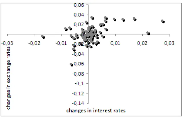
Figure 1 shows a positive correlation between the change in the exchange rate (∆e) and the vari-ation of the interest rate (∆i) around Copom meetings. A simple OLS regression yields apositiveand significant coefficient, which suggests UIP may be upside down.
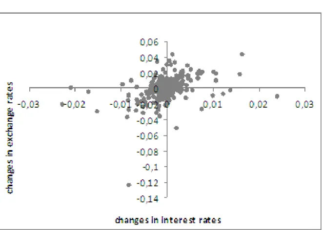
However, this correlation reflects not only the impact of interest rates on exchange rates, but pos-sibly also the effect of exchange rates on the interest rate. Figure 2 shows a similar pattern for the Non-Copom dates data.
The key question is whether the positive correlation in Figure 1 is driven solely by the factors that also lead to a positive relationship between∆eand∆iin Figure 2 or not. The methodology of identifi-cation through heteroskedasticity allows us to disentangle those effects, making use of the fact that on Copom dates there is an extra shock to interest rates (the decision of the Central Bank) which is absent in non-Copom dates.
3.3. Methodology
In order to circumvent the endogeneity and omitted-variables problems, we use the methodology of identification through heteroskedasticity proposed by Rigobon e Sack (2004). The key assumption is
Figure 1:∆e×∆i, Copom dates
that the variance of the shock to the interest rate (εt) in the dates belonging to setCis higher than the variance of the shock to the interest rate in the dates belonging to setN, while the variances ofηtand ztare equal:
σC
ε > σNε σηC = σNη
σzC = σNz
We also assume thatzt,εtandηthave no serial correlation and are uncorrelated with each other. As shown in Rigobon e Sack (2004), the assumptions on the behavior of the variability of shocks in the two subsamples allow us to identifyα. The intuition is the following: in dates where Copom meets, there is a shock to equation 3,σεincreases, but there are no shocks to other variables. So, the overall relation between∆eand∆ishould be different between the two subsamples,CandN.
Solving for the reduced form of equations 2 and 3, we reach:
∆it = 1
1−αβ[(β+γ)zt+βηt+εt] (4)
∆et = 1
1−αβ[(1 +αγ)zt+ηt+αεt] (5)
Figure 2:∆s×∆i, Non-Copom dates
∆Ω = σ C ε −σεN (1−αβ)2
"
1 α
α α2
#
In words, becauseσC
ε 6=σεN, the covariance matrix of∆eand∆iis not the same in subsetsCand N and therefore it is possible to identifyαby looking at the difference in the covariance matrix in the two different subsamples.12
Now, consider the following variables:13
12See also Rigobon (2003).
13The results in the appendix of Rigobon e Sack (2004) consider the caseT
C =TN. It is trivial to extend them to the more
∆I ≡
∆i′ C
√
TC , ∆i
′ N √ TN ′ (6)
∆E ≡
∆e′ C
√
TC , ∆e
′ N √ TN ′ (7)
wi ≡
∆i′ C
√
TC ,−∆i
′ N √ TN ′ (8)
ws ≡
∆e′ C
√
TC
, −√∆e′N TN
′
(9)
A major result in Rigobon e Sack (2004) is thatαcan be consistently estimated by a standard instru-mental variables approach with the novel instruments,wiandws. Why arewiandwsvalid instru-ments for∆Iat equation 2? Intuitively, vectorwi is correlated with∆Ibecause the bigger variance in the Copom dates implies that the positive correlation between ∆i′
C/
√
TC
and ∆i′ C/
√
TC
more than outweighs the negative one between ∆i′
N/
√
TNand −∆i′N/
√
TN. Formally:
plim1
Tw
′ i∆I =
1 TC
∆i′
C.∆iC− 1 TN
∆i′ N.∆iN
= (β+γ)
2
(1−αβ)2σ C
ε −
(β+γ)2 (1−αβ)2σ
N ε >0
On the other hand,wiis not correlated with eitherzorηbecause the positive and negative corre-lation of each part of the vector exactly cancel each other out:
plim1
Tw
′ iz =
1 TC
∆i′ C.zC−
1 TN
∆i′ N.zN
= β+γ
1−αβσ C
z −
β+γ
1−αβσ N z = 0
plim1
Tw
′
iη =
1 TC
∆i′ C.ηC−
1 TN
∆i′ N.ηN
= β
1−αβσ C
η −
β 1−αβσ
N η = 0
Analogous results are obtained for the instrumentws.
We consider the one-year interest rate as the most appropriate one to the purposes of identifying impacts of monetary policy on the exchange rate. That is because we want a measure that fully captures the information released by the Copom decision without much noise. The one-month interest rate is highly influenced by Copom decisions, but is less informative than the one-year rate. The reason is the following: suppose agents expect the central bank will put an end to a loosening cycle either this month or the next. If it decides to implement the cut this month, the upward surprise in the 1-month rate will be non-negligible, but the surprise in the one-year rate will be fairly small. On the other hand, the same surprise in the one-month rate may be associated with a large impact in the one-year rate if that is due to the central bank signalling a different trend regarding interest rates in the next months. What about longer rates? The two-year or five-year interest rates add little information about monetary policy on the top of the one-year rate and are influenced by many other factors (thus they are noisier).14
14Liquidity is also an important consideration here, as less liquid instruments are noisier, and that would actually rule out
The traditional way of analyzing the impact of “exogenous” monetary policy decisions (the so-called event study approach) is to consider that unexpected changes in the policy rate are exogenous and use those to estimate equation 2. Rigobon e Sack (2004) show that such strong assumptions are unnecessary: with the assumptions on heteroskedasticity, one can consistently estimateα. Here, we argue that the methodology of identification through heteroskedasticity allows us to go one step further by permitting the use of the one-year rate as the regressor. As discussed above, the one-year rate is a better measure of monetary policy surprises, but the problem is that it is clearly endogenous. Using the method of identification through heteroskedasticity, however, we do not need to assume exogeneity. All we need is to assume that the one-year interest rate is directly affected by the Copom decisions but the exchange rate is only affected through the influence of the changes in the interest rate.
3.4. Test of the identifying assumption
Here we show that the variances ofεtand ηt in both subsamples corroborate our assumptions: there is no evidence that channels linking the Copom meetings and shocks toηtare important.
Equations 4 and 5 and the assumptions about variances in the two subsamples lead to:
V ar(∆iC)−V ar(∆iN) = σC
ε −σεN
(1−αβ)2 >0 (10)
V ar(∆eC)−V ar(∆eN) = α2 σC
ε −σεN
(1−αβ)2 >0 (11)
Equations 10 and 11 show that the variances of∆iand∆emust increase in Copom dates but since the variance of∆eis substantially larger than the variance of ∆i, the proportional increase in the variance of∆emust be smaller.
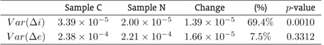
Table 1: Variances of∆iand∆e
Sample C Sample N Change (%) p-value V ar(∆i) 3.39×10⁻⁵ 2.00
×10−5 1.39
×10−5 69.4% 0.0010
V ar(∆e) 2.38×10⁻⁴ 2.21×10⁻⁴ 1.66×10⁻⁵ 7.5% 0.3312
Table 1 shows the variances of∆iand∆ein the two subsamples. Thep-values reported in Table 1 refer to theF-test of equality of variances in both subsamples. We can reject at 1% thatV ar(∆i) does not increase in subsample C. Using the above equations, the estimated change inV ar(∆e) corresponds to a value ofα= 1.1(which coincides with our estimatedα). The main concern regarding our estimation strategy is whether the variance ofηtincreases in Copom dates. This would lead to large increases inV ar(∆e). Fortunately, we cannot reject thatV ar(∆e)is the same in both subsamples, which allows us to proceed with the identification through heteroskedasticity methodology.
4. RESULTS
an unexpected increase of 100 basis point in the interest rates leads to an increase in∆e(that is, a
depreciationof the exchange rate) between 0 and 2% (approximately).
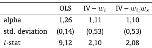
Table 2: IV estimate
OLS IV –wi IV –wi;ws
alpha 1,26 1,11 1,10
std. deviation (0,14) (0,53) (0,53) t-stat 9,12 2,10 2,08
The IV estimation is not highly accurate because the change in the variance of∆iin Copom dates does not increase so much, so the instrumentwiis not very strongly correlated with∆i. Also, as the proportional change in the variance of∆eis small,wsis only weakly correlated with∆i, and including it as an instrument in the regressions does not produce any meaningful change.
The OLS estimation yields a higher coefficient and a smaller standard error. Given the problems of endogeneity and omitted variables discussed above, that is what we should expect because the OLS estimator would be upward biased. Nevertheless, the precision of the estimation does not allow us to assert that the results obtained by the IV and OLS methods are significantly different, so we cannot conclude that the OLS estimator is biased. That is not relevant for the purpose of this paper, though. What is important is that αis positive and significant even when we employ the methodology of identification through heteroskedasticity, which means that the positive coefficient found is not driven by the well known endogeneity biases relating variations in interest rates and variations in exchange rates.
These results are consistent with the predictions of our simple model. Upward surprises in the one-year interest rate generated by the Copom meetings are rendering the Brazilian currencyless at-tractive to investors. Importantly, this finding is not the outcome of any major crisis since during our seven-years sample period the Brazilian economy ran primary fiscal surpluses, implemented inflation targeting and let the exchange rate float freely.
Theoretically, such effect should not be found in countries with lower real interest rates and less debt problems. In Chile, for example, debt is only around 12% of GDP and real interest rates have been around to 2% per year (averages for 2000/2006). Chile also has an inflation targeting regime with periodic meetings of the monetary policy committee to decide the basic interest rate. Unfortunately, the most liquid market rate is the five-year inflation-indexed bond. For our purposes, the data is therefore noisy, because five-year real rates are not strongly influenced by monetary policy decisions. Moreover, the data series is relatively short. Nevertheless, the correlation between changes in real interest rates and changes in the exchange rate is negative in Chile (interest rate increases correspond to currency appreciations), even if it is not statistically significant.15
5. CONCLUDING REMARK
In this paper we showed that if debt and interest rates are both high, unexpected monetary tighten-ings may cause the currency to depreciate, dampening the total effect of monetary policy on agreggate demand and generating an negative externality that is passed to the fiscal authority. This suggests that more monetary and fiscal policy cooperation could enhance total welfare.
BIBLIOGRAPHY
Akemann, M. & Kanczuk, F. (2005). Sovereign default and the sustainability interest rate risk effect.
Journal of Development Economics, 76:53–69.
Blanchard, O. (2005). Fiscal dominance and inflation targeting: Lessons from Brazil. In Giavazzi, F., Goldfajn, I., & Herrera, S., editors,Inflation Targeting, Debt and the Brazilian Experience. MIT Press.
Bogdanski, J., Tombini, A., & Werlang, S. (2000). Implementing inflation targeting in Brazil. BCB Working Papers.
Bulow, J. & Rogoff, K. (1989). A constant recontracting model of sovereign debt. Journal of Political Economy, 97:155–178.
Caporale, G., Cipollini, A., & Demetriades, P. (2005). Monetary policy and the exchange rate during the Asian crisis: Identification through heteroskedasticity. Journal of International Money and Finance, 24:39–53.
Cho, D. & West, K. (2003). Interest rates and exchange rates in the Korean, Philippine and Thai ex-change rate crises. In Dooley, M. & Frankel, J., editors,Managing Currency Crises in Emerging Markets. University of Chicago Press.
Cohen, D. & Sachs, J. (1986). Growth and external debt under risk of debt repudiation.European Economic Review, 30:529–560.
Cook, T. & Hahn, T. (1989). The effect of changes in the federal funds target on market interest rates in the 1970s.Journal of Monetary Economics, 24:331–351.
Drazen, A. & Masson, P. (1994). Credibility of policies versus credibility of policymakers.Quarterly Journal of Economics, 109:735–754.
Favero, C. & Giavazzi, F. (2005). Inflation targeting and debt: Lessons from Brazil. In Giavazzi, F., Goldfajn, I., & Herrera, S., editors,Inflation Targeting, Debt and the Brazilian Experience, 1999 to 2003. MIT Press.
Kraay, A. (2002). Do high interest rates defend currencies during speculative attacks? Journal of Interna-tional Economics, 59:297–321.
Mendes, M. J. (2008). Sistema orçamentário brasileiro: Planejamento, equilíbrio fiscal e qualidade do gasto público. Texto para Discussão 38,Consultoria Legislativa do Senado Federal.
Rigobon, R. (2003). Identification through heteroskedasticity.Review of Economics and Statistics, 85:777– 792.
Rigobon, R. & Sack, B. (2004). The impact of monetary policy on asset prices. Journal of Monetary Economics, 51:1553–1575.
Sargent, T. & Wallace, N. (1981). Some unpleasant monetarist arithmetic. Federal Reserve Bank of Min-neapolis Review, Fall:1–19.
Sturzenegger, F. & Zettelmeyer, J. (2006). Debt Defaults and Lessons from a Decade of Crises. MIT Press.