Analysis stage 3: Finding patterns of interaction

(1)

Paper 049-31

AMMI Macros for Multiplicative Interaction Models

Eun-Joo Lee, Advanced Micro Devices Inc., Sunnyvale, CA

Dallas E. Johnson, Kansas State University, Manhattan, KS

ABSTRACT

When you are faced with analyzing two-way cross-classified experiments, you are almost always interested in whether the two factors interact or not, and if they do interact, combinations of the two factors are responsible for the interaction in the data. When there are no independent replications, there are no traditional tests for interaction. SAS® macros have been developed to provide user-friendly statistical software for the analysis and interpretation of interaction in two-way experiments. These newly developed macros are called the AMMI (Additive Main-effects and Multiplicative Interaction) macros. The AMMI models allow one to analyze two-way data with interaction even if there are no independent replications. In addition to fitting AMMI models and models such as Tukey’s single degree of freedom for nonadditivity Model, and Mandel’s bundle-of-straight-lines model, the macros provide many useful graphical displays including displays that help you determine the pattern of interaction when a pattern exists and that help you decide how many multiplicative interaction terms to include in the model. This paper describes how the AMMI macros can be installed, how they can be used, and the kinds of output they produce.

INTRODUCTION

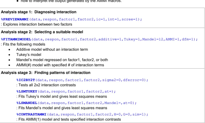
A set of SAS macros called the AMMI macros has been developed to analyze two-way cross-classified experiments without independent replications under the SAS® software release 8.2 (TS2MO) in a windows environment. The AMMI macros consist of six independently executable main macros and 22 sub-macros that are called by the six main macros. The main AMMI macros are given in Figure 1. For information about the models that are fit: See Lee (2004) and/or Milliken and Johnson (1989). This paper shows:

● how to compile and store the AMMI macros on your SAS;

● how to prepare input data prior to calling a macro;

● how to assign parameter values in each macro;

● what may be expected as output from each macro;

● how to interpret the output generated by the AMMI macros.

Analysis stage 1: Diagnosing interaction

%PREVIEWAMMI(data,respon,factor1,factor2,ic=1,int=1,scree=1); : Explores interaction between two factors

Analysis stage 2: Selecting a suitable model

%FITAMMIMODEL_{(data,respon,factor1,factor2,additive=1,Tukey=1,Mandel=12,AMMI=1,dfm=1);} : Fits the following models

• Additive model without an interaction term • Tukey’s model

• Mandel’s model regressed on factor1, factor2, or both • AMMI(#) model with specified # of interaction terms

Analysis stage 3: Finding patterns of interaction

%IC2BY2T_{(data,respon,factor1,factor2,sigma2=0,dferror=0);} : Tests all 2x2 interaction contrasts

%LSMTUKEY(data,respon,factor1,factor2,at=); : Fits Tukey’s model and gives least ssquares means

%LSMANDEL(data,respon,factor1,factor2,Mandel=,at=0); : Fits Mandel’s model and gives least squares means

%CONTRASTAMMI(data,respon,factor1,factor2,H=0,G=0,sim=1); : Fits AMMI(1) model and tests specified interaction contrasts

(2)

COMPILING AND STORING MACRO DEFINITIONS

The AMMI macros are provided as a source file, 'AMMImacros.sas', that can be used in any operating environment. However, some features of the macros may not work properly if you use a prior release of the SAS software rather than the system environment used for developing the macros, which is release 8.2 (TS2MO). Supplying the macros in a text file makes them available for use in other system environments having SAS software release 8.2 such at OS/2, Mainframe, VMS, or Unix.

The provided source file, AMMImacros.sas, consists of 28 macro definitions and a data step to generate the SAS data set named AMMI.EX_L. The data set, AMMI.EX_L, is a table of simulated degrees of freedom associated with multiplicative interaction terms in the AMMI model and it will be referenced, updated, and extended by users when they fit an AMMI model and/or run a new simulation to get a new set of degrees of freedom that depend on the number of rows and columns in the two-way data set.

First, one needs to assign a library named 'AMMI' where the compiled macros will be stored along with the data set AMMI.EX_L. Then, submit the whole program file, AMMImacros.sas, for execution. This compiles and saves the compiled macros in the catalog, AMMI.SASMACR. This compilation occurs only once. One may need to recompile these macros when using them in a different release of the SAS software or in another operating system. Some of the AMMI macros also use macros in the autocall library supplied by SAS Institute. Using the compiled macros in a specific library allows one to distinguish them from any other user-defined macros. Also, it allows one to use the macros currently assigned to the autocall library in a single working session. The library AMMI must be assigned each time you use the AMMI macros along with setting two system options, MSTORED and SASMSTORE=AMMI. The MSTORED system option enables the stored compiled macro facility and the SASMSTORE=AMMI option specifies the SAS data library that contains the catalog of compiled AMMI macros. The following two SAS statements need to be submitted before calling AMMI macros.

LIBNAME AMMI 'SAS-data-library';

OPTIONS sasmstore=AMMI mstored;

SAS-data-library must be a valid physical name for the SAS data library on the host system. The physical name of the SAS data library is the name that is recognized by the operating environment. The physical name must be enclosed in single or double quotation marks: See the LIBNAME statement in SAS® Language Reference: Dictionary for more information. Once the required system options have been set, one can call the AMMI macros.

The file 'AMMImacros.sas' begins with the above two statements and should be placed in the program editor window or the enhanced editor window. Then, submit for execution after replacing 'SAS-data-library' with the user's choice of folder in which to store the compiled macros. The compilation of the AMMI macros must be done prior to trying to execute an AMMI macro. To execute an AMMI macro, one must precede the first macro call by these same two statements.

PREPARING INPUT DATA

The AMMI macros are designed for analyzing two-way cross-classified experiments when there are no independent replications. Identifying the pattern of interaction is also one of the objectives when analyzing two-way experiments using AMMI models. Therefore, the input data must be balanced without any missing treatment combinations. For example, if one has five possibilities for factor 1 and four possibilities for factor 2, then the number of observations in the input data set must be 5×4=20. Otherwise, the program will give an error message and stop running.

Each individual macro in the set of AMMI macros requires three columns of input data: A response variable and two classification variables indicating values for factor 1 and factor 2. One may have more than three columns in the original input data set. The AMMI macros use only three columns specified among them.

Each classification variable can have either a numeric or a character value. The ideal length of character values for labeling purposes in the output is $6 or smaller. One may have values longer than $6 for classification variables, but they will be truncated in some of the output.

RUNNING THE MACROS

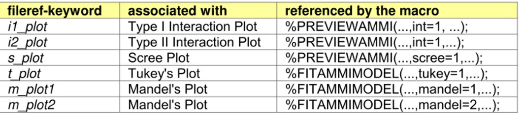
All plots produced by the AMMI macros are generated in an Adobe Portable Document Format (PDF) file before they are shown in the SAS Graph window. If one wants to save the graphic output in a PDF file, FILENAME statements must be assigned before calling the macro that produces the desired graphic output. The file reference keywords that are used within FILENAME statement must be identical to those referenced by the AMMI macros. These are i1_plot for Type I interaction plots, i2_plot for Type II interaction plots, and s_plot for a scree plot. These are all referenced by the macro %PREVIEWAMMI. Others are t_plot for Tukey's plot, m_plot1 for Mandel's plot regressed on factor 1, and m_plot2 for Mandel's plot regressed on factor 2. These are all referenced by the macro %FITAMMIMODEL. The user may select the filenames under which each plot is saved. For example, the statements

FILENAME i1_plot "C:\PDFplots\Type1iPlots.pdf";

FILENAME i2_plot "C:\PDFplots\Type2iPlots.pdf";

(3)

preceding the %PREVIEWAMMI macro will place two Type I interaction plots into the PDF file,

C:\PDFplots\Type1iPlots.pdf, two Type II interaction plots into the PDF file, C:\PDFplots\Type2iPlots.pdf, and the scree plot into the PDF file, C:\PDFplots\ScreePlot.pdf. For another example, the statements

FILENAME t_plot _{"C:\PDFplots\TukeyPlots.pdf";}

FILENAME m_plot1 "C:\PDFplots\Mandel1Plots.pdf";

FILENAME m_plot2 "C:\PDFplots\Mandel2Plots.pdf";

preceding the %FITAMMIMODEL macro will place Tukey's plot into the PDF file, C:\PDFplots\TukeyPlots.pdf, Mandel's bundle-of-straight-lines plot into the PDF file, C:\PDFplots\Mandel1Plots.pdf, when you choose to fit Mandel's model regressed on factor1, and C:\PDFplots\Mandel2Plots.pdf, when you choose to fit Mandel's model regressed on factor2. Each of the filenames in the above examples that are placed in quotes can be changed. The names used in the examples assume you have the folder named ‘PDFplots’ on your C drive. Table 1 shows the list of file reference keywords to be assigned within the FILENAME statements.

Table 1. List of file reference keywords for FILENAME statements

fileref-keyword associated with referenced by the macro i1_plot Type I Interaction Plot %PREVIEWAMMI(...,int=1, ...); i2_plot Type II Interaction Plot %PREVIEWAMMI(...,int=1,...); s_plot Scree Plot %PREVIEWAMMI(...,scree=1,...); t_plot Tukey's Plot %FITAMMIMODEL(...,tukey=1,...); m_plot1 Mandel's Plot %FITAMMIMODEL(...,mandel=1,...); m_plot2 Mandel's Plot %FITAMMIMODEL(...,mandel=2,...);

Each plot takes a whole page in a PDF file with its size proportional to the standard letter sheet, 11" for height and 8.5" for width. Each page of a PDF file may be exported to another type of image file using Adobe Acrobat and if this proportion is used to reduce the size of plots, one can keep the shape of original plots. Exporting graphic output as image files with Adobe Acrobat gives high quality graphs often needed for publication purposes. Most of the SAS graphic output loses its original quality when exported to other types of image files, such as BMP (BitMaP), EMF (Extended Meta File), WMF (Window Meta File), JPEG file interchange format, GIF (Graphics Interchange Format)), TIF (Tag Image File format), PNG (Portable Network Graphics), and etc. The PDF graphic output has the unique property that one gets the same quality of graphics as seen in the SAS Graph window. The following sections show how to assign parameter values to each macro and what may be expected as output from each macro.

THE MACRO %PREVIEWAMMI

The macro %PREVIEWAMMI is designed to explore and diagnose interactions between two factors. It produces a table of all 2×2 interaction contrasts calculated from all possible pairwise row and pairwise column contrasts, Type I interaction plots and Type II interaction plots for a set of two-way cell responses as described in Section 1.7.1 of Milliken and Johnson (1989), and a scree plot plotting the non-zero characteristic roots of the matrix Z’Z or ZZ’, where Z is the residual matrix obtained after fitting an additive model to the two-way data. All output is generated as default output unless suppressed.

%PREVIEWAMMI(data,respon,factor1,factor2,ic=,int=,scree=);

data name of input dataset

respon name of response variable

factor1 name of the first classification variable

factor2 name of the second classification variable

ic= 1: produces a table of all 2*2 interaction contrasts (default)

0: suppresses this output

int= 1: produces Type I and Type II interaction plots (default)

scree= 1: produces a scree plot (default)

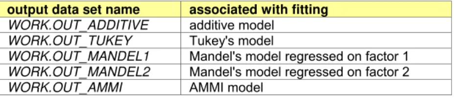
THE MACRO %FITAMMIMODEL

(4)

Table 2. List of output dataset names after fitting models

output data set name associated with fitting WORK.OUT_ADDITIVE additive model

WORK.OUT_TUKEY Tukey's model

WORK.OUT_MANDEL1 Mandel's model regressed on factor 1 WORK.OUT_MANDEL2 Mandel's model regressed on factor 2 WORK.OUT_AMMI AMMI model

%FITAMMIMODEL(data,respon,factor1,factor2,additive=,Tukey=,Mandel=,AMMI=,dfm=);

data name of input dataset respon name of response variable

factor1 name of the first classification variable factor2 name of the second classification variable

additive= 1: fits an additive model (default)

Tukey= 1: fits Tukey's model (default)

Mandel= fits Mandel's bundle-of-straight-lines model

12: regressed on factor1 and factor2, respectively (default)

1: regressed on factor1

2: regressed on factor2

AMMI= #: fits an AMMI model with # of multiplicative interaction terms; must be an integer

1: # of MI terms in AMMI model = 1 (default) 2: # of MI terms in AMMI model = 2 ... if # exceeds the maximum possible, then # = MIN(#(factor1),#(factor2)) - 1

dfm= assigns a method to get degrees of freedom for each of the MI

terms in the AMMI model

1: looks up the table, AMMI.EX_L (default); if searching values

are not in AMMI.EX_L, then dfm=2 is assigned to the macro

2: runs a simulation without storing results

3: runs a simulation and stores results into AMMI.EX_L 4: Gollob's method, (b+t-1-2m) for the m-th MI term

THE MACRO %IC2BY2T

The macro %IC2BY2T is designed to test all 2 by 2 interaction contrasts calculated from all possible pairwise row and pairwise column responses based on a given error variance and its degrees of freedom.

%IC2BY2T(data,respon,factor1,factor2,sigma2=,dferror=);

sigma2= estimate of error variance for testing interaction contrasts dferror= degrees of freedom associated with estimated error variance

THE MACRO %LSMTUKEY

The macro %LSMTUKEY is designed to calculate least squares means for Tukey's model at a specified location along the factor 1 axis in a Type II interaction plot.

%LSMTUKEY(data,respon,factor1,factor2,at=);

factor1 name of the first classification variable factor2 name of the second classification variable

at= location on the factor 1 axis in a Type II interaction plot

(5)

THE MACRO %LSMANDEL

The macro %LSMANDEL is designed to calculate and compare least squares means for Mandel's bundle-of-straight-lines model at a specified location along the factor 1 (factor 2) axis in a Type II interaction plot.

%LSMANDEL(data,respon,factor1,factor2,Mandel=,at=);

factor1 name of the first classification variable factor2 name of the second classification variable Mandel= fits Mandel's bundle-of-straight-lines model

1: regressed on factor1 (default) 2: regressed on factor2

at= location on the factor 1 (factor 2) axis in a Type II interaction

plot where least square means are to be calculated

THE MACRO %CONTRASTAMMI

The macro %CONTRASTAMMI is designed to test user specified interaction contrasts in the AMMI model with only one interaction term. It conducts a likelihood ratio test based on a simulated p-value and simulated critical points after fitting the AMMI(1) model.

%CONTRASTAMMI(data,respon,factor1,factor2,H=,G=,sim=);

H= contrast matrix associated with alpha1 in AMMI(1) model; must be

assigned using braces ({ }) to enclose the values and commas to

separate the rows in parentheses otherwise H=0 is assigned to the

macro

Ex. H=({1 -1 0 0, 1 0 -1 0}) when possibilities for factor1=4

G= contrast matrix associated with gamma1 in AMMI(1) model; must be

assigned using braces ({ }) to enclose the values and commas to

separate the rows in parentheses otherwise G=0 is assigned to the

macro

Ex. G=({1 -1 0 0 0, 1 0 -1 0 0}) when possibilities for factor2=5

sim= 1: runs a simulation to get a p-value and 90% & 95% critical

points for the assigned LR test (default)

0: suppresses simulation

AN EXAMPLE AND SAMPLE OUTPUT

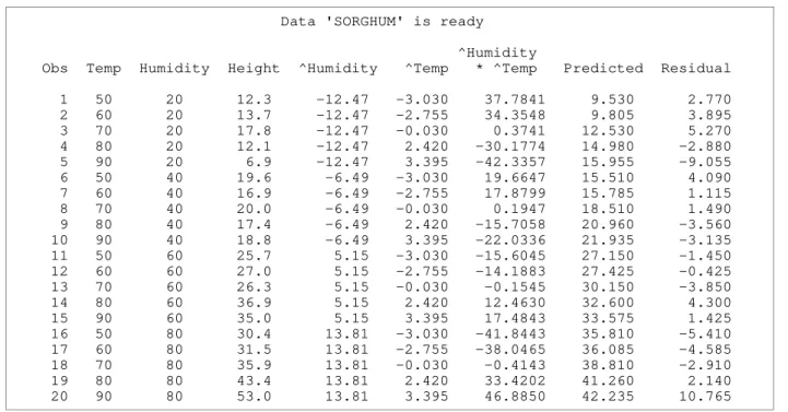
To illustrate results from the AMMI macros, the growth rate of sorghum plants data is used: See Section 1.2 of Milliken and Johnson (1989). The experimenter has 20 growth chambers and conducts an experiment to study the effects of five temperature levels combined with each of four humidity levels on the growth rate of sorghum plants. Most output of the AMMI macros is self-explainable. This section shows some sample output from AMMI macros analyzing the sorghum data.

Either of following macro statements produces the same output.

%PREVIEWAMMI(SORGHUM,Height,Humidity,Temp); or

%PREVIEWAMMI(SORGHUM,Height,Humidity,Temp,ic=1,int=1,scree=1);

Table 3 shows the ready dataset for analyses and this shape of dataset will be produced by every main macro previously shown in Figure 1. The macro calculates an additional five columns based on information in the first three columns provided in the input data which is referenced for subsequent analyses. The column labeled '^Humidity' contains the differences between humidity main effect means and overall mean. The column labeled '^Temp' contains the differences between temperature main effect means and overall mean. The column labeled '^Humidity * ^Temp' is the product of ^Humidity and ^Temp. The column labeled 'Predicted' and 'Residual' are predictions and residuals from an additive two-way model, respectively.

(6)

Table 3. Ready dataset for analyses

Data 'SORGHUM' is ready

^Humidity

Obs Temp Humidity Height ^Humidity ^Temp * ^Temp Predicted Residual

1 50 20 12.3 -12.47 -3.030 37.7841 9.530 2.770 2 60 20 13.7 -12.47 -2.755 34.3548 9.805 3.895 3 70 20 17.8 -12.47 -0.030 0.3741 12.530 5.270 4 80 20 12.1 -12.47 2.420 -30.1774 14.980 -2.880 5 90 20 6.9 -12.47 3.395 -42.3357 15.955 -9.055 6 50 40 19.6 -6.49 -3.030 19.6647 15.510 4.090 7 60 40 16.9 -6.49 -2.755 17.8799 15.785 1.115 8 70 40 20.0 -6.49 -0.030 0.1947 18.510 1.490 9 80 40 17.4 -6.49 2.420 -15.7058 20.960 -3.560 10 90 40 18.8 -6.49 3.395 -22.0336 21.935 -3.135 11 50 60 25.7 5.15 -3.030 -15.6045 27.150 -1.450 12 60 60 27.0 5.15 -2.755 -14.1883 27.425 -0.425 13 70 60 26.3 5.15 -0.030 -0.1545 30.150 -3.850 14 80 60 36.9 5.15 2.420 12.4630 32.600 4.300 15 90 60 35.0 5.15 3.395 17.4843 33.575 1.425 16 50 80 30.4 13.81 -3.030 -41.8443 35.810 -5.410 17 60 80 31.5 13.81 -2.755 -38.0465 36.085 -4.585 18 70 80 35.9 13.81 -0.030 -0.4143 38.810 -2.910 19 80 80 43.4 13.81 2.420 33.4202 41.260 2.140 20 90 80 53.0 13.81 3.395 46.8850 42.235 10.765

Table 4. Table of all 2×2 interaction contrasts

2 by 2 Interaction Contrasts: Y(i1,j1)-Y(i1,j2)-Y(i2,j1)+Y(i2,j2)

Factor Levels Level #: Values

Humidity 4 1: 20 2: 40 3: 60 4: 80

Temp 5 1: 50 2: 60 3: 70 4: 80 5: 90

Humidity (j1,j2)

Temp

(i1,i2) 1,2 1,3 1,4 2,3 2,4 3,4

1,2 1,3

1,4 -2.0 11.4 13.2 13.4 15.2 1.8 1,5 4.6 14.7 28.0 10.1 23.4 13.3 2,3

2,4 2.1 11.5 13.5 9.4 11.4 2.0 2,5 8.7 14.8 28.3 6.1 19.6 13.5 3,4 3.1 16.3 13.2 13.2 10.1 -3.1 3,5 9.7 19.6 28.0 9.9 18.3 8.4 4,5 6.6 3.3 14.8 -3.3 8.2 11.5

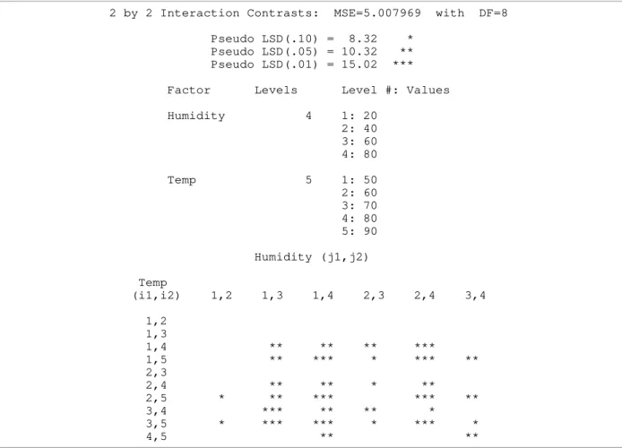
The following macro statement produces the Table 5, which gives a significance test for each 2×2 interaction contrast given in Table 4 using the estimate of the error variance from Mandel's model along with its degrees of freedom.

%IC2BY2T(SORGHUM,Height,Humidity,Temp,sigma2=5.007969,dferror=8);

(7)

significance at the 1% level as test results. An examination of Table 5 indicates that there is no interaction between temperature levels 50, 60, and 70 and humidity as suggested by the examination of Table 4.

Table 5. Results from testing all 2×2 interaction contrasts

2 by 2 Interaction Contrasts: MSE=5.007969 with DF=8

Pseudo LSD(.10) = 8.32 * Pseudo LSD(.05) = 10.32 ** Pseudo LSD(.01) = 15.02 ***

Factor Levels Level #: Values

Humidity 4 1: 20 2: 40 3: 60 4: 80

Temp 5 1: 50 2: 60 3: 70 4: 80 5: 90

Humidity (j1,j2)

Temp

(i1,i2) 1,2 1,3 1,4 2,3 2,4 3,4

1,2 1,3

1,4 ** ** ** *** 1,5 ** *** * *** ** 2,3

2,4 ** ** * ** 2,5 * ** *** *** ** 3,4 *** ** ** * 3,5 * *** *** * *** * 4,5 ** **

Either of following macro statements produces the same output.

%FITAMMIMODEL(SORGHUM,Height,Humidity,Temp,Mandel=1); or

%FITAMMIMODEL(SORGHUM,Height,Humidity,Temp,additive=1,Tukey=1,Mandel=1,AMMI=1,dfm=1) ;

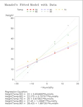
Table 6 shows two ANOVA tables produced after fitting Mandel's bundle-of-straight-lines model. The first ANOVA table partitions the interaction sums of squares from Mandel's model into a portion corresponding to Tukey's model and the remainder labeled "Test for Concurrency". The test for concurrency is a test as to whether the lines fitted by Mandel's model intersect in a single point. Here the F-test for concurrency is F=4.77 (p=0.0343) indicating that Mandel's model is a better fit to the data than Tukey's model. The second ANOVA table gives Mandel's test for interaction as F=17.99 (p=0.0005) which indicates there is significant interaction in these data. Figure 2 gives a Type II interaction plot along with lines predicted by Mandel's model and also shows the equations of the fitted lines from Mandel's model for each temperature.

Table 6. Results from fitting Mandel's bundle-of-straight-lines model

Test for Concurrency of Mandel's Model - line for each Temp Height = Mu + Humidity + Temp + Lambda*^Humidity*^Temp + Temp*^Humidity

Dependent Variable: Height

Sum of

Source DF Squares Mean Square F Value Pr > F

(8)

Error 8 40.063751 5.007969 Corrected Total 19 2611.362000

R-Square Coeff Var Root MSE Height Mean 0.984658 8.940668 2.237849 25.03000

Sum of

Humidity 3 2074.298000 691.432667 138.07 <.0001 Temp 4 136.617000 34.154250 6.82 0.0108 Tukey's Interaction Term 1 288.652009 288.652009 57.64 <.0001 Test for Concurrency 3 71.731240 23.910413 4.77 0.0343

The MANDEL'S Model: Height = Mu + Humidity + Temp + Temp*^Humidity Interaction Term Regressed on Humidity Effect

Sum of

Model 11 2571.298249 233.754386 46.68 <.0001 Error 8 40.063751 5.007969

Corrected Total 19 2611.362000

Sum of

Humidity 3 2074.298000 691.432667 138.07 <.0001 Temp 4 136.617000 34.154250 6.82 0.0108 Mandel's Test for Interaction 4 360.383249 90.095812 17.99 0.0005

Least Squares Means at hat_Humidity=0

Height Standard LSMEAN Temp LSMEAN Error Pr > |t| Number

50 22.0000000 1.1189246 <.0001 1

60 22.2750000 1.1189246 <.0001 2

70 25.0000000 1.1189246 <.0001 3

80 27.4500000 1.1189246 <.0001 4

90 28.4250000 1.1189246 <.0001 5

Least Squares Means for Effect Temp t for H0: LSMean(i)=LSMean(j) / Pr > |t| Dependent Variable: Height i/j 1 2 3 4 5

1 -0.17379 -1.89586 -3.44414 -4.06029 0.8664 0.0946 0.0088 0.0036 2 0.173787 -1.72207 -3.27035 -3.88651 0.8664 0.1234 0.0114 0.0046 3 1.895856 1.72207 -1.54828 -2.16444 0.0946 0.1234 0.1601 0.0624 4 3.444139 3.270352 1.548283 -0.61615 0.0088 0.0114 0.1601 0.5549 5 4.060292 3.886506 2.164436 0.616153

(9)

Figure 2. Type II interaction plot and lines predicted by Mandel’s bundle-of-straight-lines model

Table 7 shows an ANOVA table after fitting an AMMI model with one interaction term. The row labeled 'MI1' gives the interaction sum of squares as 360.8099 with degrees of freedom, 8.2938, which is simulated by the macro. An approximate F-test for interaction is F=4.07 (p=0.1058). Test for interaction in the AMMI model is not significant whereas interaction test given by Mandel's model is highly significant. This is likely due to the fact that Mandel's model provides a much better fit to these data than the AMMI model. The estimates of the parameters in this model are given at the bottom of Table 7.

Table 7. Results from fitting an AMMI model with one interaction term

The AMMI(1) Model: Height = Mu + Humidity + Temp + MI1*Alpha1*Gamma1 DF read from the table AMMI.EX_L

Sum of Pseudo

Source DF Squares Mean Square F Value Pr > F*

Model 15.294 2571.724876 168.154734 15.72 0.0109 Error 3.7062 39.637124 10.694815

Corrected Total 19 2611.362000

Sum of Pseudo

Source DF Squares Mean Square F Value Pr > F*

Humidity 3 2074.298000 691.432667 64.65 0.0011 Temp 4 136.617000 34.154250 3.19 0.1534 MI1 8.2938 360.809876 43.503566 4.07 0.1058

Parameter Estimate

MI1 18.995

Alpha1 -0.616 -0.302 0.225 0.692 (Humidity 4) (20) (40) (60) (80)

(10)

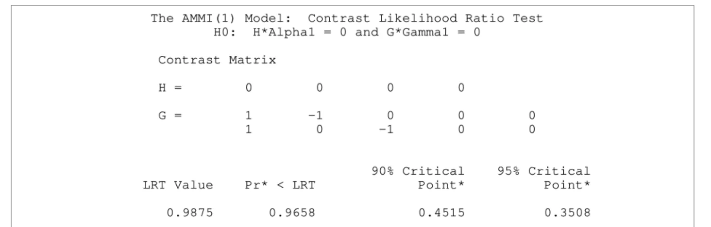
The following macro statement produces the output shown in Table 8 along with the ANOVA table comes from fitting an AMMI model with one interaction term as shown in Table 7.

%CONTRASTAMMI(SORGHUM,Height,Humidity,Temp,H=0,G=({1 -1 0 0 0, 1 0 -1 0 0}));

This statement test whether temperatures 50, 60, and 70 interact with humidity.

Table 8. Results from testing interaction contrasts in an AMMI model

The AMMI(1) Model: Contrast Likelihood Ratio Test H0: H*Alpha1 = 0 and G*Gamma1 = 0

Contrast Matrix

H = 0 0 0 0

G = 1 -1 0 0 0 1 0 -1 0 0

90% Critical 95% Critical LRT Value Pr* < LRT Point* Point*

0.9875 0.9658 0.4515 0.3508

NOTE: 90% and 95% simulated critical points depend on the ranks of H and G as well as the number of levels of each factor. One rejects if the LRT value is smaller than the critical point.

CONCLUSION

The AMMI macros provide three stages of analytic tools; pre-analysis for diagnosing interaction, model fitting for selecting a suitable model, and testing interaction contrasts for finding patterns of interaction in the data. Identifying the pattern of interaction is also one of the objectives when analyzing two-way experiments using AMMI models. Therefore, the input data must be balanced without any missing treatment combinations of two factors.

Software for analyzing interaction in two-way experiments is not currently available for wide-spread use. It is hoped that the developed SAS macros will provide a data analysis tool to researchers needing to analyze two-way nonreplicated experiments. This application will allow many researchers to use multiplicative interaction models to describe real-life phenomena and might accelerate development of new methods related to this area of research. The AMMI macros are available at http://www.k-state.edu/stats/facultypages/ammi_macros.htm along with a user's manual.

REFERENCES

Lee, Eun-Joo (2004). Statistical Analysis Software for Multiplicative Interaction Models. Unpublished doctoral dissertation, Kansas State University, Kansas.

Milliken, G. A., & Johnson, D. E. (1989). Analysis of Messy Data, Volume 2: Nonreplicated Experiments (2nd ed.). New York: Chapman & Hall.

CONTACT INFORMATION

Your comments and questions are valued and encouraged. Contact the authors at: Eun-Joo Lee Dallas E. Johnson Advanced Micro Devices Inc. Kansas State University One AMD Place, MS 79 Department of Statistics Sunnyvale, CA 94088-3453 Manhattan, KS 66506 Work Phone: 408-749-2411 785-532-0510 Fax: 408-774-7499 785-532-7736 E-mail: eunjoo.lee@amd.com dejohnsn@ksu.edu

SAS and all other SAS Institute Inc. product or service names are registered trademarks or trademarks of SAS Institute Inc. in the USA and other countries. ® indicates USA registration.