Electricity price forecasting utilizing machine learning in MIBEL

(1)

Departamento de Ciências e Tecnologias da Informação

Electricity price forecasting utilizing machine learning in MIBEL

João Filipe Ferreira Januário

Orientador:

Professor Doutor Luís Miguel Martins Nunes ISCTE-IUL

Co-orientador: Doutor Nuno Pinho da Silva,

R&D NESTER

(2)

I

Abstract

Short term electricity price forecasts have become increasingly important in the last few decades due to the rise of more competitive electricity markets throughout the globe. Accurate forecasts are now essential for market players to maximize their profits and hedge against risk, hence various forecasting methodologies have been applied to electricity price forecasting in the last few decades. This dissertation explores the main methodologies and how accurately can three popular machine learning models, SVR LSTM and XGBoost, predict prices in the Iberian market of electricity. Additionally, a study on input variables and their relationship with the final price is made.

Keywords

(3)

II

List of Figures

- CRISP-DM Framework ... 5

- Example of spot market clearing price ... 8

- Average price of electricity for a day during cold and warm months in MIBEL ... 12

- Example of an SLP ... 20

- Activation Functions ... 21

- Example of an MLP ... 21

- Example of a Recurrent Neural Network ... 22

- Example of an LSTM unit ... 23

- Example of an SVM classifier ... 25

- Schematic of a one-dimension SVR model ... 26

- Simple decision tree example ... 27

- Average Price of each hour in 2015,2016 and 2017 ... 31

- Boxplot of Electricity Prices from Monday to Sunday and Holidays ... 32

- Price distribution during cold months (October to March) ... 33

- Price distribution during hot months (April to September) ... 33

- Monthly distribution of Electricity Price during 2015 ... 34

- Average Consumption of each Hour ... 37

- Correlation between Consumption and Electricity prices ... 38

- Distribution of Hourly Consumption levels ... 38

-Distribution of Consumption from Monday to Sunday ... 39

- Daily Average Consumption during hot and cold months ... 40

- Average energy generated from hydropower sources on each hour ... 40

- Correlation between Energy generated by hydropower and electricity price ... 41

- Average energy used for pumping water on each hour ... 41

- Correlation between Water Pumping and Electricity Price ... 42

- Average Energy Generated from Wind on each hour ... 43

- Distribution of hourly Wind energy generation during Hot months ... 44

- Distribution of hourly Wind energy generation during cold months ... 44

(6)

V

- Average energy generated from Biomass on each hour ... 46

- Correlation between Biomass Energy Generation and Electricity Price ... 47

- Average energy generated from Solar Panels on each hour in 2015,2016 and 2017... 48

- Distribution of hourly Solar energy generation during Hot months ... 49

- Distribution of hourly Solar energy generation during Cold months ... 49

- Correlation between Solar energy generation and electricity price ... 50

- Correlation between Electricity Price and Renewable energy generation ... 51

- Average energy generated by Coal on each Hour during 2015, 2016 and 2017 ... 52

-Correlation between energy generated by Coal and electricity price ... 53

- Average energy generated by natural gas on each hour ... 54

- Correlation between energy generated by natural gas and electricity price ... 54

- Correlation between Electricity Price and Non-Renewable Energy generation ... 55

- Correlation between Wind energy generation and wind speed ... 57

- Correlation between Wind energy generation and gust speed ... 57

- Hourly distribution of wind speed ... 59

- Hourly distribution of Gust Speed ... 59

- Distribution of Hourly gust speed during cold months ... 60

- Distribution of Hourly gust speed during hot months ... 60

- Correlation between Electricity price and Temperature ... 61

- Correlation between Electricity price and Humidity ... 62

- Correlation between Hydraulic Generation and Humidity ... 63

- Correlation between Hydropower Energy Generation and Precipitation ... 64

- Correlation between Electricity price and Precipitation ... 64

- Correlation between Electricity price and Precipitation above 0.1mm ... 65

- Autocorrelation of electricity price with the next hour price ... 68

- Autocorrelation of electricity price after 36 hours ... 68

- Example of data used to predict the last hour of the day-ahead ... 72

- Wind speed cut in and cut out speeds ... 80

– Best input RMSE values for day-ahead LSTM, XGBoost and SVR ... 82

(7)

VI

List of Tables

- Examples of Machine Learning Models Applied to EPF ... 16

- Mean, Standard Deviation, Minimum, and Maximum of hotter months ... 36

- Mean, Standard Deviation, Minimum, and Maximum of colder months ... 36

- AR(1) Results ... 69

- ARIMA results ... 71

-Input Variables ... 73

- Results for day-ahead predictions with LSTM ... 74

- Results for week-ahead predictions with LSTM ... 74

- Results for day-ahead predictions with XGBoost ... 75

- Results for week-ahead predictions with XGBoost ... 75

- Results for day-ahead prediction with SVR ... 76

- Results for week-ahead prediction with SVR ... 76

- Parameters tested for SVR model ... 86

- Scoring for each SVR model tested ... 87

- Parameters tested for LSTM model ... 87

- Scoring for each LSTM Model ... 88

(8)

VII

Abbreviations

AvE – Average error

AvPE – Average Percentage Error

ANN – Artifical Neural Network

AR – AutoRegressive

ARIMA – AutoRegressive Integrated Moving Average

ARMA - Autoregressive moving average

BP – Backpropagation

CRISP-DM - Cross-Industry Standard Process for Data Mining

EPF – Electricity Price Forecasting

ERBFN – Enhanced Radial Basis Function Network

FWV - Fourier Wave Filtering

GARCH - Generalized autoregressive conditional heteroskedastic

LM – Levenberg Marquardt Algorithm

LSTM – Long Short-Term Memory

LS-SVM – Least-Squared Support Vector Machines

LTPF – Long Term Price Forecasting

MAPE – Mean Absolute Percentage Error

MIBEL – Iberian Electricity Market

MLP- Multi-Layer perceptron

MTPF – Medium Term Price Forecasting

OMIE – Iberian Electricity Market Operator

RBF – Radial Basis Function Network

RES – Renewable Energy Sources

RNN – Recurrent Neural Network

SLP – Single-Layer Perceptron

SOM – Self Organizing Map

SR – Scaling Range

STPF – Short Term Price Forecasting

SVM – Support Vector Machine

(9)

VIII TF – Transfer Function

WMAPE – Weekly Mean Absolute Percentage Error

(10)

1

1- Introduction

Forecasting is a term used to define the ability to predict a future event or variable based on the past study of variables that affect the objective of the forecast. In a competitive liberalized power market, it’s vital for all participants to be able to forecast the electricity price with high accuracy to formulate strategies that allow them to bid and sell energy with the lowest risk possible.

Since the early 1990s, various countries began a process of liberalization of energy trade leading to more competitive energy markets, one example being the Iberian market of electricity (MIBEL). Formed in 2007 as a collaboration between the governments of Portugal and Spain, this is an interconnected market with the goal of distributing electricity in the two countries while benefitting the final consumer by promoting a competitive and free market.

The MIBEL includes three levels of trading one of them being long term and the remaining two being short term, the long term option is in the form of bilateral contracts and can span from a few months to a few years, while day-ahead electricity market and intraday electricity market sessions, also known as spot trading, are short term (Pastor, Pinho, & Esteves, 2018) (Szkuta, Sanabria, & Dillon, 1999).

The short-term options consist of a market where participants bid in a shared pool and a market operator clears the price, this makes the price volatile, but it gives all consumers and providers an equal opportunity to maximize the value of their actions in MIBEL. The long-term option is used when companies prefer to avoid the volatility of daily market prices and want to hedge against the risk of participating in the short-term market. The main objective of the electricity market is to decrease the cost of electricity by promoting competition and transparency.

As the market is interconnected energy prices are usually the same in both Portugal and Spain but there might be occasions where they differ due to the physical capability of the network (Pastor et al., 2018).

Short-term trading options are highly dependent on the demand and available offers of energy which in turn makes the short-term electricity market extremely volatile. This

(11)

2 causes the ability to predict prices before-hand to be very valuable in order to maximize the value that the market participants get from the day-ahead electricity market. Providers want to maximize their profit and consumers want to get the highest amount of energy possible at the cheapest price.

Day-ahead trading is especially important due to storing energy for later use not being a trivial matter, as the manufacturing of large-scale batteries is generally considered not economically viable. At the moment the most frequent way of storing energy in MIBEL is through water reservoirs by utilizing excess energy to pump water that is then stored to generate electric power at a later time.

Long term predictions are also valuable, but they are mostly used for strategic decisions such as: 1-) modifying the amount of energy that is traded between regions. 2-) expanding energy generation. 3-) re-planning the distribution network (Szkuta et al., 1999).

The electricity market has been studied extensively over the years, and certain aspects such as load forecasting have had great breakthroughs (Abdel-Aal, 2006) (Dang-Ha, Bianchi, & Olsson, 2017). Electricity price forecasting presents some characteristics that create difficulty when building prediction models, namely: 1-) it is highly affected by the calendar, especially by weekends and holidays where the prices vary when compared to normal weekdays, creating outliers throughout the year. 2-) It is highly affected by the sources of energy in the network. 3-) It affected by seasons because in drier seasons like the summer there is less hydropower energy being generated as opposed to the more humid seasons. 4-) The pricing can vary a lot in the same day, as early morning hours usually present much cheaper prices than afternoon hours. 5-) It is affected by the player’s bidding strategies that, naturally, are not known ahead by the market.

This dissertation will be focused on predicting short term electricity prices in the MIBEL market, using machine learning algorithms which have been demonstrated to have good results when utilized to predict time-series problems (Aggarwal, Saini, & Kumar, 2009) (Jones et al., 1989) (Ruta & Gabrys, 2007) (Ahmed, Atiya, El Gayar, & El-Shishiny, 2010).

Machine learning has been applied to time-series prediction since the ’80s (Jones et al., 1989), and since then these methods have increasingly grown in popularity. Being applied not only to electricity price forecasting but various different real-world scenarios,

(12)

3 including but not limited to financial market predictions, environmental state predictions and reliability forecasting (Sankar & Sapankevych, 2009).

In the latest decades machine learning has proven to have equal or better results than classical statistical models in several different problems due to: 1-) The increase in theoretical understanding of the models. 2-) The number of varied models that have been developed. 3-) The increasingly ease of access to computing power and open-source machine learning libraries (Ahmed et al., 2010).

Several machine learning models have been applied to predict electricity clearing prices in other markets (Weron, 2014), however to the best of our knowledge it is not an extensively explored methodology in MIBEL.

Algorithms that have shown promising results in previous works, namely SVR, LSTM, and XGBoost, were selected in order to compare how each one performs in the MIBEL. Additionally, a baseline was established utilizing AR (1) and ARIMA. Before starting to describe the practical work, an analysis is made to understand which approaches have been proven useful when predicting time series, and more specifically, electricity price time series.

Objectives

This dissertation will be aimed at studying to what extent is it possible to forecast short term electricity prices utilizing machine learning models. The maximum time frame considered will be up to one week and as a comparative baseline other models that have shown good results will be used. It will also be interesting to compare the difference in the quality of the results in the various models as the time horizon is extended, for example, to compare the day-ahead forecast to the 1-week ahead forecast.

The price of electricity is affected by several variables and the importance of each one to the final price is not yet fully understood, variables like the season, the time of the day, power generation, and others are suspected to be highly important to the final price. As such a study will be made as to how the variables identified as potentially important affect the final market price. For this dissertation, the Iberian electricity market will be studied

(13)

4 exclusively and all historical data is aggregated by technology and provided by R&D

Nester.

In short. the following questions can be identified to be resolved in this work: • What are the most important variables that affect electricity pricing?

• Is it possible to forecast short term electricity prices in the MIBEL with “good” results using artificial intelligence models?

• How do the results compare to other types of models? • How does the time horizon affect the forecast quality?

Document Structure

Chapter 2 starts as by describing the methodology utilized in this work followed by giving a brief introduction to the MIBEL market. The remainder of the chapter presents the related work done in electricity price forecasting with a special focus on machine learning.

The theoretical background can be found in Chapter 3 where the main concepts behind the models relevant to the literature and to this dissertation are explained.

Chapter 4 consists mainly of an extensive statistical analysis of all the relevant data to be used in the models.

In Chapter 5 all the experiment definition and results can be found.

In chapter 6 the conclusions can be found as well as a suggestion for further work. An appendix can be found after chapter 6 that contains all the relevant information about the training of each model.

(14)

5

2- Literature review and business

understanding

Development Methodology

In this dissertation, the Cross-Industry Standard Process for Data Mining ( CRISP-DM) (Wirth, 2000) will be used as a development methodology. This framework splits the development process into six separate phases, Business Understanding, Data

Understanding, Data Preparation, Modeling Evaluation, and Deployment.

This is a flexible framework in which the developer can go back and forth between phases as needed to better adjust the final model.

Figure 1 - CRISP-DM Framework (Sharma & Bradford, 2017)

The outer circle shown in Figure 1 represents the idea that data mining can always be bettered, even after deployment the model can always be adjusted with new data to further improve its forecasting ability. Inside the circle, the different phases are represented, each phase can be defined as such:

(15)

6 Business Understanding: Initial phase of the project where the developer needs to

understand the context of the problem that needs to be solved in order to identify potential issues.

Data Understanding: Data exploration phase, in this phase the training data needs to be

studied, in order to identify potential issues (null values, outliers), and to identify subsets that might have unexpected patterns of relationship between each other.

Data Preparation: Treating the data by solving the problems identified in the previous

phase. In addition to this, some data treatment techniques may be experimented in this phase, like normalizing the data or removing certain variables.

Modeling: In this phase, the model is created or adjusted, the model parameters are

calibrated in order to achieve the best results.

Evaluation: After the model from the previous phase is finished training and predicting

a data set, the results need to be carefully analyzed, if the results aren’t good enough then one of the previous phases needs to be adjusted, otherwise the developer moves on to the deployment phase.

Deployment: The deployment phase presents the finished product, usually in the form of

a report.

The business understanding phase can be mostly seen in chapters 1, 2 and 3, where the motivation, objective, context, and scope of the problem are described, along with a description of how the MIBEL works as well as the theoretical background of the machine learning algorithms that will be applied.

The data understanding phase relates to chapter 4, where the statistical analysis of every relevant variable found in the business understanding phase can be seen.

The following phases mostly relate to the practical work presented in chapter 5, where information about the data preparation, model parameters, and result evaluation is found.

(16)

7 The day-ahead market in MIBEL follows a marginal price model. This model aims to keep electricity price as low as possible while completely satisfying the daily market demand.

The agents bid supply and demand offers for the 24 hours of the next day. The selling offers are sorted in ascended order while the buying offers are sorted in descending order. Sessions are closed at 11:00 (GMT +0) in the previous day (D-1). The MIBEL spot market operator OMIE announces the clearing prices for each hour of the next day, taking into account the curve intersection between the supply curve (generated from aggregated supply bids) and the demand curve (generated from aggregated demand bids). Additionally, some adjustments might be needed to make sure the physical network is able to handle the load without fail (Pastor et al., 2018).

Non-renewable energy providers need to pay coal or gas in order to generate electricity. Renewable energy providers on the other hand, generate electricity from sources in nature like the wind or the sun and as a result they do not have to pay for their primary energy sources. This results in renewable energy providers being able to provide cheaper offers than non-renewable providers.

As the market follows a marginal price model this means that the last bid to match the demand will define the final price for each hour. That price is then the price that all transactions occur independently of the initial bidding price. This means that all providers will satisfy demand at the exact same price as long as their offer is lower or equal to the intersection between the supply and demand curves. As renewable energy providers sell at cheaper prices than non-renewable energy providers, they enter the market first and can sometimes completely fulfill the market demand.

(17)

8

Figure 2 - Example of spot market clearing price ( neighbourpower.com/blog/solar-deregulated-power-market/)

As can be seen in Figure 2 non-dispatchable load generation such as wind and solar have the lowest supplier prices and critical appliances such as light, heating or telecommunication have the highest demand prices. The intersection between the two curves is where the marginal price for each hour is defined. This process occurs for every hour.

Literature Review

The purpose of an organized electricity market is to match the supply and demand of electricity to determine the market-clearing price (Weron, 2014). In the MIBEL participants can conduct their business in the day-ahead electricity market or in the form of bilateral contracts between companies.

In the day-ahead electricity market, the participants bid supply and demand for the 24 hours of the next day to a common pool, the sessions for the day-ahead market are always closed in the previous day at 11:00 (GMT +0). The spot market operator OMIE announces

(18)

9 the clearing price for each hour of the next day with the selling offers being sorted in ascending order while the buying offer being sorted in descending order.

In addition to the day-ahead electricity market, bilateral contracts are utilized by companies to hedge against the day-ahead electricity market risk and to make sure they are able to satisfy their needs in the long term, in bilateral contracts the buyer and the seller negotiate directly and agree on the distribution of a fixed amount of energy at a fixed price during a certain amount of time.

Publications on electricity price forecasting started roughly around the year 2000, prior to this date there is almost no literature on this topic, steadily increasing for the next few years and having doubled in 2005 and then tripled in 2006 when comparing to 2002 numbers. For the next few years there was a steady increase in publications about this topic, with a slight drop-off in numbers in 2010, and then a huge increase in 2012 and the following years (Weron, 2014).

Articles utilizing machine learning techniques for electricity price forecasting have increased tremendously in the past decade, when compared to the prior decade where most articles focused on developing statistical models. This is due to the increasing ease of access to computing power and open software machine learning libraries, which has caused the research community to have a renewed interest in this topic as it is yet an unsolved problem that can potentially be solved or at least vastly more understood utilizing machine learning algorithms.

It is not obvious that machine learning algorithms are able to outperform other methods of prediction, mainly due to each study utilizing different datasets, different software implementations and different evaluation models (Weron, 2014), as such this section will include studies on other methodologies besides machine learning.

Electricity price forecasting

Accurate forecasts don’t guarantee profits and there is always risk in trading in the MIBEL market due to the high volatility of prices (Aggarwal et al., 2009). Since the price is directly related to the amount of energy in the network traded between suppliers and

(19)

10 consumers there is also an interest in the prediction from a viewpoint of the network managers in order to better plan how the network will operate.

Electricity price is a time-series, which means that the series is defined as a consistent sequence of electricity prices over a period of time. Electricity price forecasting is the capability to predict the price of energy at one or more points in time. This prediction is complex seeing as there are multiple variables that affect the final price, and some of them like load forecasting are also complex to predict.

Predictions can be classified into short-term price forecasting (STPF), medium-term price forecasting (MTPF) or long-term price forecasting (LTPF) (Singh, Husain, & Mohanty, 2016). Short-term predictions allow companies to formulate strategies to optimize their participation in the spot market, while medium-term and long-term strategies allow companies to adjust their overall strategy. This may include the overall level of production in the case of suppliers, bilateral contracts with other companies, planning investments, among others (Aggarwal et al., 2009).

The horizon of STPF is between an hour to a week, while MTPF and LTPF range from a few weeks to a few months and a few months to several years respectfully. The purpose of each horizon will be detailed further in the next subsections.

Short-term price forecasting

Short-term forecasts are essential for the players that participate in the spot market. Producers need to forecast energy prices in order to formulate their strategy for participation in the market but also to better optimize the scheduling of their electrical resources to maximize profits.

Investment decisions in renewable generation in the current European regulatory framework with reduced subsidies may leverage short-term price forecasting to simulate markets and compute realistic cash flows in market simulations. For example, short-term price simulation can be used as input in the R&D Nester’s renewable portfolio simulator (Pastor et al., 2018).

(20)

11 Due to energy generally not being a storable resource, consumers need to be able to take advantage of the cheapest moments to get the maximum amount of usable energy. This means that consumers need to have an active participation on the market to satisfy their daily needs while wanting to minimize their risk as much as possible (Catalão, Mariano, Mendes, & Ferreira, 2007).

Medium-term and Long-term price forecasting

Medium-term and long-term price forecasting are very important to the overall electricity market. Most notably, these help strategize when to form bilateral contracts with other companies in order to maximize their profits while satisfying their needs. MTPF and LTPF are also important for other activities such as, generation expansion planning, maintenance scheduling and overall investing (Torbaghan, Motamedi, Zareipour, & Tuan, 2012). For network managers, these predictions help them to better plan how the network will need to change over time and to monitor distribution safety.

Doing medium and long-term predictions is an incredibly complex task, seeing as short-term predictions are not yet fully understood. The time horizon is usually much longer and since electricity price is volatile predicting them accurately over a long period of time is much more difficult than in STPF. In addition to this, since the market liberalization happened somewhat recently along with the investing in renewable energies, the existing historical data with quality is limited which makes having good results with MTPF and LTPF compared to STPF very difficult (Torbaghan et al., 2012).

Input Variables

The best choice of input variables is still an open area of research, and there have been as many as 40 different input variables utilized by different researchers throughout the years.

(21)

12 The most widely used variable is the historical data of electricity prices, being utilized in practically every work related to electricity price forecasting (Aggarwal et al., 2009). It is apparent that prices exhibit seasonality on the daily, weekly and possibly at the yearly levels. The last one not being relevant for short-term price forecasting but the first two have to be taken into account. This is because peak hours during the day have considerably higher prices than hours in the middle of the night and there is also a sizable difference in the price curve between weekdays and weekends or holidays (Weron, 2014). Another variable that affects pricing in the spot market is system load. This is the level of demand and consumption to be expected in the system as it is the basic level of supply and demand in the spot market.

Weather variables, such as temperature, wind speed, precipitation, and solar radiation are also suspected to be important to the final market price. These variables affect the quantity of energy that can be generated from renewable energy sources. This causes the price to have a clear pattern of pricing between seasons as can be seen in Figure 3. Dryer seasons like the summer have considerably less precipitation than wetter seasons like in the winter, which greatly affects the generation of hydraulic energy. This effect is significant enough that some researchers argue that the prediction should be made by training separate models for each season, instead of one model for various seasons to achieve better results (Niu, Liu, & Wu, 2010).

Figure 3 - Average price of electricity for a day during cold and warm months in MIBEL

(22)

13 Fuel costs, especially oil, natural gas, and coal to a lesser extent, are also suspected to have an impact on spot market pricing. Scheduled maintenances, outages, or other types of failures in power grid components might also be responsible for shifts in pricing (Weron, 2014).

In addition to previously stated variables, there are other events that cause shifts in pricing. For example, an important football game might draw a lot of additional power to certain areas over a period of time. This creates outliers, meaning sudden price spikes or drops in the data.

Electricity price forecasting methodologies

Electricity price forecasting has had an increasing interest since the early 2000s and many researchers have tried to contribute to solve this problem. As such there are various methodologies that have been applied to electricity price forecasting problems with varying degrees of success. The methodologies which have been proven to have the best results are: 1-) multi-agent models. 2-) statistical analysis methods. 3-) machine learning algorithms. (Aggarwal et al., 2009). In this section, each of these methodologies will be briefly described.

Multi-agent models

Multi-agent simulations consist of models which simulate how a system operates by generating heterogeneous agents that behave like real-life agents in a set environment. In this case, it can be done by simulating companies with different bidding strategies and making them interact with each other and analyze how the price shifts over time by companies trying to meet the supply and demand in a simulated market (Ventosa, Baíllo, Ramos, & Rivier, 2005).

(23)

14 These agent-based models are extremely flexible seeing as you can study how a different parameter in the bidding strategy can affect the overall result quite easily. On the other hand, developing these simulations require a lot of knowledge of how companies operate in the market. This is because there are several different components that need to be defined including but not limited to the number of companies in the simulation, their bidding strategies and how they interact with each other.

Relying on these types simulation to have precise quantitative results is very risky, as it relies too much on the developed simulation being perfectly modeled, as such these types of simulation generally focus on qualitative problems rather than quantitative ones.

Statistical analysis

Statistical methods try to forecast electricity price by using a mathematical combination of historical electricity pricing data, but certain methods can also include other relevant variables like weather forecasting or production and consumption figures.

There are several stochastic models utilized in electricity price prediction, the most commonly found models being: 1-) Auto Regression. 2-) Moving Average. 3-) ARMA. 4-) ARIMA. 5-) GARCH. These models all take into account the history of pricing, but there are other multivariate models like TF and ARMA with exogenous variables that take into account other variables that might affect electricity price (Aggarwal et al., 2009). These types of methods have performed poorly when dealing with outliers. Several researchers have tried to improve upon these models to better deal with outliers, seeing as electricity historical data is extremely volatile and can have outliers for no apparent reason. Some authors recommend filtering out outliers by replacing them with a more usual value, either by taking an average of the week or by taking the average price of nearby neighbors, before applying the stochastic model to the data in order to achieve better results(Weron & Misiorek, 2008)(Janczura, Trück, Weron, & Wolff, 2013). There exist several ways to detect outliers. Some simple methods include taking weekly price average and variance and then considering prices that are too distant from those

(24)

15 values as outliers. More sophisticated methods include recursive filters (Weron & Misiorek, 2008) or wavelet filtering (Stevenson, 2001). It is not recommended that a fixed price threshold is considered when detecting outliers seeing as electricity prices shifts somewhat significantly over the various seasons and that needs to be taken into account (Fanone, Gamba, & Prokopczuk, 2013).

Machine Learning

Machine learning has been an increasingly popular field since the ’80s, increasing in popularity in the last decade due to the ease of access to computational power and open source algorithms. These types of computational algorithms have been shown to have an immense ability to handle complexity and non-linearity amongst various different types of problems (Obermeyer & Emanuel, 2016).

There are many different types of machine learning algorithms that have been developed for general use. In the case of prediction of a non-discrete variable, commonly known as regression, artificial neural networks (ANN) and support vector machine (SVM) are the main classes of machine learning techniques (Weron, 2014) and have been extremely effective when applied to some time-series forecasting problems in the past(Ahmed et al., 2010).

Despite generally being versatile these algorithms have some weaknesses. If the dataset is not correctly balanced or they are poorly configured they may overfit, that is lose the ability to generalize due to memorizing in too much detail the training dataset instead of capturing relationships between the data (Razak et al., 2015). Moreover, there are currently so many algorithms, most with many different configuration variables, that it can become very time consuming to find a good solution for each problem.

In addition to the previously mentioned algorithms, there are also other types of techniques that can be useful when developing a machine learning model. Clustering algorithms, such as K-means, can be extremely useful to split the dataset into data groups that have more relationships between each other. This can then be utilized to find unexpected patterns of relationship between the data and better treat outliers and as a result improve the final forecasting.

(25)

16 As shown in Table 1, from a small number of studies exclusively utilizing machine learning models, it is possible to distinguish a multitude of different datasets, time periods studied, different prediction periods and several different methods of evaluation. This seems to support Weron’s (2014) claims that there is no model that obviously outperforms all the others in every situation in an EPF context.

Table 1 - Examples of Machine Learning Models Applied to EPF

Paper Model Training Data Predict ed Period Preprocessing technique Results (Catalão et al., 2007) MLP trained with LM 2002 Spanish Market, 2000 Californian Market 1 week - AvPE 3%-9% (Szkuta et al., 1999) MLP trained with BP Victorian Electricity Market, October 1996-May 1997

1 week - Daily AvE 2.18-11.09 (Razak et al., 2015) MLP trained with LM(1); LS-SVM(2) Ontario Power Market, 2003-2006

1 week Data normalization

WMAPE(%) 11.48-22.56(1); 10.11-18.12(2) (Singh et al., 2016) MLP trained by LM(1); Custom Model with 4 NN(2) New South Wales electricity market 1 day WT(2) WMAPE(%)- 5.30-9.32(1); 4.78-7.18(2) (Yamin, Shahidehp our, & Li, 2004)

MLP trained with BP

Californian

Market - 1999 1 week Outliers removed

WMAPE(%)- 11-13

(26)

17 (Wu, Zhou, Yu, Zhu, & Yang, 2004) MLP trained with BP South Chinese Market, 2003 10 days Noise Filtration using FWV AvPE 8% (Lin, Gow, & Tsai, 2010) ERBFN Pennsylvana-New Jersey- Maryland Market,2002 1 week - MAPE(%) 5.5622 (Sansom, Downs, & Saha, 2003) SVM NSW State Electricity Market, 1998 7 days - MAPE(%) 25.8 (over a 9 week period) (Niu et al., 2010) SVM Pennsylvana-New Jersey- Maryland Market,2002

1 week Clustering and SR [0,1] Error Distribution of [-10%,10%] (Yao, Song, Zhang, & Cheng, 2000) RBF UK Electricity Market, 1997 1 week WT and different models for each

weekday

AE(%) – 3.46- 7.44

AvE – Average error; AvPE – Average Percentage Error; ERBFN – Enhanced Radial Basis Function

Network; FWV - Fourier Wave Filtering; LM – Levenberg Marquardt Algorithm; LS-SVM – Least-Squared Support Vector Machines; MAPE – Mean Absolute Percentage Error; MLP- Multi-Layer perceptron; RBF – Radial Basis Function Network; SVM – Support Vector Machine; SR – Scaling Range;

WMAPE – Weekly Mean Absolute Percentage Error; WT- Wavelet Transformation;

It was also noted that some studies are limited to specific predicted time-periods to avoid special weeks prone to outliers such as weeks containing holidays in the middle of the week or where a big event is occurring. This is also pointed out as a problem in (Aggarwal et al., 2009). One such example is (Razak et al., 2015) where LS-SVM is shown to have a slightly better forecast accuracy than an MLP trained with LM, yet the models were only applied to two different weeks of the year and only one month apart from each other.

(27)

18 It is not obvious that the MLP model wouldn’t outperform the LS-SVM in other weeks with slightly different patterns.

In order to do a comprehensive test in the MIBEL market, this dissertation will compare the most promising models found in literature. Furthermore, a comparison to other statistical models will also be made in order to see how the results differ while utilizing the exact same data. At this point in time, there is no study found to the best of our ability that compares different machine learning models and classical models in the context of the Portuguese market.

(28)

19

3- Theoretical Background

Machine Learning Algorithms

As previously stated, and shown in table 1, the two most popular methods for electricity price forecasting are ANN and SVM. Every ANN can be classified into a more specific type based on its architecture and training method. This section will go over the theoretical background of each algorithm used in this dissertation, namely LSTM, which is a type of ANN, SVR which are support vector machines applied to regression problems, and XGBoost which is an algorithm based on decision trees.

Artificial neural networks

ANN have several advantages over classic mathematical models most notably they have: 1) High tolerance to noise in the data. 2) The ability to understand the relationship between variables that aren’t yet fully understood. 3) Form learning patterns that allow these algorithms to make good predictions without memorizing the data (Han, 2006). These algorithms are also efficient when dealing with vast amounts of data due to the possibility of parallelizing the processing that is needed to train the algorithm. This might not always be possible when dealing with classical mathematical models (Weron, 2014).

(29)

20

Figure 4- Example of an SLP (Wang, Zhang, Tao, & Wang, 2018)

The simplest feed-forward neural network is called a single-layer perceptron, this network contains no hidden layers and is therefore equivalent to linear regression. As can be seen in Figure 4 initial inputs, xi, is given to the network and comes from the data, the input layer has as many nodes as input variables.

The weight, w, represents how much a connection between two neurons weighs, they are initiated with a random seed and are then trained using a learning algorithm.

The activation function, f, calculates the output of each node. There exist many different activation functions found in literature like threshold, sigmoid, radial basis, and linear functions as an example. Further detail can be found in Figure 5.

(30)

21

Figure 5 - Activation Functions (Hughes & Correll, 2016)

Additionally, each node also has a bias, commonly referred to in the literature as Ɵ, which is a constant term added to the value of the node. Finally, Y is the final output of the network.

Figure 6 - Example of an MLP (Mohamed, Negm, Zahran, & Saavedra, 2015)

Figure 6 represents what is called a multi-layer perceptron. The units in each layer are

connected to the next layer, but not each other, until they reach the output layer, which may have one or more nodes depending on the type of problem the ANN is solving. This

(31)

22 is the most commonly known and used type of ANN (Osório, Gonçalves, Lujano-Rojas, & Catalão, 2016).

Finding the optimal model of the network to solve a specific problem is often through trial and error, the models can differ in the number of layers, the number of nodes in each layer, activation functions, and weight training models.

A Recurrent Neural Network (RNN) is a more complex type of ANN. These types of networks excel at problems with sequential data like time-series (Graves, Mohamed, & Hinton, 2013) due to utilizing the previous hidden state for the next prediction as is exemplified by Figure 7.

Figure 7 - Example of a Recurrent Neural Network (

icode9.com/content-4-141370.html )

This architecture allows the network to utilize all previous information to predict the next data point as the current hidden state will be a function of all previous hidden states, which intuitively seems to provide better results in time-series problems than Feed-Forward neural networks due to these not taking the previous hidden states into account.

Long Short-Term Memory Networks

Long Short-Term memory networks, LSTM in short, are a type of recurrent network introduced in (Hochreiter & Schmidhuber, 1997), which try to solve the vanishing and exploding gradient problems present in classic RNN architecture (Hochreiter, 1998). These networks contain special units named memory blocks, these blocks contain memory cells with self-connections that act as mini-layers storing the temporal state of

(32)

23 the network, in addition to multiplicative units called gates that control the flow of information (Sak, Senior, & Beaufays, 2014).

Figure 8 - Example of an LSTM unit (wagenaartje.github.io/neataptic/docs/builtins/lstm/)

As can be seen in Figure 8 the more commonly used LSTM unit consists of three gates, the input gate, the output gate and the forget gate.

The input and output gates control the flow of information through the network, as the names suggest the input gate control the input into the memory cell and the output gate controls the output into the rest of the network.

The forget gate is a later addition to this architecture (Cummins, Gers, & Schmidhuber, 1999) and it allows to adaptively reset the memory of the network as the context from previous information is needed.

ANN Training

Before being able to forecast efficiently, networks need to be trained. Feed-forward networks are usually trained in a supervised manner, meaning there is a training set available which contains the inputs and the expected outputs properly labeled.

(33)

24 When learning it is expected that the network constructs an input-output mapping(Catalão et al., 2007), adjusting the weights and biases in each iteration with the goal of minimizing the error between the produced output and the desired output. Learning consists then of a minimization process where the error is minimized until an acceptable criterion for convergence is reached.

It is crucial that the network is not trained to achieve an error of 0 during training. This means that the network has been over trained and while it succeeds tremendously with the training data-set it will have a poor ability to generalize when forecasting new data that it has never seen before (Jain, Mao, & Mohiuddin, 1996).

There are several ways to train a network, but by far the most popular learning algorithm in an EPF context is backpropagation (Aggarwal et al., 2009). In the backpropagation training algorithm, the input is passed through every layer until a final output is calculated. The output is then compared to the expected value and an error is calculated, which is then propagated back through the network adjusting the weights and biases of each node as necessary to better minimize the error. This is then repeated to every data entry of the training data set and if the network is well configured and the data set has the correct amount of information the network will learn how to predict other inputs based on the training data.

The standard backpropagation learning algorithm is a steepest descent algorithm that tries to minimize the sum of square root errors (Catalão et al., 2007). The mean squared root error that is back propagated to the input layer is commonly defined as:

𝑀𝑆𝐸 = 1

2∑‖𝑌𝑖 − 𝐷𝑖‖ 2 𝑖

𝑖=0

Yi -Real Value, Di -Network Output

(Jain et al., 1996)(Szkuta et al., 1999)

(34)

25 Support vectors are a widely used tool that has been applied with success in several pattern recognition and classification problems but also in non-linear regression problems such as electricity price forecasting (Weron, 2014).

This algorithm can be traced back to (Cortes & Vapnik, 1995) statistical learning theory and has been since then widely popularized in research literature.

Support Vectors transforms the data into a high-dimensional space and then tries to find simple linear functions that form boundaries between the data allowing for a decision to be made.

In Figure 9 an illustration of a Support Vector Machine used for classification can be found. Initially an input space is given that has an extremely complex decision boundary. Those inputs are then transformed utilizing a Kernel, which is the function that maps lower-dimensional data into higher dimensions. The data is then separated by a hyperplane and a classification can be made, for instance points above the hyperplane belong to one class and points below it to another.

Figure 9 - Example of an SVM classifier ( dataanalyticspost.com/Lexique/svm/)

For Support Vector Regression, the principle is the same as for classification as it maintains all the characteristics that are associated with the Support Vector algorithm, with only a few minor differences. The major difference between the two is obviously the output. In classification the output is the class that the features belong to, in regression the output is a real number with infinite possibilities. Also, in the case of regression, a margin of tolerance (epsilon) is defined as can be seen in Figure 10.

(35)

26 Figure 10 - Schematic of a one-dimension SVR model (Kleynhans, Montanaro, Gerace, &

Kanan, 2017)

Utilizing Support Vectors is a two-step process. First, a sub-section of the data is utilized to train the algorithm and after it being trained it tries to predict the rest of the data, repeating this step as adjustments to the algorithm is necessary. In an EPF context, while not nearly as popular as ANN, SVMs have shown some promising results as can be seen in Table 1.

In one of the first researches utilizing SVM in EPF context, a direct comparison between MLP and SVM was made. SVM was shown to have the same forecasting accuracy as MLP while requiring less time to be trained (Sansom et al., 2003). Another recent research also showed that an SVM outperformed a simple ANN in terms of accuracy and efficiency (Razak et al., 2015).

SVM however are typically utilized in a hybrid system to achieve the best results which add complexity to the model. One of the most popular hybrid SVM models in EPF is utilizing SOM classifiers to cluster hourly electricity price and then applying an SVM for each cluster (Niu et al., 2010). Another hybrid model combining ARMAX models and least-squares SVM shows an improvement over simpler SVM models (Chaâbane, 2014). Despite these promising results, there’s not a lot of research into SVM when compared to ANN. While some specific scenarios were shown to have excellent results utilizing an SVM or a hybrid model where SVM was involved, it is not possible to conclude that

(36)

27 generally, SVM models outperform ANN models in an EPF context because there is not enough research on the topic.

XGBoost

XGBoost is a scalable implementation of gradient boosted decision trees(Friedman, 1999), available in the form of an open-source library for multiple popular programming languages and frameworks. This system has been widely used in the past few years winning multiple machine learning competitions in websites such as Kaggle (Chen & Guestrin, 2016).

A decision tree consists of multiple decision nodes, decisions, and leaves, which represent the final prediction. The topmost node corresponds to the best-found predictor of the target variable, a simple visual representation can be found in Figure 11.

Figure 11 - Simple decision tree example

In order to improve the results of classical decision trees, ensemble methods are often used, which combine several different decision trees to improve the predictive performance of the model.

Boosting is one of the most commonly found ensemble techniques (Chen & Guestrin, 2016) and it consists of fitting consecutive decision trees and the final prediction for a given example is the sum of predictions from each tree, this can be described mathematically as:

(37)

28 𝑌𝑖 = ∑ 𝑓𝑘(𝑥𝑖) 𝐾 𝑘=1 , 𝑓𝑘 ∈ F K- Number of trees

𝑓𝑘(𝑥𝑖) – Prediction value for given example in a given tree F- Space of all decision trees

In order for the algorithm to adjust its set of functions in each iteration, the following objective function is minimized:

𝐿(𝜙) = ∑ 𝑙(𝑌𝑖, 𝑅𝑖) + ∑ Ω(𝑓_𝑘) 𝑘

𝑖

l- Function that measures the difference between the prediction and the real value

Ω – Penalizes the complexity of the model Ω(𝑓) = Υ𝑇 + 1

2𝜆‖𝑤‖ 2

T – Number of leaves w – Leaf weights

In Gradient boosting a gradient descent algorithm is utilized to optimize the loss functions of each tree. In regression this loss function can be based on the residuals between the predicted value and the real value. This means that on each tree iteration, the objective is to improve on the residual error from the last tree, taking account information from every prior tree.

Gradient boosted decisions trees can potentially suffer from the same problems as other algorithms that utilize gradient descent, such as overfitting or local minima and those problems need to be taken into account when utilizing this algorithm.

(38)

29

Grid Search

As can be understood from reading the previous sub-chapters, every algorithm has many different parameters than can be tweaked in order to increase the accuracy of the predictions.

As it would be impractical to test every possible parameter in each algorithm, one possible solution is to utilize a grid search. By defining jumps in each parameter every possible combination of those parameters is tested as an individual model and then compared to the others. This can potentially be extremely time-consuming if small jumps in each parameter are defined and so it is important to understand what each parameter means and how a certain increase or decrease will possibly affect the model. To give a practical example, in SVM one of the most important hyper-parameters is C, which, usually, takes values from anywhere between 0.1 to 100 in literature. If every value between 0.1 and 100 was to be tested in increments of 0.1 it would take

impossibly long to test every combination of C. In this case it would be much more practical to take jumps by increments of 10 or even slightly higher which would compute much faster but still maintain around the same level of accuracy.

Grid Search can then be defined, in short, as a method to perform hyper-parameter optimization for a given model (Syarif, Prugel-Bennett, & Wills, 2016)

(39)

30

4- Statistical analysis

From the literature review, it is clear that electricity prices tend to present commonly found patterns on a monthly, weekly and daily levels. In this section these trends will be explored in the data utilized for this dissertation. The data utilized spans from 2015 to 2017 in Portugal and was aggregated by technology.

It is expected to find common patterns found in literature such as prices variations in colder/hotter months, afternoon/morning hours, workdays/weekends, as well as possibly identifying other patterns. This section directly relates to the data understanding phase of the CRISP-DM methodology, explained previously in chapter 3.

Additionally, it’s extremely important to understand the significance of other variables like consumption levels, renewable energy generation and energy generated from fossil fuel and their relationship with the final market price.

Calendar

In literature, it is commonly accepted that the hour is a major factor to take into consideration when trying to predict electricity prices, as obviously the needs and demands vary greatly throughout the day especially when comparing middle of the night hours when few people are awake to peak activity hours.

(40)

31

Figure 12 - Average Price of each hour in 2015,2016 and 2017

As can be seen in Figure 12Figure 12, electricity price presents a very clear relationship with the different hours throughout the day. Generally, prices tend to drop during morning hours, dipping to its lowest at about 3, and during the beginning of the afternoon at about 12. On the other hand, they tend to start increasing at about 5 and 16, hitting their daily high at about 20. This pattern is clearly present in every year as the shape of the curve is about the same in all the years studied despite overall prices being higher or lower depending on the year.

Electricity pricing has also shown key differences in different days of the week mainly due to holidays, workdays and weekends and the different needs correspondent to each one.

(41)

32

Figure 13 - Boxplot of Electricity Prices from Monday to Sunday and Holidays

Generally, as can be seen in Figure 13, prices tend to be higher during weekdays than when compared to weekends, with Sunday being the day that presents the lowest prices on average. Furthermore, Saturday seems to be the day where prices are more stable as it shows the least amount of standard deviation compared to all other days. During the week all 5 workdays show very similar patterns.

During holidays average prices tend to be slightly lower than prices during weekdays which suggests that during public holidays prices tend to behave more closely to Saturdays than weekdays.

(42)

33

Figure 14 - Price distribution during cold months (October to March)

Figure 15 - Price distribution during hot months (April to September)

Daily prices also present some key differences in the different seasons of the year, as can be seen in Figure 14 and Figure 15. During early morning hours it doesn’t seem to be

(43)

34 significant what season of the year it is, as prices are extremely similar in both cold and hot months. However, prices in cold months quickly rise when compared to their hotter counterpart, resulting in higher average prices throughout the rest of the day.

The overall series shape doesn’t present many differences, except that hot months seem to be relatively more stable throughout the day, not presenting a lot of variation between the lowest and highest points. This further confirms that hotter months will tend to be easier to predict than colder months. In addition to this, one other relevant difference between the two series is that the highest peak price happens a few hours later (20:00) in hotter months than colder months (18-19), while the lowest point happens at the same time (at about 3).

(44)

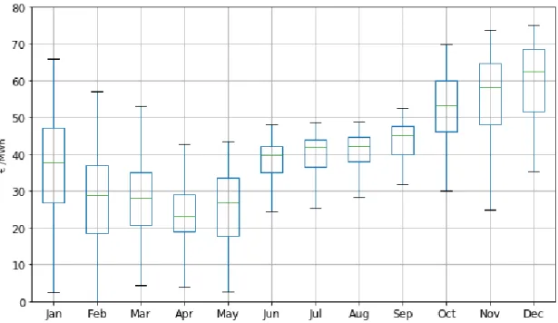
35

Figure 17 - Monthly distribution of Electricity Price during 2016

(45)

36 As can be seen in Figure 16, Figure 17 and Figure 18 prices during colder months (from October to March), tend to have a much higher standard deviation than prices during hotter months (from April to September). This effect is especially noticeable in the year of 2016, where colder months have increased volatility when compared to 2015 and 2017.

Table 2 - Mean, Standard Deviation, Minimum, and Maximum of hotter months

Year Mean Standard Deviation

Minimum Maximum

2015 52.11 10.90 10.00 72.48

2016 35.30 10.43 2.79 58.00

2017 47.78 6.09 26.60 60.15

Table 3 - Mean, Standard Deviation, Minimum, and Maximum of colder months

Year Mean Standard Deviation

Minimum Maximum

2015 48.71 13.25 2.00 85.05

2016 43.57 17.35 0.00 75.00

2017 57.19 13.94 8.00 101.99

From the analysis of Table 2 and Table 3 it is possible to verify in greater detail that as generally found in literature, colder months have a highest average price than hotter months despite not always having the highest average price, as can be seen in 2015 where hotter months had a higher average price than colder months.

Additionally, it seems correct to assume that hotter months present a much more stable price series when compared to colder months, as every standard deviation was smaller in hotter months when compared to their colder counterpart.

Furthermore, in every year studied, the highest and lowest peak of the price series are always present in the coldest months, this naturally results in a higher difficulty in predicting the price series during cold months than hotter months due to the increased volatility shown in the data. This means that seasonality through the year is an extremely

(46)

37 important factor that has a direct and easily identifiable relationship with how and when the price will shift throughout the months and it needs to be taken into account when predicting electricity price series.

Consumption

(47)

38

Figure 20- Correlation between Consumption and Electricity prices

Analyzing Figure 19 it’s clear that the overall shape of the series is about the same as the price series in Figure 12, with the key difference that consumption levels don’t seem to vary at all between each year while prices, especially in 2016, varied a lot. This is probably a good indicator that consumption levels don’t have a strong correlation with the final market price, at least not directly. By analyzing Figure 20 where it can be seen that a low price does not necessarily mean low consumption levels and vice-versa the previous assumption is further confirmed. The correlation between these two variables is 0.47 which is to be expected given the previous explanation.

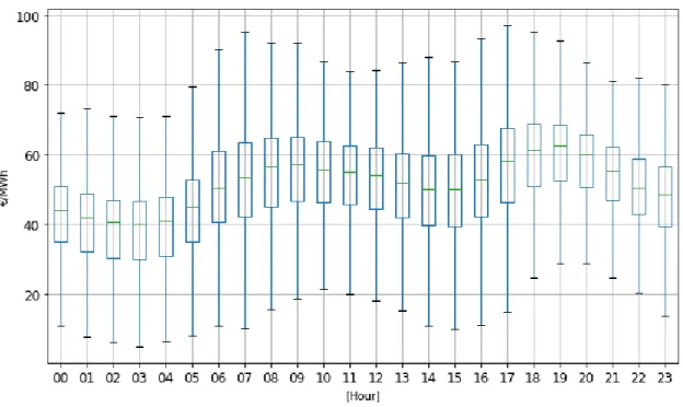
In Figure 21 the hourly distribution can be seen in further detail via a boxplot, and it becomes even clearer that consumption levels present a very strong correlation with the calendar variables, dipping to low levels in morning hours and generally rising to high levels during more active hours.

(48)

39

Figure 22 -Distribution of Consumption from Monday to Sunday

Analyzing Figure 22 the correlation between the period of time and consumption levels becomes even more evident as it follows the exact same pattern as electricity market prices in Figure 12, being stable through the week with not much difference between each work-day and then dropping on the weekends, Sunday being the day where it is at its lowest.

(49)

40

Figure 23 - Daily Average Consumption during hot and cold months

Figure 23 shows the average level of consumption during each year for hot and cold

months, and it is clear that despite the year all consumption levels are extremely similar as long as it’s the same season. This is contrary to the pattern shown by electricity prices, shown in Table 2 and Table 3, where the average price in 2015 during hot months was higher than the average price during cold months, and while there were significant differences between the average price of each year and each season, those differences are not reflected in the consumption levels.

It is clear then that both consumption level and electricity prices are strongly connected to the calendar variables such as the current hour of the day or the weekday but knowing the expected consumption level at a certain hour is not enough to be able to accurately predict the price, as lower consumption levels can still potentially hit high price points and vice-versa. It seems then extremely important to understand the source of the energy that was generated at each point in time and not just the overall energy expended.

Renewable Energy Sources

Hydropower

(50)

41

Figure 25 - Correlation between Energy generated by hydropower and electricity price

(51)

42

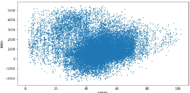
Figure 27 - Correlation between Water Pumping and Electricity Price

Figure 24 represents the added values of hydropower energy generated by hydropower

plants with no reservoirs, reservoirs and mini-hydropower plants, which can generate up to 10 MW/h.

Mini hydropower plants have the lowest contribution to the overall generation, as both reservoirs and hydropower plants generate about 10x more energy each, but it’s still significant enough to include in the data analysis.

Negative energy occurs when plants utilize energy to store water for generating energy at a later time. This usually occurs at night due to prices being cheaper, as can be seen in

Figure 26. This means that a high level of consumption for water pumping is usually

related to cheaper prices. Figure 27 confirms this assumption, as it shows that starting at about the 50€/MWh mark there is much less consumption being utilized for water pumping when compared to lower price points. The lower end of the price range is lot more distributed, meaning that higher levels of water pumping are probably a good indicator to identify when prices are going to be low, as it is likely that water is pumped during periods where price is low.

Water pumping is not however a good predictor for the exact value of price, as for example a consumption level of 0 can be related to any price between 0€/MWh to 100€/MWh.

(52)

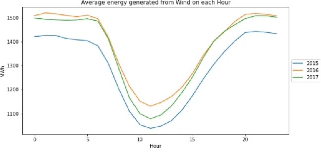
43 The curves in Figure 24 tend to have the same pattern as the consumption curves in

Figure 19 as it would be expected that more energy is generated on peak hours as opposed

to less active hours.

More interestingly, 2016 had a significantly higher hydropower energy generation than both 2015 and 2017 which can partially explain why that year had a significantly lower overall price, as energy from renewable sources is cheaper than fossil fuels. It is still important to note however that electricity prices in 2015 and 2017 are very similar. While 2017 did have the highest average price overall, the difference is not as significant as

Figure 24 would imply, as there is even a point where the average price in 2015 surpasses

2017, which never happens for hydropower energy generation. This means that while hydropower energy generation does seem to have a big impact on the price, it is not the only variable that needs to be considered.

Finally, looking at Figure 25 it’s possible to see that when energy generated from hydraulic sources is at its highest, the price is always in the lower range and at the very low price range, between 0€/MWh and 20€/MWh negative energy almost never occurs which seems to further indicates that high energy generated from hydraulic sources is a good contributor to bringing the final market price down.