A Work Project, presented as part of the requirements for the Award of a Masters Degree in Economics / Finance / Management from the Faculdade de Economia da Universidade Nova de Lisboa.
IMPROVING ACCURACY OF INFLATION FORECASTS USING MACROECONOMIC INFORMATION
ARPAD KOCSIS 2064 / i6093399
A Project carried out on the Master of Financial Economics Double Degree Programme Nova SBE and University Maastricht, with the supervision of:
Francesco Franco and Nalan Bastürk (University Maastricht)
ii
Abstract
This thesis examines the effects of macroeconomic factors on inflation level and volatility in the Euro Area to improve the accuracy of inflation forecasts with econometric modelling. Inflation aggregates for the EU as well as inflation levels of selected countries are analysed, and the difference between these inflation estimates and forecasts are documented. The research proposes alternative models depending on the focus and the scope of inflation forecasts. I find that models with a Generalized AutoRegressive Conditional Heteroskedasticity (GARCH) in mean process have better explanatory power for inflation variance compared to the regular GARCH models. The significant coefficients are different in EU countries in comparison to the aggregate EU-wide forecast of inflation. The presence of more pronounced GARCH components in certain countries with more stressed economies indicates that inflation volatility in these countries are likely to occur as a result of the stressed economy. In addition, other economies in the Euro Area are found to exhibit a relatively stable variance of inflation over time. Therefore, when analysing EU inflation one have to take into consideration the large differences on country level and focus on those one by one.
iii
ABSTRACT II
CHAPTER 1: GENERAL INTRODUCTION 1
INTRODUCTION AND MOTIVATION 1
PERSONAL MOTIVATION 1
ACADEMIC MOTIVATION 2
GRAPH 1:2014–2015YTDEUINFLATION LEVELS (MONTHLY) 4
RESEARCH QUESTIONS 6 CHAPTER 2: THEORY 7 CONTRIBUTION 7 THEORETICAL BACKGROUND 7 CHAPTER 3: METHODOLOGY 9 DATA 9 SOURCE 9
GRAPH 2:1996–2015YTDEUHICP(MONTHLY) 9
TABLE 1:OECDDEFINITIONS:EURO AREA,EU28 10
TABLE 2:OECDDEFINITIONS:MACROECONOMIC VARIABLES 12
GRAPHS 3-10:MACROECONOMIC VARIABLES 15
TABLE 3:REGIONAL STATISTICS PER PERIOD FOR HICP(AFTER LOG TRANSFORMATION) 16
GRAPH 11:EU28HICPLEVELS 1996–2015YTD 16
HICP AS DEPENDENT VARIABLE 16
GRAPH 12:GERMAN INFLATION LEVELS 1996–2015YTD 17
GRAPH 13:HICPEU:LOG DIFFERENCES 20
VARIANCE OF INFLATION 20 TABLE 3:VRTEST 21 METHODOLOGY 22 CHAPTER 4: RESULTS 24 RESEARCH DESIGN 24 RESULTS 26 MEASURES OF EVALUATION 26 REGRESSION OUTPUTS 29
TABLE 4:EUREGRESSION MODELS 31
TABLE 5:MEAN IN GARCH COMPARED 32
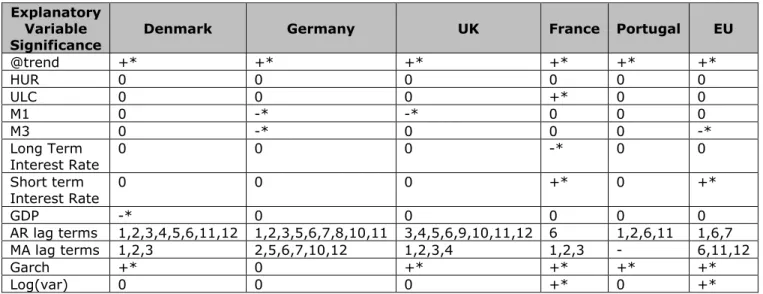
TABLE 6:SIGNIFICANCE OF EXPLANATORY VARIABLES 35
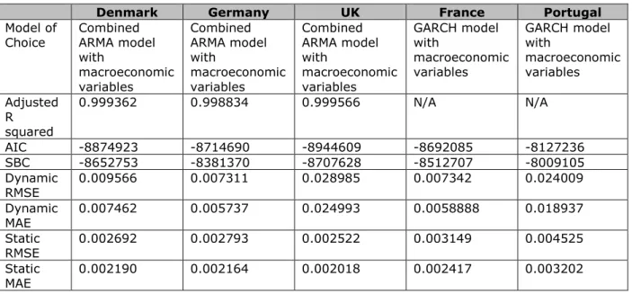
TABLE 7:COUNTRY LEVEL MODELS OF CHOICES 36
ROBUSTNESS CHECKS 37
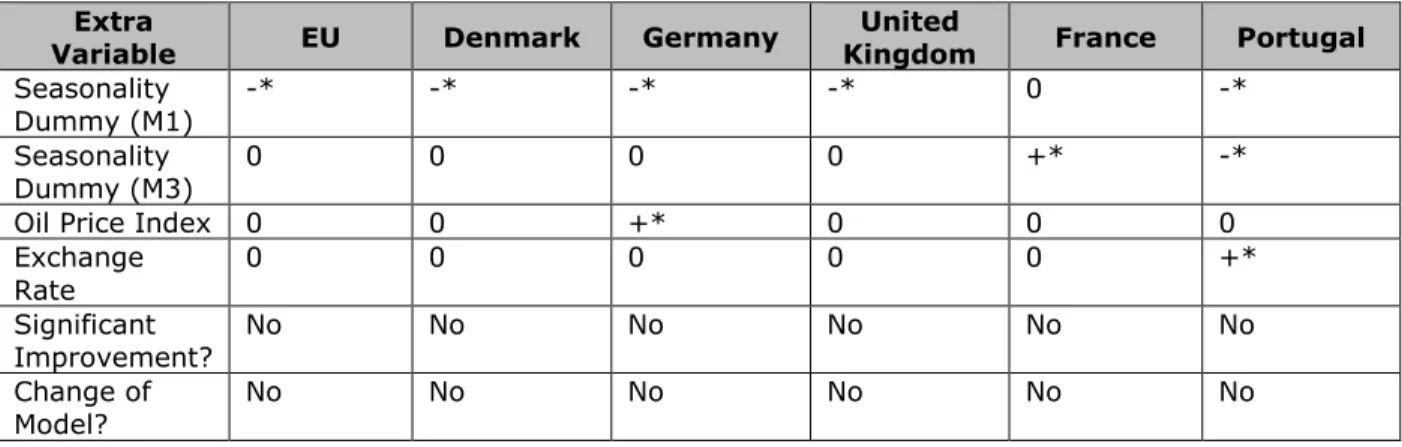
TABLE 8:ROBUSTNESS CHECK 38
iv CHAPTER 5: DISCUSSION 40 IMPLICATIONS 40 FURTHER STUDY 41 CHAPTER 6: CONCLUSION 43 REFERENCES 45
1
Chapter 1: General Introduction
Chapter One introduces general ideas, such as personal and academic motivation. Based on these personal interests, and academic arguments I phrase several research questions.
Introduction and motivation
Personal Motivation
The intention behind the choice of the topic “Improving accuracy of inflation forecasts using macroeconomic information” has been my personal motivation to contribute to the debate about inflation forecasts and their accuracy. The main point of preference for a contribution to this field is my personal interest in econometric modelling and in using statistical tools to forecast future economic movements. A practical application of this amplitude would give me the benefit of a more detailed knowledge of these tools, which have been initially triggered during one of the quantitative courses I took during my studies.
Econometrics deals with complex multivariate relationships between economic data, and econometric applications are mostly based on non-experimental or “field” data that are influenced by many factors. No matter whether we talk about a simple linear regression model or more advanced regression models, most of these classical econometric analyses use some basic assumptions which may be difficult to validate (McFadden in
Robust Methods in Econometrics, 1999). Hence, the interpretation of the results, but also
of the models, has to take into account these difficulties. This is what strikes me the most in the field of econometrics, and this is why I chose a closely related topic.
Furthermore, there are some special issues to be considered when estimating relationships between time series data. Time itself gives a natural flow of the observations which are absent when one uses cross-sectional dataset, and it ultimately leads to dynamic features of the observations. For example, autocorrelation, which is the cross-correlation of a signal with itself at different points in time, or heteroskedasticity especially in the case of autocorrelation raise my interest for different tests, methods, and applications to put in practice.
Putting these econometric methods in practice allows us to estimate different time series models. I find particularly challenging to forecast HICP for the next period in
2
time, and evidently putting the variance of inflation into this context. Besides the application of the different methodologies, the practical contribution of improving the inflation forecasting accuracy can be interesting combined with policy recommendations and it could provide a base for further research in this topic.
Academic Motivation
Inflation itself captures the rate of change of prices, which means the price level today reflects the patterns of past inflation. The rate of inflation over the past year is determined by:
𝐼𝑛𝑓𝑙𝑎𝑡𝑖𝑜𝑛 =
(𝑃−𝑃−1)𝑃−1 (1)
Very high inflation is typically associated with very poor economic performance, with investment, consumption and output being depressed. When inflation is high, it tends to be more volatile and costly simply because it creates an uncertain environment and undermines the informational role of price levels (Carlin, W., & Soskice, D., 2005). On the other hand, if inflation is negative, meaning prices and wages will be lower in a year’s time than they are now, the difficulty of cutting nominal wages raises alongside with the threat of a deflation trap levels (Carlin, W., & Soskice, D., 2005). Consequently, volatile inflation is distortive and masks the relevant changes in the economy causing misallocation of resources.
These arguments about high or negative inflation levels and the uncertainty around them lead to the assumption that if the expectations of the market are meant to be fulfilled, inflation level should be at a close to constant level (Carlin, W., & Soskice, D. (2005).
In the model developed by Carlin, W., & Soskice, D. (2005), we can observe that at higher inflation levels, people want to hold lower money balances, because they wish to economize on their holdings of money, so to restore the equilibrium in the money market, the real money supply must be lower than in the initial low inflation equilibrium (Carlin, W., & Soskice, D. (2005). This leads to additional costs, such as shoe-leather costs (people’s trips to the bank or the cash machines more frequently), and menu costs (the time and effort involved changing price lists more frequently), hence making a higher, more volatile inflation environment considerably more costly (Carlin, W., & Soskice, D. (2005).
3
The book further argues, that policy makers should focus on a nominal anchor for the economy keeping the price level changes (inflation) low and stable. However, we still observe times with high inflation levels and also volatility. Those inflationary problems usually require painful and politically very unpopular solutions, resulting in unresolved social and political conflicts (Carlin, W., & Soskice, D., 2005).
Hence, it is of no surprise that over the past decades, policymakers, central banks, investors and private firms tried to predict the future levels of inflation. They did so because determining how the general price level will change is the key to an informed decision making process (Faust and Wright, 2013). In addition, policy makers use monetary and fiscal policy tools that have effects on inflation. Therefore forecasting HICP is also important to minimize distortions in inflation levels in the economy. However, economic theory often gives a steady state inflation equilibrium, but it is silent about the variation in inflation. Hence it is hard to choose a theory-based model for analyzing inflation variation, this is the motivation to use GARCH models allowing for variance changes over time. The case study by J. Faust and H. Wright examines the different approaches used to forecast HICP in the United States. However, so far only little attention has been dedicated to the actual volatility of the inflation that is the source of uncertainty.
Since the mid-1980s the variability of quarterly inflation has declined by about two thirds, the period known as Great Moderation (Bernanke, 2004). Faust and Wright argue that the presumption that this period will last forever is rather shaky (Faust and Wright, 2013). However, Bernanke remarks that lower volatility of inflation has advantages, such as improved market functioning, easier economic planning, and reduced hedging risks (Bernanke, 2004).
Especially after the recent financial crisis, it is clear that not only the level of inflation, but also its volatility, are of great importance. Determining the main drivers of this inflation volatility and forecasting in this setup would help decision makers to more accurately link future expectations to real levels of inflation. Particularly financial decision makers are interested in inflation and inflation uncertainty since discounts on (expected) future process of assets are directly linked to inflation (and interest rate) expectations.
4
Graph 1: 2014 – 2015YTD EU Inflation Levels (monthly)
The graph above (Graph 1), however, clearly shows that the Euro Area experiences very low levels of inflation since January 2014. The expectation of the European Central bank is that low inflation will be prolonged but gradually return to 2% (Draghi, 2014). The speech by Mario Draghi, President of the ECB, “Monetary policy in a prolonged period of low inflation” at the ECB Forum on Central Banking (Sintra, 26 May 2014) sums up the current developments about low level inflation in the EU:
“…Low inflation is not particular to the Euro Area. Inflation is low across advanced economies, mainly due to the diminishing effect of oil prices on consumer prices. But looking at the anatomy of inflation, there are two factors specific to the Euro Area that contribute to especially low inflation here…”
The first is a common factor: the rise in the euro exchange rate and its effect on the price of internationally traded commodities. The second is a local factor: the process of relative price adjustment in certain Euro Area countries that pulls down aggregate inflation.
Falling commodity prices explain the lion’s share of the disinflation the Euro Area has experienced since the end of 2011. Brent crude oil prices were down by around 7% in euro terms in the first quarter of this year, compared with a year earlier. Food prices were sharply down as well. In fact, these two components have together accounted for
5 around 80% of the decline in Euro Area HICP (Harmonised Index of Consumer Prices) inflation since late 2011.
To add to this, aggregate inflation has been dragged down by local factors linked to the sovereign debt crisis and the process of relative price adjustment in stressed countries. Several Euro Area countries are currently undergoing internal devaluation to regain price competitiveness, both internationally and within the currency union. The crucial adjustments vis-à-vis other Euro Area countries have to take place irrespective of changes in the external value of the euro.
So to sum up: falling energy and food prices, coupled with the effects of relative price adjustment in stressed countries, explain almost fully the disinflation we have seen in the Euro Area…” (Draghi, “Monetary policy in a prolonged period of low inflation” at the
ECB Forum on Central Banking, 26 May 2014)
The European Union and the Euro Area consist of several very diverse economies in different stages. Therefore it is viable to anticipate that the main changes in inflation variance stems from those stressed countries, while other economies as part of the Euro Area (for example, Germany) exhibit a relatively stable variance of inflation over time.
According to these arguments, there is a need of disaggregation to country level analysis and observe how the different country specific trends and macroeconomic variables contribute to the overall inflation levels in the European Union. As Draghi argues, low inflation is not particular to the Euro Area because inflation tends to be low across advanced economies, mainly due to the diminishing effect of oil prices on consumer prices (Draghi, 2014). In those advanced economies, where inflation is low, the stability of the price level changes brings also a more predictable and relatively constant variance over time. So the main question remains, where does the variance change on aggregate level come from and if those more uncertain economies, in fact, are the initial source of inflation variance, how can one incorporate these characteristics into the inflation forecasting model?
6
Research Questions
The research idea focuses on the above-discussed factors and their effects on the inflation levels and inflation volatility in the Euro Area. The central question of the proposed thesis will be:
“Which macroeconomic factors affect the inflation level and its volatility and how?”
More precisely, this research attempts to find an alternative model to determine the levels of inflation in the Euro Area through focusing on its volatility and on the changes of this volatility over time. This leads to several sub questions:
What are the main drivers of volatility changes?
To what extent can these models forecast HICP accurately?
There are several potential macroeconomic factors, such as unemployment or other economic factors used in the USA, which can have an influence on the levels of inflation. Depending on data availability and the models to be used, the above mentioned questions will be addressed and the proposed model based on these variables will be used to answer another set of sub questions:
What is the probability that the volatility of inflation will change in the next period?
How severe will that change be?
What will potentially cause inflation volatility to change?
Are volatility changes accompanied by changes in expected inflation?
What are the similarities and differences in inflation patterns across Euro Area countries?
In order to properly answer these proposed research questions, it is important to take a look at the underlying theories behind these topics.
7
Chapter 2: Theory
Chapter Two outlines the potential contribution of this papers, and introduces the theoretical background of inflation forecasting
Contribution
The academic contribution of this paper would be the focus on inflation volatility together with the levels of inflation. Depending on data availability, other econometric models can also be applied, for example, probit or logit models for predicting the probability of the change in inflation variance. Further, applying a robustness check will ensure that the results can be generalized. Additionally, a case study like the one by J. Faust and H. Wright has not been done in the Euro Area, therefore given good data availability a comprehensive review of used methods can be relevant to European private firms and policy makers. A further contribution is to address similarities and differences in inflation patterns across Euro Area countries.
Finally, most of the research about forecasting HICP has been limited to the USA. Given today’s economy it is timely to look at the Euro Area or some representative countries and provide a study about the inflation volatility in those economies. For example, Rother finds evidence before the financial crisis that the negative consequences of inflation volatility are of particular concern, given the destabilising effects of discretionary fiscal policies (Rother, 2004). So given an even more uncertain time period it is of great importance to examine the main drivers of inflation volatility.
Theoretical background
There has been an extensive amount of research done about inflation and its properties, but the main focus in most studies was the levels of the inflation and the possibility to forecast the future levels of it. To mention a few, whether it is the Phillips-curve model, or market-based inflation hedging methods, the uncertainty component has not been fully encountered. In recent years, macroeconomic forecasting and its uncertainty have gotten more attention, especially after the recent financial crisis. It is also important to mention the probability of deflation (for USA it happened only in 2009 Q3). Without proper estimates of inflation and its volatility, this deflation is an “unexpected” event. This is also a reason for increased attention in the Euro Area to estimating and forecasting
8
volatility. Furthermore, Giordani and Söderlind argue that forecasters underestimate inflation uncertainty (Giordani and Söderlind, 2002).
Hence, forecasting HICP has become the main focus of many studies in the USA and many different approaches have been suggested. For example the model by Stock and Watson (2007), which allows the variances of the permanent and transitory disturbances evolve randomly over time, that is, an unobserved components model with stochastic volatility (UCSV) (Stock and Watson, 2007). Furthermore, Groen et al. (2013) claim that a model allowing for structural breaks in the error variance results in very accurate point and density forecasts (Groen et al., 2013).
Based on these academic articles and supporting theories, it is clear that nowadays many new methods are being used to improve the forecasts of inflation. However, J. Faust and H. Wright argue that a move to a fundamental re-think of the topic of inflation forecasting is called for (Faust and Wright, 2013). Their comprehensive comparison of methods shed light on the performance of these forecasting models in the USA, but on the other side a case study like theirs has not been done in the Euro Area. Although there are a lot of different aspects to consider when forecasting HICP, the attention to its volatility and the sources and main drivers have been avoided in most of these researches. The obvious question now is: “Why did these studies not look at the volatility component?” I plan to answer this question by collecting the most appropriate dataset.
9
Chapter 3: Methodology
DataSource
The major source of data is the ECB’s website, since the Euro Area inflation measures are published there. The exact span of the data is limited for some countries, hence selection of countries and time periods will be based on data availability. Explanatory variables will be macroeconomic factors (such as unemployment, marginal costs) and in addition economic factors from the USA. There are several other potential factors to be included, and these will be decided according to data availability and literature on inflation determinants. As a starting point, I collected the overall Harmonized Index of Consumer Prices (HICP) normalized monthly levels from 1996 (See Graph 2), as well as other potential explanatory variables such as unemployment or labour market productivity. The main source of datasets is OECD’s database.
Graph 2: 1996 – 2015YTD EU HICP (monthly)
Finding a robust and reliable dataset for Europe is a difficult task. The composition of the European Union changed significantly over the past decades, additionally a recent ECB papers argues that:
65 70 75 80 85 90 95 100 105 110 115 Jan -199 6 Au g-1996 Ma r-1997 Oct-199 7 Ma y-1 998 De c-1 998 Ju l-19 99 Fe b -20 00 Se p -20 00 Apr-20 01 N o v-200 1 Ju n -2002 Jan -200 3 Au g-2003 Ma r-2004 Oct-200 4 Ma y-2 005 De c-2 005 Ju l-20 06 Fe b -20 07 Se p -20 07 Ap r-2008 N o v-200 8 Ju n -2009 Jan -201 0 Au g-2010 Ma r-2011 Oct-201 1 Ma y-2 012 De c-2 012 Ju l-20 13 Fe b -20 14 Se p -20 14 Ap r-2015
HICP - EU (2010=100)
10 “…a vast literature has emerged analysing the degree of inflation persistence. One of the central issues is whether inflation persistence follows a unit root. Recent empirical evidence not only suggests inflation has varied over time, but also that inflation is not an intrinsically persistent process…” (Lünnemann, P., and T. Mathä. "How Persistent is Disaggregated Inflation." An Analysis (2004)).
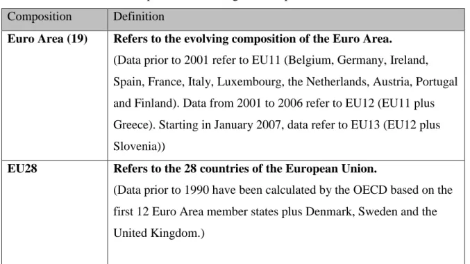
These issues result in some cumbersome dataset issues, which will be explained below after the data description. To correctly interpret the results, the clarification of definitions used by the OECD is needed in order to avoid misconceptions. Table 1 includes the definitions for the compositions referring the European Union:
Composition Definition
Euro Area (19) Refers to the evolving composition of the Euro Area. (Data prior to 2001 refer to EU11 (Belgium, Germany, Ireland, Spain, France, Italy, Luxembourg, the Netherlands, Austria, Portugal and Finland). Data from 2001 to 2006 refer to EU12 (EU11 plus Greece). Starting in January 2007, data refer to EU13 (EU12 plus Slovenia))
EU28 Refers to the 28 countries of the European Union.
(Data prior to 1990 have been calculated by the OECD based on the first 12 Euro Area member states plus Denmark, Sweden and the United Kingdom.)
Table 1: OECD Definitions: Euro Area, EU28
All of the above used definitions, as well as variables inputs are common across all European countries to avoid misconceptions of definitions. Therefore, similar metrics have been used for the analysis. As I mentioned previously, the composition and time span availability of the data differ among variables and also among countries, hence following I list these features of each of the variables. All definitions are taken from the OECD’s database and the wording is kept identical for reliability and validity reasons (See Table 2):
11
Data Frequency Availability Measure Definition by the OECD Database* HICP Monthly For Euro Area and EU
from January, 1996 to August, 2015
Index (2010 = 100)
The Harmonized Index of Consumer Prices (HICP) is the measure of prices used by the Governing Council for the purpose of assessing price stability. Within the European Union, Harmonized Indices of Consumer Prices (HICP) are consumer price indices compiled on the basis of a harmonized coverage and methodology. HICPs at the "all items" level are presented for 21 European countries
Unemployment Monthly For Euro Area from July, 1990 (estimated by ECB) and for EU from January, 2000 to September, 2015 Harmonized unemployment rate: all persons (index), seasonally adjusted
Harmonised unemployment rates define the
unemployed as people of working age who are without work, are available for work, and have taken specific steps to find work. The uniform application of this definition results in estimates of unemployment rates that are more internationally comparable than
estimates based on national definitions of unemployment
Unit Labour Cost
Quarterly For Euro Area from Q1-1996 to Q2-2015
Index (2010 =100), seasonally adjusted
Unit labour costs (ULCs) measure the average cost of labour per unit of output. They are calculated as the ratio of total labour costs to real output. Quarterly ULCs can be decomposed into the components labour compensation per employee and output per person employed (employment-based labour productivity). Every effort has been made to ensure that data are comparable across countries.
M1 Monthly For Euro Area from January 1990, estimated
Seasonally adjusted index based on 2010=100.
Narrow Money (M1) includes currency i.e. banknotes and coins, plus overnight deposits.
M3 Monthly For Euro Area from January, 1990, estimated
Seasonally adjusted index based on 2010=100.
Broad money (M3) includes currency, deposits with an agreed maturity of up to two years, deposits
12
Table 2: OECD Definitions: Macroeconomic Variables
*All definitions are set by the OECD Database. Online at: <https://data.oecd.org/>
repurchase agreements, money market fund shares/units and debt securities up to two years Long term
interest rates
Monthly For Euro Area from January, 1990, estimated to September, 2015
Long-term interest rates, Per cent per annum
Long term (in most cases 10 year) government bonds are the instrument whose yield is used as the
representative ‘interest rate’ for this area. Generally the yield is calculated at the pre-tax level and before deductions for brokerage costs and commissions and is derived from the relationship between the present market value of the bond and that at maturity, taking into account also interest payments paid through to maturity.
Short term interest rates
Monthly For Euro Area from January, 1994 to September, 2015
Short-term interest rates, Per cent per annum
Short term rates are usually either the three month interbank offer rate attaching to loans given and taken amongst banks for any excess or shortage of liquidity over several months or the rate associated with Treasury bills, Certificates of Deposit or comparable instruments, each of three month maturity.
For Euro Area countries the 3-month "European Interbank Offered Rate" is used from the date the country joined the euro.
GDP changes Quarterly For Euro Area from Q2-1995 to Q2-2015 Growth rate compared to previous quarter, seasonally adjusted
Gross domestic product (GDP) at market prices is the expenditure on final goods and services minus
imports: final consumption expenditures, gross capital formation, and exports less imports. "Gross" signifies that no deduction has been made for the depreciation of machinery, buildings and other capital products used in production. "Domestic" means that it is production by the resident institutional units of the country.
13
Based on data availability, and to allow the best fit possible, the data used will be referring the Euro Area from January, 1996 to June, 2015 for all variables. That leaves us with 234 observations for each of the above variables. The small sample size can be a drawback of the analysis. Furthermore, as one can notice, not only the availability and the composition are different, but also the frequency of the datasets differ from each other, therefore I needed to interpolate the GDP changes indicator and the ULC dataset to monthly. This will be a drawback of the analysis further on. Most of the dataset becomes stationary after the first difference, however, the HICP indicator only becomes stationary after the second difference. Possible explanation is seasonality or the existence of change in mean series over time. Standard tests for unit roots then fail and see higher AR coefficients (in the extreme this can lead to a unit root), Maddala and In-Moo Kim point out that although often used, the ADF test is “useless” in practice, because there is no uniformly powerful test for the unit root hypothesis (Maddala, In-Moo Kim, 1999). The aforementioned ECB paper examines this issue more closely and finds out that allowing for a structural break in the series avoids spuriously high inflation persistence estimates. An exogenous break at the start of EMU stage III and the effects of an important modification to the HICP data collection methodology, i.e. the inclusion of sales prices lead to significant mean differences in the date over the analyzed period (Lünnemann, P., and T. Mathä, 2004).
I will follow their methodology to find these structural breaks and include an explanatory variable (such as a dummy variables) to take care of mean changes, then the HICP conditional on this variable will become stationary after the first difference. To formally test, I will run a Chow test for the following breakpoints: 2001Q1 for the inclusion of sales and 1999Q1 for the EMU stage III. To visualize the different types of datasets, and their characteristics, all datasets have been normalized to the 2010 levels, according to the OECD standards. The quarterly data (ULC and GDP) have been interpolated by attributing the quarterly changes equally to each respective month within the quarter (See Graphs 3-10):
14 65 70 75 80 85 90 95 100 105 110 115 Jan -1996 Se p -1996 May-1997 Jan -1998 Se p -1998 May-1999 Jan -2000 Se p -2000 May-2001 Jan -2002 Se p -2002 M ay-20 03 Jan -2004 Se p -2004 May-2005 Jan -2006 Se p -2006 May-2007 Jan -2008 Se p -2008 May-2009 Jan -2010 Se p -2010 May-2011 Jan -20 12 Se p -2012 May-2013 Jan -2014 Se p -2014 May-2015
HICP (2010=100)
HICP_Denmark HICP_France HICP_Germany HICP_Portugal HICP_UK HICP_EU
70 75 80 85 90 95 100 105 110 115 Jan -1996 Se p -1996 May-1997 Jan -1998 Se p -1998 May-1999 Jan -20 00 Se p -2000 May-2001 Jan -2002 Se p -2002 May-2003 Jan -2004 Se p -2004 May-2005 Jan -2006 Se p -2006 May-2007 Jan -2008 Se p -20 08 May-2009 Jan -2010 Se p -2010 May-2011 Jan -2012 Se p -2012 May-2013 Jan -2014 Se p -2014 May-2015
GDP (2010=100)
GDP_Denmark GDP_France GDP_Germany GDP_Portugal GDP_UK GDP_EU
0 50 100 150 200 250 300 Jan -1996 Se p -1996 May-1997 Jan -1998 Se p -1998 May-1999 Jan -20 00 Se p -2000 May-2001 Jan -2002 Se p -2002 May-2003 Jan -2004 Se p -2004 May-2005 Jan -2006 Se p -2006 May-2007 Jan -2008 Se p -20 08 May-2009 Jan -2010 Se p -2010 May-2011 Jan -2012 Se p -2012 May-2013 Jan -2014 Se p -2014 May-2015
Long Term Interest Rates (2010=100)
LT_Denmark LT_France LT_Germany LT_Portugal LT_UK LT_EU 20 220 420 620 820 1020 1220 Jan -1996 Se p -1996 May-1997 Jan -1998 Se p -19 98 May-1999 Jan -2000 Se p -20 00 May-2001 Jan -2002 Se p -2002 May-2003 Jan -2004 Se p -2004 May-2005 Jan -2006 Se p -2006 May-2007 Jan -2008 Se p -2008 May-2009 Jan -2010 Se p -2010 May-2011 Jan -2012 Se p -2012 May-2013 Jan -20 14 Se p -2014 May-2015
Short Term Interest Rates (2010=100)
ST_Denmark ST_France ST_Germany ST_Portugal ST_UK ST_EU
15
Graphs 3-10: Macroeconomic Variables
0 20 40 60 80 100 120 140 Jan -1996 Se p -1996 May-1997 Jan -1998 Se p -1998 May-1999 Jan -2000 Se p -2000 May-2001 Jan -2002 Se p -2002 May-2003 Jan -2004 Se p -2004 M ay-20 05 Jan -2006 Se p -2006 May-2007 Jan -2008 Se p -2008 May-2009 Jan -2010 Se p -2010 May-2011 Jan -2012 Se p -2012 May-2013 Jan -20 14 Se p -2014 May-2015
M1 (2010=100)
M1_Denmark M1_UK M1_EU
M1_Germany M1_France M1_Portugal
20 40 60 80 100 120 140 Jan -1996 Se p -1996 May-1997 Jan -1998 Se p -1998 May-1999 Jan -2000 Se p -2000 May-2001 Jan -2002 Se p -2002 May-2003 Jan -2004 Se p -2004 M ay-20 05 Jan -2006 Se p -2006 May-2007 Jan -2008 Se p -2008 May-2009 Jan -2010 Se p -2010 May-2011 Jan -2012 Se p -2012 May-2013 Jan -20 14 Se p -2014 May-2015
M3 (2010=100)
M3_Denmark M3_UK M3_EU
M3_Germany M3_France M3_Portugal
60 70 80 90 100 110 Jan -1996 Se p -1996 May-1997 Jan -19 98 Se p -1998 May-1999 Jan -2000 Se p -2000 May-2001 Jan -2002 Se p -2002 May-2003 Jan -2004 Se p -2004 May-2005 Jan -2006 Se p -2006 May-2007 Jan -2008 Se p -2008 May-2009 Jan -2010 Se p -20 10 May-2011 Jan -2012 Se p -2012 May-2013 Jan -2014 Se p -2014 May-2015
ULC (2010=100)
ULC_Denmark ULC_France ULC_Germany ULC_Portugal ULC_UK ULC_EU 20 40 60 80 100 120 140 160 180 1 9 17 25 33 41 49 57 65 73 81 89 97 105 113 121 129 137 145 153 161 169 177 185 193 201 209 217 225 233
Harmonized Unemployment Rate (2010=100)
HUR_Denmakr HUR_France HUR_Germany HUR_Portugal HUR_UK HUR_EU
16
Table 3: Regional Statistics per Period for HICP (after log transformation)
Graph 11: EU28 HICP Levels 1996 – 2015YTD
(All data have been normalized to 2010=100 points.)
HICP as dependent variable
Beck et al. (2009) claim that there exist large and long-lasting differences in inflation rates across European regions (see Table 3 and Graph 11), which are not related to business cycle or income growth dynamics (Beck, G. W., Hubrich, K., & Marcellino, M., 2009). They attribute these differences mainly to market distortions and other structural characteristics, which further implies welfare affecting behavior (Beck, G. W., Hubrich, K., & Marcellino, M., 2009). Thus there is a clear motivation to discuss this topic in further detail, from both a forecasting and volatility point of view.
Mean Std Mean Std Mean Std Mean Std Mean Std Mean Std
Denmark 1.96 0.0470 1.89 0.0088 1.89 0.0112 1.96 0.0089 2.00 0.0114 2.02 0.0025 France 1.96 0.0425 1.91 0.0043 1.91 0.0098 1.97 0.0093 2.00 0.0108 2.02 0.0035 Germany 1.97 0.0388 1.92 0.0047 1.92 0.0072 1.97 0.0100 2.00 0.0104 2.03 0.0047 Portugal 1.96 0.0580 1.87 0.0106 1.87 0.0187 1.97 0.0131 2.00 0.0106 2.03 0.0032 United Kingdom 1.96 0.0527 1.90 0.0081 1.90 0.0067 1.95 0.0113 2.00 0.0124 2.04 0.0076 All regions 1.96 0.0487 1.89 0.0069 1.89 0.0112 1.96 0.0111 2.00 0.0106 2.03 0.0043
17
Graph 12: German Inflation Rate 1996 – 2015YTD
(Source:http://www.inflation.eu/inflation-rates/germany/historic-inflation/hicp-inflation-germany.aspx)
When the focus is on inflation levels of a specific country, for example Germany, there are clear changes of dynamics of inflation over the past decade (See Graph 12). These changes in inflation dynamics over time, and across regions call for a closer examination of explanatory variables, not just from an economic point of view, but also from a pure statistical and econometric one. The set of graphs above illustrate the variety of behaviour observed with time series data. In the above section, I paid special attention to stationarity of the variables. Nonstationary variables display a “wandering behaviour”, while a stationary data displays a more “fluctuating” behaviour. The graphs below clearly show that most of the macroeconomic variables I plan to incorporate in my modelling exhibit some sort of “trending” behaviour. The main reason why it is essential to make sure that all data is stationary, prior starting the modelling is that there is a big chance of obtaining significant results from unrelated data when nonstationary time series are used in regression analysis, these are called spurious regressions.
This ties back to my earlier reasoning at the beginning of Chapter 1 about interpretation of the results, since spurious regressions make no sense in reality, although purely on the results, they might well be very significant in terms of numbers and residuals would be highly persistent. Besides nonstationarity, I will also test for cointegration between the below variables. This cointegrating relation is a long run relation. That means that the one series and the other series have a unit root (a stochastic trend), but they don't stray away too far from each other as the error term is stationary. To test this long run equilibrium I will run an Engle-Granger procedure, because when predicting future levels of inflation, one could expect a long run relationship of some variables. Stock and Watson argue here that in general terms, inflation forecasts produced by the Phillips curve are more accurate than using methods
18
based on other macroeconomic variables. However, the forecasts can be improved significantly with measures of real aggregate activity, other than unemployment only (Stock and Watson, 1999). For example, the expectations hypothesis of the term structure of interest rates suggests that the spreads between interest rates of different maturities incorporate forecasts of inflation made by market participants. Similarly, the quantity theory of money predicts that, in the long run, the rate of inflation is determined by the long-run growth rate of monetary aggregates (Stock and Watson, 1999, p305 Forecasting HICP in Journal of Monetary Economics 44 (1999) 293- 335). Their reasoning gives a very good incentive for my choices of variables I plan to use, such as long term and short term interest rates, as well as M1 and M3 levels.
While describing the choice of specific variables I will use, one might ask why HICP is used, especially taking into account its technical difficulties. First, CPI, the other common variable measuring inflation, is not available for Europe, and HICP is more appropriate for the European market. Both the Consumer Price Index (CPI) and the Harmonised Indices of Consumer Prices (HICP) are designed to measure, in index form, the change in the average level of prices paid for consumer goods and services by all private households. Both the CPI and the HICP are used to measure consumer inflation (Central Statistics Office, 2012). There are common similarities in both measures. The purpose of both CPI and HICP is to measure the change in the average level of prices of a fixed basket of consumer goods and services. They both include all private households and foreign tourists on holiday, but exclude institutional households. CPI and HICP use the same price data collected from the same retails outlets/service providers. Compilation and aggregation of both measures are done with the same methodology developed by Eurostat.
However, next to these similarities, there are also a few differences. For example, CPI was first used in the United States already in March 1922, whereas HICP was launched in 1996. The current base reference period of the CPI is 2011, while in the case of HICP is 2010 (as used in the regression analysis later on). The coverage is also different in both cases. The Household Charge was added to the “Miscellaneous goods and services” item heading, however the following item heading are excluded from the HICP’s scope:
Mortgage interest
Building materials
19 House insurance
Union subscriptions
The HICPs enable international comparisons of inflation rates to be made between member states within the European Union. The standardized scope and coverage of the HICP measure makes it a better dependent variable, as those will be similar in all member states of the European Union.
Based on the differences outlined above by the Central Statistics Office, we can conclude that HICP in fact is a better index for inflation due to market properties.
20
Graph 13: HICP EU: Log differences Variance of Inflation
Furthermore, a good motivation for the proposed thesis is that after looking at log differences of the HICP data for Europe, there is a clear difference in the variance of the observed variable (See Graph 13).
To formally test whether there is a statistically significant difference in the variance of the observed variable, one can conduct a VR (Variance Ratio) test. By exploiting the fact that the variance of random walk increments is linear in all sampling intervals, the VR methodology consists of testing the random walk hypothesis against stationary alternatives. This means that the sample variance of k-period return is k times the sample variance of one-period (Charles, A., & Darné, O. (2009)).
The VR at lag k is then defined as the ratio between (1/k)th of the k-period to the variance of the one-period return. To test the hypothesis that a given time series is a collection of independent and identically distributed observations, the central idea of the variance ratio test is based on the observation that when returns are uncorrelated over time, we should have V(k) = 1 (Charles, A., & Darné, O. (2009)).
-0.02 -0.015 -0.01 -0.005 0 0.005 0.01 0.015 0.02 19 96M0 2 19 96M0 9 19 97M0 4 19 97M1 1 19 98M0 6 19 99M0 1 19 99M0 8 20 00M0 3 20 00M1 0 20 01 M0 5 20 01M1 2 20 02M0 7 20 03M0 2 20 03M0 9 20 04M0 4 20 04M1 1 20 05M0 6 20 06M0 1 20 06M0 8 20 07M0 3 20 07 M1 0 20 08M0 5 20 08M1 2 20 09M0 7 20 10M0 2 20 10M0 9 20 11M0 4 20 11M1 1 20 12M0 6 20 13M0 1 20 13M0 8 20 14M0 3 20 14M1 0 20 15M0 5
Log HICP EU
21
Table 3: VR Test
In the case of inflation, it is clear that for any chosen period (k=1,2,….,16) the variance of these subsequence of data is different, hence there is clear variance change over time (See Table 3 above).
Furthermore, this methodology can be further used to indicate high persistency, and consequently a unit root. As discussed in the previous section, high inflation persistence can lead to misinterpreted unit root tests. The measurement of the degree of this persistence is actually another way of testing for unit roots.
As previously discussed, the VR is the variance of the kth difference of a time series by k-times the variance of its first difference (Maddala, In-Moo Kim, 1999), where:
𝑉𝑅
𝑘=
𝑉𝑘𝑉1 (2)
A large econometric literature actually finds that inflation is highly persistent, almost mimicking the behaviour of a random walk process (Altissimo, F., Bilke, L., Levin, A., Mathä, T., & Mojon, B. (2006)). Initially, the motivation behind using the variance ratio test was the paper testing the random walk hypothesis of the Euro exchange rates by Jeng-Hong Chen (2008). Variance ratio test is a powerful tool to test the random walk hypothesis. His work compares three different variance ratio tests and concludes that the Euro/U.S. Dollar exchange rate market is considered weak-form efficient. His results are less relevant to my
Null Hypothesis: LOGHICP is a martingale
Sample: 1996M01 2015M06
Included observations: 232 (after adjustments) Heteroskedasticity robust standard error estimates User-specified lags: 2 4 8 16
Joint Tests Value df Probability
Max |z| (at period 4)* 3.805.108 232 0.0006 Individual Tests
Period Var. Ratio Std. Error z-Statistic Probability 2 0.641223 0.102827 -3.489.123 0.0005 4 0.326548 0.176986 -3.805.108 0.0001 8 0.161048 0.250334 -3.351.337 0.0008 16 0.085799 0.350285 -2.609.874 0.0091 Test Details (Mean = -1.7070694897e-05)
Period Variance Var. Ratio Obs.
1 2.8E-05 -- 232
2 1.8E-05 0.64122 231
4 9.1E-06 0.32655 229
8 4.5E-06 0.16105 225
22
topic, however the methodology he used to interpret the variance ratio tests helps me to understand that there are in fact changes in inflation variance over time. The first graph above clearly shows that variance changes over time, as well as the result of the standard Eviews variance ratio test’s null hypothesis cannot be rejected, hence there is statistical evidence of change in inflation variance over time. These support my initial decision to focus on the variance of inflation as well, and not just on predicting the future levels of inflation itself. Methodology
For determining and examining the effects of macroeconomic factors on inflation and its volatility, I need to determine first which measure of inflation to use. For the decision I will rely on the relevant literature mentioned above to justify my choice between CPI, GDP deflator or other possible measures. To estimate inflation levels and volatility I will use standard inflation (time series) models allowing for mean changes in inflation and variance changes (such as the GARCH model). These models will be extended to include additional explanatory variables for inflation and inflation variance. To identify the changes in inflation and its volatility I will use standard tests, such as the Chow break point test. Since I have to take into account the mean changes I will include dummy variables for this purpose.
There is no ultimate model to forecast HICP, hence I will be modelling different scenarios with different sets of variables and compare these models with the standard GARCH and AR models to test with forecast performance tools which of these models perform better. Since it has been discussed in the previous section, there is a good indication of changes of variance of inflation over time. The ARCH models, where the time varying variance is a function of a constant term plus a term lagged once, the square of the error in the previous period, will be the main starting point of the analysis, which then will be expanded with the macroeconomic variables.
To point out an arguable caveat of inflation forecasting is the argument by Stock and Watson in their paper “Modelling Inflation after the Crisis” (2010). There is a considerable instability in inflation forecasting models, which leads forecasters to use multivariate models. With their extension of their initial time-varying unobserved components model (2007) they hypothesize different scenarios with different predictive variables and conclude that there are
23
several sources of uncertainty within the inflation forecasting models. First, if the volatility of the trend component within inflation varies little then inflation will revert to the trend, however, if the trend itself becomes more volatile then the trend tracks inflation (Stock and Watson, 2010). They also point out that there is a regional component that can change the dynamics of inflation, where the conventional monetary policy becomes ineffective, than most models fails to handle the forecasting.
These difficulties and arguments are compounded and make an even bigger influence in the given European situation, therefore upon review of the most commonly used models for inflation forecasting, I will try to incorporate the best of these methods to improve the accuracy of inflation forecasts.
To sum up this section, Stock and Watson make a very good observation in their other paper “Why has U.S. inflation become harder to forecast” (2007):
Depending on the perspective we take, the rate of price inflation has become both harder and easier to forecast. On the one hand, inflation (along with many other macroeconomic time series) is much less volatile than it was historically, and the root mean squared error of naïve inflation forecasts has declined sharply. In this sense, inflation has become easier to forecast: the risk of inflation forecasts, as measured by mean squared forecast errors (MSFE), has fallen (Stock and Watson, 2007)
On the other hand, if we take univariate models as a benchmark and measure the relative improvement of standard multivariate forecasting models, we find that those models are improving less and less over a naïve forecast of average twelve-month inflation by its average rate over the previous twelve months. In this sense, inflation has become harder to forecast, at least, it has become much more difficult for an inflation forecaster to provide value added beyond a univariate model (Stock and Watson, 2007). These characteristics and new dimensions changed irreversibly the properties of inflation forecasts.
24
Chapter 4: Results
Research DesignAs discussed before, specific properties of inflation and other macroeconomic data need to be analysed prior to the modelling of the inflation forecasting equation. The dependent variable an all analyses of this thesis is the HICP measure (definition and description of these data are provided in Chapter 3). First, to test for stationarity, I employed an Augmented Dickey Fuller (ADF) test. It turns out that the dataset itself might not have a unit root, however, after including the trend in the test, it turned out to be significant and the variable became stationary on the 10% level. To be certain, I also have conducted a Kwiatkowski–Phillips–Schmidt–Shin (KPSS) test also testing for unit root. I continued doing so with all variables on country levels. I have run ADF tests and if a variable showed a unit root I took the log difference and made all variables stationary, if applicable (Results of all stationarity tests are provided in Appendix A).
After transforming all variables to ensure stationarity, I employed standard time series econometric models for stationary data. These models include the Auto-Regressive ( AR) model, Moving Average (MA) model and the combination of the former models, namely ARMA models. Since the dataset is on a monthly basis, I have included 12 lags at first to account for potential (annual) seasonality. Then I have removed the non-significant lags of inflation one by one according to t-tests, thereby improving both the R-squared, and the Akaike info criterion. I have done the same with the macroeconomic variables, using a significance level of 5% in all testss.
To formally test these models capability for forecasting, I have done an in-sample (both dynamic and static) forecasting and compared these models based on their RMSE value and MAE value. I continued doing this until in the given framework the measures of comparison (R-squared, Akaike criterion, MFSE) cannot be further improved. To reach that point, I will need to use more sophisticated models, allowing for mean and variance change over time, such as GARCH models.
Improving inflation forecasting using macroeconomic variables has two purposes. One being to actually forecast HICP, while the other being to judge how the variance of inflation will evolve over time. For the second purpose, including the log of the variance in the
25
equation in the GARCH environment gives a better indication whether the model is able to forecast HICP or the variance of inflation better.
After deciding on an aggregate model for the Euro Area, the following step is to break this framework down to country level analysis. There are certain macroeconomic indicators, and different economy components in each of the Euro Area countries which will help in the understanding of country level differences, as well as to uncover the source of inflation volatility on the Euro Area aggregate level.
Interestingly, on the country level analysis, there are clear differences not just in the significance level of macroeconomic variables, but also whether the GARCH component is significant or not on country level. This means that the overall change of inflation variance stems from country level differences, and those variance changes over time are not present in some countries (GARCH coefficient insignificant). This indicates the diversity of the Euro Area economy and hence makes it harder to forecast HICP properly.
Therefore I follow the steps of the initial Euro Area modelling, and compare the best model and estimation results for each country to the one of the Euro Area. For each country, as well as the Euro Area, the best performing econometric model is chosen according to in-sample fit. This leads us to two models on the Euro Area-wide aggregate level, and one model for each country.
After deciding on the model, I conduct a theoretical “out-of-sample” forecast to judge how well alternative models perform. For this, I divide the dataset into two subsamples. The first period runs from 1996M01 until 2008M06 and the second from 2008M07 until 2015M06. 2008 mid-year is chosen as a breaking point since the start of the financial crisis in the EU affected inflation levels substantially. If the model forecasts are accurate during the crisis period and observed inflation levels lie within the 95% confidence level for inflation forecasts, the model should be robust enough to work well in other periods too.
As institutions have a different focus and approach towards inflation level changes, they will either want to look at dynamic or static forecasting. I will conduct both methods within the same framework for each country.
As a last step, to evaluate the overall performance for the aggregate EU forecast, I also forecast in the model with the rolling window method one period ahead (12 months) and repeat the steps three times for a more complete overview.
26
In the following section, the results are shown with detailed explanation of the evolution of various model choices depending on country and purpose of the model. All unit root test results, regression outputs and forecasting outcome can be found in the Appendix. Results
Measures of evaluation
As explained in the previous section, the final decision of the chosen model will be based on several criteria. Depending on the purpose of the model, and for what it will be used, there are several different ratios and information criteria to compare the models.
The first purpose of the analysis is to explain inflation, hence the models can be compared based on how well the regression fits. For this, the obvious measure is the adjusted R squared. R squared measures the success of the regression in predicting the values of the dependent variable within the sample and is between 0 and 1. The higher the measure the better it fits. However, as ARMA models use many explanatory variables and iterations, the adjusted R squared should be used. This is a close relative of R squared, where the formula corrects for sample size and number of predictors:
𝐴𝑑𝑗𝑢𝑠𝑡𝑒𝑑 𝑅
2= 1 −
(1−𝑅2)(𝑁−1)(𝑁−𝑝−1)
(3)
where p is the number of predictors, and N is the total sample size. However, adding variables to a model always increases R squared and equivalently the likelihood, whereas, information criteria are likelihood based criteria to evaluate / compare model performances. There are two common information criteria: Akaike Information Criterion (AIC) and/or Schwarz Bayesian Criterion (SBC). Both of these measures are founded on information theory. They offer a relative estimate of the information lost when a given model is used to represent the process that generates the data. In doing so, it deals with the trade-off between the goodness of fit of the model and the complexity of the model:
𝐴𝐼𝐶 = −2 ln(𝐿) + 2𝑛 (4)
27
where ln(L) is the maximized value of the log of the likelihood, T is the number of observations and n is the number of explanatory variables in the model. For model selection, the model providing smallest information criteria is preferred. Both of these improve with the likelihood of the model and they penalize for too many parameters in the model (including irrelevant variables will be penalized through n). One advantage of the information criteria is that they are able to compare nested models unlike R squared. For example, AR(1) model is an AR(2) model with parameter restriction β2 = 0:
𝑦𝑡= 𝛽0 + 𝛽1𝑦𝑡−1+ 𝛽2𝑦𝑡−2+ 𝜀𝑡 (6) Although AIC/SBC only provide informal test for model comparison since there is no test statistic or critical value to evaluate the performance of the model. In cases, where AIC will indicate a different model as the better one, I will rely in SBC due to its asymptotic properties.
Another way of evaluating the models is to make a forecast for a historical period. There are two choices of the forecasting methods: dynamic and static forecasting. Dynamic forecasting calculates forecasts for periods after the first period in the sample by using the previously forecasted values of the lagged left-hand variable. These are also called n-step ahead forecasts. Whereas, the static forecasting uses actuals rather than forecasted values, but it can only be used when actual data are available. These are also called 1-step ahead or rolling forecasts.
Furthermore, there are two possible procedures for analyzing or comparing the quality of forecasts: Divide available time series into two subperiods:
in-sample period for estimation of parameters where the period should be long enough to yield well-estimated coefficients;
out-of-sample period (for investigating the quality of the forecasts) where the period should be long enough to have good power when analyzing or comparing the quality of the forecasts.
Then the Mean Absolute Error (MAE) and the Root Mean Square Error (RMSE) are simply given by:
28
𝑀𝐴𝐸 =
∑|𝑒𝑡|𝑛 (7)
𝑅𝑀𝑆𝐸 = √∑
𝑒𝑡2𝑛 (8)
where et = Yt - ft = forecast errors (Yt = actual values; ft = forecast values) and n = number of forecasts. They both measure how close forecasts or predictions are to the eventual outcomes, but the use of RMSE is more common because compared to the MAE, RMSE amplifies and severely punishes large errors.
The last measure to be used in the case of the GARCH model comparisons is the Theil Inequality Coefficient :
𝑈 =
√1
𝑛∑(𝑌𝑡−𝑓𝑡)2
√𝑛1∑ 𝑓𝑡2+√𝑛1∑ 𝑌𝑡2
(9)
If U = 0, Yt = ft for all forecasts and there is a perfect fit. The Theil Inequality Coefficient can be decomposed into three proportions of inequality - bias, variance and covariance. The sum of these three proportions is 1. The interpretation of these three proportions is as follows:
Bias: Indication of systematic error. Whatever the value of U, we would hope that bias is close to 0. A large bias suggests a systematic over or under prediction.
Variance: Indication of the ability of the forecasts to replicate the degree of variability in the forecasted variable.
Covariance: This proportion measures unsystematic error and ideally, this should have the highest proportion of inequality.
From this measure, the change of bias and variance proportions between the simple GARCH and GARCH with log(Var) will be used to evaluate the forecasting power of those models for different purposes.
29
As a last step after evaluating the models based on the above-described measures, we are interested in the forecasting power of the models. One has to take into consideration that the used dataset does not have sufficiently enough number of observations to make a solid split between in-sample and out-of-sample. Therefore, the rolling window method will be used because it performs better due to the structural changes in the estimation period. One has to make the deliberation that the sample is not large enough to get a conclusive outcome only based on the rolling window method.
Regression Outputs
As explained before, the analysis of the forecasting models starts with using the EU aggregate data, and then the chosen model will be modified and/or changed to account for county level differences. The ratios and measures introduced in the previous section will be examined sequentially and the model will be evaluated based on those. In cases where a GARCH model will be used, the R squared will be avoided as those cannot be interpreted in that context.
For modelling purposes I needed to transform all data to stationary data. I did so with the EU HICP by taking the log of all observations and included a “@trend” term to de-trend the data, and by doing so I can reject the ADF test hypothesis (LOG1 (=log(HICP EU) has a unit root) on a 10% significance level. To ensure stationarity I also conducted a KPSS test where the hypothesis is that LOG1 is stationary which cannot be rejected (See Appendix A.1 for the test results). I have repeated the same steps for all macroeconomic variables for both EU and country levels.
After making the necessary transformations for both dependent and explanatory variables, I started with the EU models. The simplest model is an ARMA(1,1) model without any macroeconomic variables (See Appendix B.1). Since the dataset runs on a monthly basis, I have regressed 12 lags from both AR and MA terms separately. Both models (AR(12) and MA(12)) work better than the simple ARMA(1,1), however as the data is highly persistent the results of these models can be further improved by combining the models. By doing so, most of the AR and MA terms become insignificant. Systematically deleting the insignificant AR and MA terms one by one results in Combined ARMA model with AR(1), AR(6), AR(7), MA(6) and MA(12) terms staying significant (See Appendices B.2 – B.4). This represents the
30
seasonality characteristic of inflation and the fact that the inflation expectations usually change over a course of six months.
After deciding on the time series terms to include in the model, I have introduced the macroeconomic variables one by one and keeping the significant ones. This resulted in a model where short-term interest rate and M3 are significant, which is not a surprise since there is a long lasting relationship between those variables and inflation (See Appendix B.5).
So far, all measures and ratios used to evaluate the models have improved with the above models. Although these models have a relatively good forecasting power, we have not yet taken into consideration the variance change over time. Actually one of the underlying assumptions of ARMA models is that variance constant over time, which is clearly not the case (See Chapter 3 page 24). This can be validated through having a Simple GARCH model, where without any macroeconomic variables or further explanatory variables. The Simple GARCH model, where the GARCH term in the Variance Equation is highly significant, performs already better on the basis of AIC and SBC as well as the static RMSE and MAE measures (See Appendix B.6).
The Simple GARCH model can be further corrected with introducing the significant macroeconomic variables. This refines both information criteria measures and forecasting ratios (See Appendix B.7). The results so far are summarized in Table 4 below:
31
Model Equation Adjusted
R-squared
AIC SBC (dynamic RMSE and static)
MAE (dynamic
and static)
ARMA(1,1) log(HICP) = c + @trend + AR(1) + MA(1)
0.998895 -8310474 -8236643 0.009546 / 0.003706
0.007222 / 0.002641 MA(12) log(HICP = c + @trend + MA(1)
+ … + MA(12) 0.999301 -8696461 -8474966 0.009400 / 0.002905 0.007078 / 0.002284 AR(12) log(HICP = c + @trend + AR(1)
+ … + AR(12)
0.999291 -8696937 -8475442 0.011295 / 0.002959
0.009022 / 0.002236 Combined ARMA log(HICP) = c + @trend +AR(1)
+ AR(6) + AR(7) + MA(6) + MA(12) 0.999563 -91725 -905437 0.009007 / 0.002348 0.006284 / 0.001804 Combined ARMA with macroeconomic variables
log(HICP) = c + @trend +AR(1) + AR(6) + AR(7) + MA(1) + MA(6) + MA(11) + MA(12) + log(ST) + log(M3)
0.999577 -9207504 -9028126 0.008543 / 0.006309
0.006309 / 0.001762
Simple GARCH log(HICP) = c + @trend + AR(1) + AR(6) + AR(7) + MA(6) + Ma(11) + MA(12) N/A -9267258 -9104828 0.011437 / 0.002343 0.008467 / 0.001819 GARCH with macroeconomic variables log(HICP) = c + @trend + AR(1) + AR(6) + AR(7) + MA(1) + MA(6) + MA(11) + MA(12) + log(ST) + log(M3)
N/A -9325351 -9131025 0.010159 /
0.002303 0.008081/ 0.001816 GARCH with
log(Var)
log(HICP) = c + AR(1) + AR(6) + AR(7) + MA(1) + MA(6) + Ma(11) + MA(12) + log(GARCH) N/A -9239525 -9047563 0.010398 / 0.001849 0.00787 / 0.001849 GARCH in Mean with log(Var) wth macroeconomic variables
log(HICP) = c + AR(1) + AR(6) + AR(7) + MA(1) + MA(6) + MA(11) + MA(12) +
log(GARCH) + log(ST) + log(M3)
N/A -1567776 -1537535 0.027821* 0.024784*
Table 4: EU Regression Models
*log of non positive number prohibits the static forecasting.
Until now the focus was shifted towards explaining inflation and forecasting within those frameworks. Now we turn to explaining the variance of inflation. This can be done by including the GARCH component in the mean equation as explanatory variable. Since all variables have gone through a log transformation, the GARCH component will be introduced the same way as log(GARCH). This model does perform similarly as the GARCH with macroeconomic variables (See Appendix B.8.1), however, based on the performance of forecasting HICP I select the best performing model as the model without the log(GARCH) component, as it slightly worsens the forecasting power.
32
Although the coefficient of the log(GARCH) component is not significant over the whole sample, it becomes significant when I break the sample into two subsamples. This gives a motivation to further update the model. As a next step I introduced the same significant macroeconomic variables from the GARCH model. This creates a model where the information criteria are almost doubled, and the forecasting evaluation measures are lowered significantly (See Table 4). Still based on purely the forecasting measures the GARCH model with macroeconomic variables is the better one.
On the other hand, the reason of including the GARCH component in the mean equation was to explain the variance of inflation better. Therefore, we turn to the Theil Inequality Coefficient as evaluation measure. The overall coefficient stays approximately stable, but the distribution of the three proportions change when looking at the GARCH model and the GARCH in mean model (See Table 5).
Measure GARCH with macroeconomic variables (dynamic / static) GARCH with log(Var) with macroeconomic variables (dynamic) GARCH with log(Var) (dynamic / static) Theil Inequality Coefficient 0.001124 / 0.000255 0.003070 0.001150 / 0.000260 Bias Proportion 0.000001 / 0.000004 0.793188 0.240211 / 0.018096 Variance Proportion 0.011423 / 0.002220 0.093699 0.000053 / 0.000475 Covariance Proportion 0.988576 / 0.997776 0.113113 0.759736 / 0.981439
Table 5: Mean in GARCH compared
Therefore, depending on the purpose of the forecast one need to judge which model to choose. Between the two GARCH in mean models, the one without macroeconomic variables have a more reliable distribution of the proportions, as the covariance proportions should be the highest of all three. The GARCH in mean model with macroeconomic variables has a very high Bias Proportion, and both RMSE and MAE are lower than the other models.
The results outlined in Figure 18 and 19 indicate that macroeconomic variables do have a powerful impact on forecasting accuracy. As the historical data and the tests and analysis in Chapter 3 showed that there is a clear change in inflation variance over time, the GARCH models are the appropriate models to choose and depending on the purpose of that forecast one has to decide between the GARCH or GARCH in mean equations.
33
After completing the evaluation of the models with information criteria and in-sample forecasting, the final step in the Euro Area-wide modelling is to evaluate the performance of the models with out-of-sample forecasts. Dividing the sample into two periods (For details see Chapter 4 Research Design section) and comparing the forecasted values to the actual ones gives a good indication how well the model performs. The purpose of this is that beyond the coverage of the data there is no way of evaluating the forecasting power of models, therefore treating the second sub-sample as out-of-sample and putting those next to the actual values can help deciding on the forecasting model.
The breaking point is 2008M06, and the period after is treated as out-of-sample. With dynamic forecasting in the GARCH in mean model, the actual inflation levels are within the forecasted 95% confidence interval. That indicates that even in a period where the financial crisis created a very uncertain environment a model allowing for variance change over time and having macroeconomic variables as explanatory variables in the equation the model performs well and its use is realistic (See Appendix C.1.1). We usually are interested in a one-step ahead forecast, as this gives a short-term future outlook for the upcoming period. This can be done with a rolling window forecast. I repeat the same steps as before, but instead of forecasting until 2015M06, I only forecast it until 2009M06 (See Appendix C.1.2). Then I repeat it twice with shifting the in-sample period one-year ahead and forecast with that period again one additional year (See Appendix C.1.3). This results in a more robust forecasting method, and all actual values are within the forecasted 95% interval for all three consecutive rolling window periods. For static forecasting I have followed the same methodology, but in the regular GARCH model, as the log of non positive numbers prevent the one year ahead static forecasting in the GARCH in mean model.
After evaluating and deciding which model to use for forecasting HICP in the Euro Area, we can turn to the country level models. As an initial step, I have regressed the AR(12) and MA(12) models and then combined them together in an ARMA model. Already these results show significant differences to the EU ARMA model, as well as between each country. This indicates that inflation expectations changes have a different pace and intensity over the course of a year in every country making the Euro Area-wide forecasting harder on an aggregate level.