Dissertação para obtenção do Grau de Mestre em Engenharia Biomédica Orientador: Sónia Gonçalves, Professora Auxiliar Convidada, FM-UC Co-orientador: Mário Forjaz Secca, Professor Associado, FCT-UNL

(1)

Licenciatura em Ciências de Engenharia Biomédica

Dependence of IVIM

-

DWI Estimations

on Acquisition Parameters

Dissertação para obtenção do Grau de Mestre em Engenharia Biomédica

Orientador: Sónia Gonçalves, Professora Auxiliar Convidada, FM-UC

Co-orientador: Mário Forjaz Secca, Professor Associado, FCT-UNL

Júri:

Presidente: Prof. Doutora Maria Adelaide de Almeida Pedro de Jesus Arguente: Prof. Doutora Rita Gouveia Nunes

Vogais: Prof. Doutora Sónia Isabel Domingos Marreiros Gonçalves Prof. Doutor Mário António Basto Forjaz Secca

(2)

(3)

(4)

(5)

Page V

Acknowledgements

First, I would like to thank to my supervisor Prof. Sónia Isabel Gonçalves, who offered me the great opportunity of doing my Master Thesis with her in ICNAS and gave me the best support a student could ask.

To Prof. Mário Forjaz Secca for creating the Biomedical Engineering course in our faculty, allowing us to study this subject and be a part of the future.

To Prof. Ruy Costa for all the motivational speeches he gave us in his class, inspiring us to do better and better every single day and to chase our dreams.

To all the friends who shared this journey in Biomedical Engineering on the last 5 years with me. Miriam Cabrita, Valter Fernandes, João Carmo, Rui Pimentel, Luis Alho, Eduardo Pontes, César Rodrigues, Fábio Nascimento, Tiago Oliveira, André Queirós, Alexandre Medina, João Sousa and to everyone else that I’ve shared this life experience that is called University. Special thanks to Miriam Cabrita, who was always there for me and kept with me in the long study nights and to Valter Fernandes who supported and advised me in all the decisions and steps I took in this journey.

To my Erasmus friends, for all the crazy trips in Italy and for letting me know a bit more of their culture, Marius Lhu, David Murphy, Ina Holl, Beatriz Romba, Laura Burgot, Rita Arrais and Kalina Kurstak and all the others that made Pisa the best city in the world.

To everyone in Coimbra, who received me in my Master Thesis experience and made a part of their family, Gil Hilário, Mário Gago, Telmo Neves, Joana Belém, Bruno Correia, José Ribeiro and all the others who showed me why Coimbra is the city of the students.

To all my old school friends who still keep in contact and were always there for me, Diogo Cardoso, André Teixeira, Pedro Cardoso, Vanessa Silva, Gonçalo Mateus, Dário Jesus, Hugo Café, Ricardo Manuel, Gonçalo Vaz, Gonçalo Ribeiro and Ricardo Dias. Special thanks to Ricardo Dias for being the brother that I never had and showing me how great a human being can be.

To the girl who listened and corrected me while I was training my presentation, Rita Real, thank you for all the patience you had and most of all, for helping me relaxing.

Special thanks to Sara Monteiro who was always present on the last two years, advising, supporting and essentially being the best friend someone could have.

Last but not least, to my family, especially to my cousin, my mother who always gave me strength to overcome everything and my father for being the best role model a son could have.

(6)

(7)

Page VII

Resumo

A doença hepática gordurosa não alcoólica (DHGNA) é uma das doenças crónicas do fígado mais comuns no mundo ocidental. Está normalmente associada a distúrbios de saúde como a obesidade, diabetes e a hipertrigliceridemia. Actualmente a biópsia do fígado é a técnica mais utilizada para diagnosticar a DHGNA. No entanto é extremamente invasiva e está associada a uma elevada morbidade e erros de amostragem.

Intravoxel incoherent motion diffusion-weighted imaging (IVIM-DWI) consegue distinguir a difusão puramente molecular do movimento pseudo-aleatório das moléculas de água dentro dos microvasos. A IVIM-DWI tem emergido como uma alternativa possível para a identificação de alterações nos tecidos na DHGNA. No entanto, existem poucos estudos que estudem a dependência dos parâmetros IVIM-DWI dos parâmetros das sequências de aquisição.

Por forma a estudar esta dependência, dois estudos foram feitos: 1) estudo simulativo, onde estudámos a influência dos parametros de aquisição no erro e bias associados aos parâmetros IVIM-DWI; 2) Um estudo In-Vivo que serve de teste à viabilidade das sequências de b-values

obtidas através do estudo simulativo.

Os resultados mostraram que o parâmetro mais afectado pelos parâmetros de aquisição é a pseudo-difusão (D*). Além disso, foi também demonstrado que quanto maior o número de b-values usado, melhor será a estimativa dos parâmetros IVIM-DWI. No entanto, a partir de um determinado número de b-values e para baixa razão sinal-ruído (SNR), o efeito do ruído nos extra b-values contraria o efeito de usar mais b-values. Também foi demonstrado que a sequência de b-values usada para a amostragem, influência bastante as estimativas IVIM-DWI.

Concluímos que a sequência de b-values convencionalmente utilizada não fornece estimativas óptimas relativamente ao IVIM-DWI. Além disso, os resultados demonstram que devem ser atribuídos pesos diferentes a cada parâmetro IVIM-DWI para obter uma melhor estimativa. Também foi observado que a influência do relaxamento T2 deveria ser tomada em conta no modelo Intravoxel Incoherent Motion – Diffusion Weighted Image (IVIM-DWI). Finalmente, o nosso estudo mostrou que na presença de Esteatose, o valor D* decresce significativamente enquanto que D descresce pouco. No entanto, as diferenças entre pacientes com esteatose e saudáveis é extremamente influenciada pelo número de b-values usados, levando a diferentes diagnósticos dependendo desse mesmo número.

(8)

(9)

Page IX

Abstract

Nonalcoholic fatty liver disease (NAFLD) is one of the most common chronic liver conditions in the Western world. It is normally associated with health disorders such as obesity, diabetes and hypertriglyceridemia. The gold standard for the diagnosis and staging of NAFLD is liver biopsy, which is highly invasive and is associated with high morbidity and inherent sampling error.

Intravoxel incoherent motion diffusion-weighted imaging (IVIM-DWI) is able to distinguish between true molecular diffusion and the pseudo-random motion of water molecules inside micro vessels. IVIM-DWI has emerged in the recent years as a possible alternative to probe tissue changes in NAFLD. However few studies have addressed the problem of the dependence of IVIM-DWI parameters on pulse sequence parameters.

In order to study this dependence, two studies were carried-out: 1) A simulation study, where we studied the influence of acquisition parameters on the error and bias associated with IVIM-DWI parameters; 2) In-vivo study in order to test the performance of the b-value sequences derived from the simulation studies.

Results showed that the parameter which is more affected by the acquisition parameters is D*. Furthermore, it was also shown that the higher the number of b-values used to sample the data, the better the estimation of IVIM-DWI parameters is. However, after a certain number of points and for low SNRs, the effect of noise in extra b-values counteracts the effect of having more data points. It was also shown that the b-value sequence that is used to sample the data greatly influences IVIM-DWI estimations.

We concluded that the conventionally used b-value sequence does not provide optimum IVIM-DWI estimations. Furthermore, results show that different weights should be attributed to each IVIM-DWI parameter in order to obtain a better performance of the optimized b-value sequence. Also, it was seen that the influence of T2 relation effects should be accounted for in the IVIM-DWI model. Lastly, our study showed that in the presence of steatosis, the value D* significantly decreased while D only slightly decreased. However, the differences between patients with steatosis and healthy controls were extremely influenced by the number of b-values used, leading to different diagnosis depending on the number of b-b-values used in the acquisition.

(10)

(11)

Page XI

Abbreviations and Symbols

ADC Apparent Diffusion Coefficient

CE-MRI Contrast-Enhanced Magnetic Resonance Imaging

CHB Chronic Hepatitis B

CHC Chronic Hepatitis C

CT Computed Tomography

D Molecular Diffusion

D* Pseudo-diffusion

DTI Diffusion Tensor Imaging

DWI Diffusion Weighted Imaging

EPI Echo-Planar Imaging

ETL Echo Train Length

fMRI Functional Magnetic Resonance Imaging

fp Fraction of Perfusion

HFF Hepatic Fat Fraction

IVIM Intravoxel Incoherent Motion

MRE Magnetic Resonance Elastography

MRI Magnetic Resonance Imaging

MRS Magnetic Resonance Spectroscopy

NAFLD Nonalcoholic fatty liver disease

NASH Nonalcoholic Steatohepatitis

(12)

Gonçalo da Silva Brissos Chimelas Cachola 2013

Page XII

PR Perfusion Rate

RARE Rapid Acquisition with Relaxation Enhancement

S Signal Intensity

SE Single-Echo

SNR Signal-to-Noise Ratio

ss Single-Shot

T2 Spin-Spin Relaxation time

TE Echo Time

(13)

Page XIII

Figure Contents

Figure 1.1 - A diffusion-weighted single-shot spin-echo EPI pulse sequence, where PM is the preparation module and ER is the EPI readout; adapted from [13]. ... 3

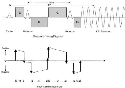
Figure 1.2 - Twice Refocused SE sequence shown as a timing diagram. This sequence allows any diffusion gradient lengths such that the rephasing and dephasing due to the diffusion gradients are equal and TE/2 is the time between the two refocusing pulses. The graph below shows the buildup and decay of eddy currents due to the gradient switching; adapted from [18]. ... 4

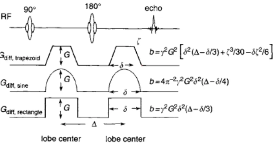
Figure 1.3 - B-values for commonly used diffusion-gradient waveforms in SE pulse sequences; adapted from [13]. ... 5

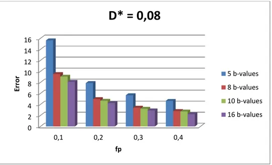
Figure 3.1 - Influence of the number of b-values and fraction of perfusion (fp) in the total error for D*=0,08mm2/s. ... 17

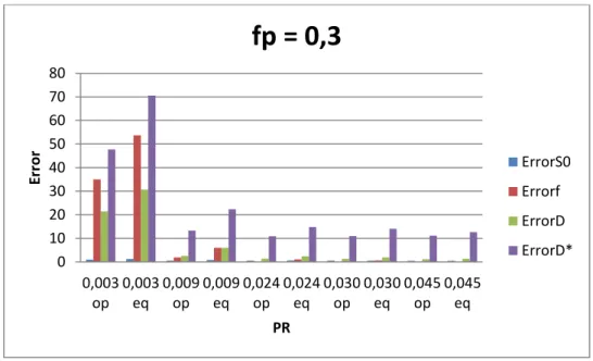
Figure 3.2 - Influence of number of b-values and pseudo diffusion (D*) in total error for fp=0,3. ... 18

Figure 3.3 - Influence of fraction of perfusion (fp) in the relative propagated parameter error for D*=0,08 mm2/s, considering 10 b-values. ... 18

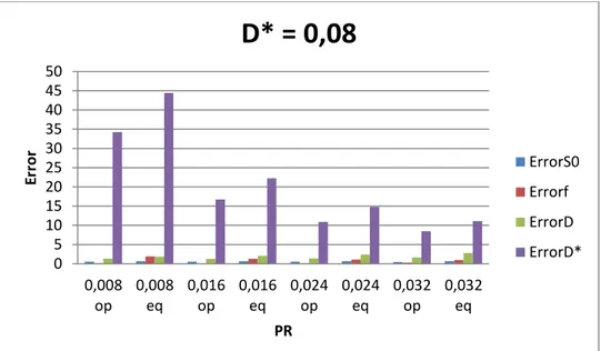
Figure 3.4 - Influence of fp in total error for conventional distribution (eq) and optimum b-value distribution equal weighted (op), considering 10 b-values in both. ... 19

Figure 3.5 - Influence of D* in total error for conventional distribution (eq) and optimum b-value distribution equal weighted (op), considering 10 b-values in both. ... 20

Figure 3.6 - Variation of the relative error of IVIM parameters as a function of PR : A) Constant D*and B) Constant fp, considering 10 b-values in both. ... 21

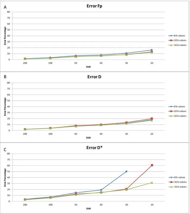
Figure 3.7 - Error percentage for: A) fp, B) D, C) D* ; with 8 (blue), 10 (red) and 16 (green) b-values, for optimum different weighted b-value sequence, fp=0.3 (note: the points not visible in the plot are considered outliers). ... 22

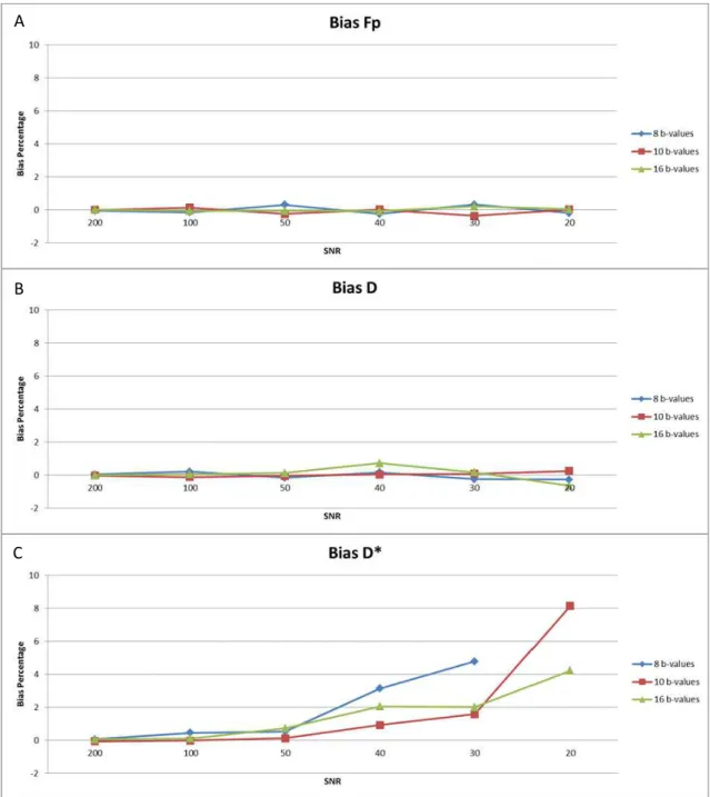
Figure 3.8 - Estimation bias for: A) fp, B) D, C) D*; with 8 (blue), 10 (red) and 16 (green) b-values, for optimum different weighted b-value sequence, fp=0.3 (note: the points not visible in the plot are considered outliers). ... 23

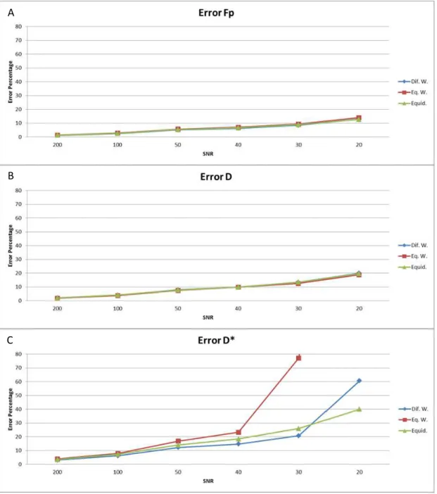
Figure 3.9 - Error for: A) fp, B) D, C) D*, with optimum different-weighted (blue), optimum equal-weighted (red) and conventional (green) b-value sequences, considering 10 b-values and fp=0.3. ... 24

(16)

Page XVI

Figure 3.11 - Estimation error for: A) fp, B) D, C) D*, with optimum different-weighted (blue), optimum equal-weighted (red) and conventional (green) value sequences, considering 10 b-values and fp=0.3. ... 26

Figure 3.12 - Estimation bias for : A) fp, B) D, C) D* with optimum different-weighted (blue), optimum equal-weighted (red) and conventional (green) b-value sequences, for 10 b-values, fp=0.3 and SNR=50. ... 27

Figure 3.13 - Example of the acquired plot for a 16 b-value conventional sequence, for a Control subject. ... 28

Figure 3.14 - Plot of data and model fit for TE= (A) 67ms and (B) 80ms, for subject 1. ... 31

(17)

Page XVII

Table Contents

Table 3.1 - Influence of the number of b-values in in-vivo IVIM-DWI parameter estimation. .. 29

Table 3.2 - Comparison between the Control group and the Patient with Pathology group, regarding IVIM-DWI parameters estimation... 30

Table 3.3 - Influence of TE in IVIM-DWI parameter estimation, for a 10 b-value conventional sequence. ... 31

(18)

(19)

Page 1

1. Introduction

Nonalcoholic fatty liver disease (NAFLD) is one of the most common chronic liver conditions in the Western world [1], progressively becoming a relevant health problem due to the increasing predominance of obesity in the world [2]. NAFLD is normally associated with health disorders such as obesity, diabetes and hypertriglyceridemia, and it is often coupled with increased production of hepatic enzymes [2].

NAFLD has four main stages of increasing severity: simple fatty liver, also known as Steatosis, Non-Alcoholic Steatohepatitis (NASH), Fibrosis and Cirrhosis [3]. Steatosis is the first stage of NAFLD and it is characterized by the excessive accumulation of fat inside the hepatocytes. It is a condition that is generally considered to be harmless, and though it does not normally have associated symptoms, it can be detected with blood tests. NASH is the second stage in NAFLD, being more aggressive than simple steatosis. Only a minor percentage of people [4] with steatosis develop NASH, which contrary to steatosis shows liver tissue inflammation in addition to fat accumulation. Fibrosis is characterized by a persistent inflammation of liver parenchyma, which results in the generation of fibrotic scar tissue around the liver cells and blood vessels. Cirrhosis is the most severe stage when scar tissue and liver cells start to develop, causing liver irregularities as well as a decrease in its size. The damage caused by Cirrhosis is permanent and cannot be reversed; it progresses slowly and may lead to liver failure. Being actually possible to diagnose NAFLD, an important step to take is to determine its stage, which would provide relevant information on prognosis [3].

Percutaneous liver biopsy is considered to be the gold standard for the diagnosis and staging [5] of NAFLD. However, liver biopsy is an invasive technique with potential risks [5], expensive, inherently prone to bias due to limited tissue sampling, and difficult to repeat [6]. This implies that the use of an alternative, non-invasive and reproducible technique for NAFLD diagnosis and staging is essential [5]. Imaging methods such as Transient Elastography [TE] using ultra-sound or dynamic Computed Tomography (CT) have been used as possible alternatives to liver biopsy in the diagnosis and staging of NAFLD. With TE, it is possible to quantify the elastic properties of tissues [7] and it has been used to evaluate liver stiffness [6, 7, 8]. Results show that the latter has a large correlation with the stages of liver fibrosis in patients with chronic hepatitis B or C [7, 8] (CHB, CHC). Dynamic CT in association with compartmental models has been used to quantify liver perfusion [10].

(20)

Page 2

frequency variations of spins related to the chemical environment where they are inserted. It is used to non-invasively quantify the amount of several biological molecules that are involved in both pathological and non-pathological processes. In CE-MRI, a contrast agent is injected in the blood and the temporal variation of its uptake by the tissues is studied [12] using fast imaging pulse sequences whereas in DW-MRI, image contrast is sensitive to the diffusion of water molecules [13]. Recent studies [14] have shown that both CE-MRI and DWI provide potential markers for fibrosis and cirrhosis. Magnetic Resonance Elastography (MRE) is another non-invasive imaging method that can be used to stage NAFLD [15]. It measures the stiffness of soft tissues by introducing shear waves and imaging their propagation using MRI. Huwart et al. [15] showed that MRE is superior to Ultrasound Elastography (UE) and is a reproducible method that has been applied in NAFLD [14].

1.1 Diffusion-weighted imaging

1.1.1 Molecular Diffusion

Diffusion is essentially the thermal random motion of molecules in a medium at temperatures above absolute zero and it is a function of temperature, viscosity and particle size. The Einstein equation [13] describes the behaviour of unrestricted diffusion according to:

√

Where rrms is the one dimensional root-mean-squared particle displacement, t is the diffusion time and D is the diffusion coefficient (mm2/s).

In tissues, the diffusion of water molecules is not unrestricted, but it is rather affected by the constraining presence of macromolecules and other cellular (subcellular) structures. Generally, diffusion in tissues is anisotropic, since the existent restrictions do not have spherical symmetry. The directional dependence of the diffusion coefficient can be described by a 33 matrix, known as diffusion tensor:

[

]

(21)

Page 3

1.1.2 Imaging

Carr and Purcell [17] observed that in the presence of a magnetic field gradient, the diffusion of water molecules causes phase dispersion of the average transverse magnetization of the sample, which causes MR signal attenuation. In DWI, image contrast is sensitized to diffusion through the introduction of strong diffusion-weighting gradients prior to the imaging acquisition module. These gradients are used to increase the sensitivity of pulse sequences to molecular motion due to diffusion. An inherent problem to DWI is that by introducing diffusion gradients, the pulse sequence also becomes more sensitive to other types of motion (e.g. bulk motion), which can cause severe image artifacts that are difficult to correct. In order to prevent this, single-shot pulse sequences, such as single-shot echo-planar imaging (ss-EPI), RARE (Rapid acquisition with relaxation enhancement), or spirals are commonly used [13].

Single-shot SE-EPI (ssSE-EPI) (fig. 1.2) is the most commonly used sequence for diffusion imaging because it is very fast and insensitive to motion. In the conventional implementation of this pulse sequence, the EPI readout follows the diffusion SE preparation module which consists of a 90 excitation pulse followed by a 180 refocusing pulse. The diffusion gradients are positioned on both sides of the 180 pulse and are usually played at the maximum amplitude that is allowed by the hardware.

Figure 1.1 - A diffusion-weighted single-shot spin-echo EPI pulse sequence, where PM is the preparation module and ER is the EPI readout; adapted from [13].

(22)

Page 4

(ETL) in the EPI readout. A smaller ETL reduces the amount of time that off-resonance spins have to accumulate phase errors, thus minimizing image geometric distortions.

The fact that SE-EPI combines atypically large Eddy currents, caused by the large amplitude diffusion-weighting gradients, with an eddy current-sensitive EPI readout, also contributes to image spatial distortion, which is dependent on the direction of the applied diffusion gradient [18]. A commonly used method to overcome this problem is the one introduced by Reese et al [18], which is based on employing twice-refocused RF spin echoes with two bipolar diffusion gradient pairs to more efficiently cancel the Eddy currents (fig. 1.3).

Figure 1.2 - Twice Refocused SE sequence shown as a timing diagram. This sequence allows any diffusion gradient lengths such that the rephasing and dephasing due to the diffusion gradients are

equal and TE/2 is the time between the two refocusing pulses. The graph below shows the buildup and decay of eddy currents due to the gradient switching; adapted from [18].

In an ideal sequence, where the RF pulse durations and gradient ramping times are infinitely short, the timing constants in fig. 1.2 are related according to:

where TE is the echo time, δ1+ δ2 and δ3+ δ4 are the lengths of the two bipolar field gradients, tpr is the sum of the preparation time following the excitation pulse and the readout time preceding the SE. As we have four unknowns and three equations, one of the gradient lengths

(23)

Page 5

refocusing pulse. Furthermore, if the Eddy current decay time constant is known, gradient lengths can be calculated so that Eddy current build-up is nulled prior to readout.

Diffusion weighting in DWI increases with b-value, which depends not only on the amplitude and shape of the diffusion gradients but also on their duration and timing. The b-value is related to the diffusion-weighting gradient waveform ⃗ by:

∫ [∫ ]

where  is the gyromagnetic ratio and t is time

Figure 1.3 shows the explicit dependence of b on gradient parameters for commonly used diffusion-gradient waveforms in SE-EPI sequences.

Figure 1.3 - b-values for commonly used diffusion-gradient waveforms in SE pulse sequences; adapted from [13].

(24)

Page 6

1.1.3 Signal modelling

In the presence of a gradient, molecular diffusion attenuates the MR signal according to:

where S and S0 are the voxel signal intensities with and without diffusion weighting respectively, D is the diffusion coefficient and b is the b-value.

Contrary to what happens in DTI, the approach in (1.3) does not take the directional dependence of D into account. However, the contrast of a DW image can change due to patient orientation. In order to remove this spatial dependence from the image contrast, three DW images, corresponding to diffusion gradients applied along three orthogonal directions, can be used. If Sx, Sy and Sz are signal intensities measured in each of the three images, then the following relations hold:

Where bxx, byy, and bzz are the b-values associated with each of the diffusion gradient directions. If the same b-value is used in all three directions, the geometric mean of the signals is:

√

_⁄

⁄

Where Dtrace is the sum of the diagonal elements of the matrix in Eq. (1.2). The trace is rotationally invariant, i.e. it has exactly the same value independently of the rotation applied to the coordinate system, which implies that Sxyz is independent of the patient orientation.

In practice, signal attenuation in DWI is due to molecular diffusion and perfusion. The origin of the perfusion effect in signal attenuation lies in the movement of spins within randomly oriented capillaries, which mimics a pseudo-diffusion motion. The mathematical formalism describing both effects in signal attenuation is explained in section 2.1.

1.2 The clinical application of Intravoxel Incoherent Motion

–

Diffusion Weighted Imaging (IVIM-DWI) in NAFLD

–

Literature review

(25)

Page 7

Diffusion Coefficient (ADC). This coefficient is said to be apparent because it does not only measure the effect of molecular diffusion in tissues, but also the effect of the pseudo-diffusion in the capillary network within these tissues. Therefore, the signal variation that is measured from tissues with DWI as a function of b is better described by a bi-exponential model, which contains both the contributions from molecular diffusion (D) and pseudo-diffusion (D*) due to perfusion [19]. If for brain tissues, where the fraction of perfusion is low (<4%) [20], the mono-exponential model is a good approximation, that is not the case for e.g. the liver, where the fraction of perfusion in the tissue is approximately 30% [21].

Intravoxel incoherent motion (IVIM) imaging is a method to quantitatively evaluate the microscopic translational motion that occurs in each image voxel [22]. In IVIM-DWI, images are acquired at multiple b-values and it has been shown [22] that it is capable of distinguishing D from D*. The relation between signal variation and b-values in the context of IVIM was described by Le Bihan [19] as:

where Sb is the signal intensity for a given b-value, S0 is the signal intensity for b equal to zero, fp is the fraction of perfusion, D is the pure molecular diffusion (slow component), and D* is the pseudo-diffusion, or fast component [22].

Several studies have tried to show the clinical application of IVIM-DWI to liver imaging [4, 19, 20]. In [22] IVIM-DWI using 10 b-values was applied in the calculation of diffusion parameters in patients with cirrhosis. It was concluded that both D* and ADC are significantly reduced in cirrhotic patients when compared to healthy controls, while fp and D were similar in both groups. This appears to imply that in cirrhotic livers changes in liver architecture are of less importance when compared to changes in liver perfusion. However, the conclusions in [5] point in a slightly different direction. Here IVIM-DWI analysis was applied to an animal model of cirrhosis and results showed that in cirrhotic livers, both D* and D were decreased when compared to healthy liver. Contrary to [22], this suggests that both molecular diffusion and perfusion contribute to the changes in ADC observed in cirrhotic livers.

Patel et al. [6] studied the use of IVIM DW-MRI and DCE-MRI alone and in combination for the diagnosis of liver cirrhosis. Their study suggested that all diffusion parameters (ADC, D*, D, f) were significantly reduced in the cirrhotic group when compared to the non-cirrhotic group. Although DCE-MRI results showed that both portal venous flow and total liver flow were decreased in cirrhosis, a significant correlation between CE-MRI and IVIM-DWI parameters was not found.

(26)

Page 8

ADC on DWI. The inverse correlation between HFF and ADC could be explained by the fact that increasing fat content of liver cells and extracellular fat accumulation would lead to reduced interstitial space and consequent increased restriction to water diffusion, resulting in lower ADCs. Guiu et al. [23], used IVIM DWI to study the difference between D, D* and fp in patients with type 2 diabetes with and without liver steatosis. Results showed that while D and D* are significantly decreased in steatotic when compared to non-steatotic livers, fp shows the opposite behaviour. It is suggested that the presence of large fat droplets in the cytoplasm of hepatocytes causes the displacement of the remaining contents of the cell peripherally, which leads to the decreased mobility of water molecules in the extra-cellular environment. In addition, the decrease in D* indicates that this structural change is associated with decreased parenchymal perfusion. Finally, the increase in fp is probably due to the shorter T2 of the tissue compartment signal, when compared to that of the vascular compartment, which causes an overestimation of the signal fraction of the vascular compartment [17, 20].

1.3 Optimal b-value distribution

The importance of the choice of b-value distribution for IVIM-DWI data acquisition on parameter estimation has been stressed by several authors. In [20], Lemke et al. suggested that for an optimal estimation of the diffusion coefficient, additional higher b-values should be used, since their study only had one b-value higher than 200 s/mm2. In [6], Patel et al. attributed the absence of differences between normal and cirrhotic livers using IVIM parameters, obtained in previous studies, to the limited number of b-values used, especially below 200 s/mm2. Chandarana et al. [21], stated that there is no actual consensus about which b-values are optimal for liver imaging, and that their choice was completely arbitrary and based on the investigator’s experience and type of protocol. Zhang et al. [24], pointed that one of the key points of the IVIM model was the selection of proper b-values in order to provide maximum precision of diffusion parameters. Finally, Lemke et al. [20] evaluated the extent to which the bi-exponential signal decay could be attributed to the vascular compartment. Their study verified that the signal decay in IVIM-DWI of the pancreas in human in-vivo experiments was strongly influenced by the vascular component (fraction of perfusion>11%). Furthermore, it was observed that there was a significant increase of the fraction of perfusion with TE whereas the same type of dependence could not be observed in D and D*. It is suggested that this dependence is artificially created by the large difference between the T2 relaxation times of blood (T2=290 ms @ 1.5T) and (pancreatic) tissue (T2=46 ms @ 1.5T). In this situation, the signal drop in the lower b-value range is larger for the short than for the long T2 species, which leads to an overestimation of the fraction of perfusion. This dependence disappears when the T2 relaxation effects are taken into account in the computation of fp, D and D*.

(27)

Page 9

effects of b-value distribution on IVIM parameter estimation. In the studies of Lemke et al. [25] and Zhang et al. [24], two different methods have been respectively proposed to tackle the problem of selecting the optimal b-value distribution to decrease the errors of IVIM-DWI estimations. In [25], the optimal b-value distribution is obtained through Monte Carlo Simulations. In this method, optimum b-value distribution is searched by consecutively adding new b-values to the b-value sequence, performing Monte Carlo Simulations in each iteration in order to compute the relative errors of each IVIM parameter as:

( √ ∑ ) ( √ ∑ ) ( √ ∑ )

And the relative overall error is:

where, fpi, Di and Di* are the fitted results of the ith repetition and fp, D and D* the values of the selected parameter set. The values, fp, D and D* are used to calculate the individual relatives errors instead. The optimal b-value distribution is selected by choosing the one that minimizes the overall error in 1.10. The main limitation of this method is that it is not certain that the obtained b-values are optimal for any number of b-values.

In [24], the optimal b-value distribution is calculated through the minimization, in a least squares sense, of an error propagation factor. This study considered that in the process of model fitting, random noise in the DWI signal would propagate into the estimate of the model parameters. It assumes that given a set of biexponential parameters and a set of b-values, an error propagation factor for each IVIM model parameter could be predicted (mathematically explained in section 2.1.2). Furthermore, it assumes that each parameter may contribute differently to the total propagated error.

(28)

(29)

Page 11

2. Materials and Methods

1

2.1 Optimization of b-value distribution through the minimization

of an error propagation factor

Considering equation (1.8), since D* is approximately two orders of magnitude greater than D, its influence can be neglected for b-values higher than 200 sec/mm2 [5] and D can be straightforwardly computed by a linear fit to the following expression:

Once D is known, fp and D* can be computed by performing a non-linear fit of the data to (1.8), in a least-squares sense, using the Levenberg-Marquardt method [24] and the cost function R’(fp, D, D*):

∑( )

Where S’i and S’i,Data are the normalized signal intensities, computed as in (1.8) and measured experimentally (for b=bi) respectively.

The calculation of D, D* and fp in two-steps greatly simplifies the computations, in particular because the number of non-linear parameters to be calculated from (1.8) reduces from three to two.

In [24], it is noted that given a set of DWI measurements at multiple b-values bi, parameters, fp, D*, D, can be determined, in a least-squares sense by minimizing the sum of squared residues between the data and the model fit R(S0, fp, D, D

* ):

∑

where Nb is the total number of b-values and Sbi is the signal measured at bi. In order to minimize (2.3), partial derivatives with respect to S0, fp, D, and D

*

have to be nulled:

∑ { [ ] } 1

(30)

Page 12 where x(m) (m = 1, 2, 3, 4) represent S0, fp, D, and D *

, respectively.

After mathematical manipulations (see Appendix A), an error propagation factor ξ can be defined as the ratio of the relative error in a model parameter to the relative input noise δ/S0:

_⁄⁄ √ ∑ ∑ [ ∑ ( ) ]

Where  is the noise standard deviation, x(n) represent S0, fp, D, and D *

and x(n) is the column vector of estimation errors for each parameter and n runs over the number of parameters, four in this case. The elements of A-1 and the partial derivatives S/x are defined as in Appendix A.

In order to calculate the total error that is propagated into IVIM-DWI parameters, the errors of D, D* and fp are summed:

Where Wfp, WD* and WD are the weights associated with the error propagated into fp, D* and D respectively. The calculation of the optimum b-value distribution to estimate a given set of parameters D, D* and fp is performed by means of minimizing (2.5) with respect to bi using the Levenberg-Marquardt method.

In practice, the IVIM-DWI signal consists of the contribution of tissues with different native D, D* and fp values. Therefore, a natural extension of (2.6) is to consider the

contribution of various tissues to the total error - ̅

̅ ∫ ∫ ∫

where Xmax and Xmin are the expected range values of each parameter.

2.2 Simulation studies

(31)

Page 13

phase, the performance of each of the b-value distributions in estimating IVIM-DWI parameters was tested against the presence of noise through Monte Carlo simulations.

In all simulations, the Levenberg-Marquardt [24] minimization algorithm was used to minimize the total propagated error (detailed in section 2.1.2) into IVIM-DWI parameters. The minimization would stop if the number of iterations exceeded 800 or if the variation of the cost function from iteration to iteration would be smaller than 1e-6. In order to avoid local minima of the cost function, the Levenberg-Marquardt algorithm was always applied to a set of twelve or thirteen different starting b-value sequences, finding then the distribution with the minimum overall propagated error, considering this the optimal b value distribution.

In the first phase of the study, the dependence of the propagated error on Nb, TE, T2, fp, D* and PR was investigated in three steps:

1) The influence of D*, fp and Nb on the propagated error of IVIM-DWI estimations was investigated. For that, the optimal b-value sequence with equal weights was used to calculate the total and partial errors propagated to D, D* and fp. The number of b-values Nb, fp and D* were varied according to Nb=5, 8, 10 and 16, fp=0.1, 0.2, 0.3 and 0.4 and D*=0.01, 0.03, 0.08, 0.10 and 0.15. Further simulation parameters were T2=34 ms [22], D=0.00123 mm2/s [22], S0 =100, and considering no transverse relaxation effects.

2) The influence of b-value distribution on the propagated error of IVIM-DWI estimations was investigated. The same simulation parameters of the previous step were used, using optimum b-value sequence with equal weights and conventional sequence and comparing results obtained with each.

3) The influence of PR variation on the propagated error of IVIM-DWI estimations was investigated. For that, the same simulation parameters were used and PR was varied in a fixed interval in two different ways. In the first situation, PR was varied by changing D*, while keeping fp fixed (=0.3), whereas in the second situation the reciprocal was considered (D*=0.08 mm2/s). Parameter PR was varied according to PR=0.003, 0.006, 0.009, 0.012, 0.015, 0.018, 0.021, 0.024, 0.027, 0.030, 0.033, 0.036, 0.039, 0.042 and 0.045.

In a second phase, the performance of each of the b-value distributions in estimating IVIM-DWI parameters was tested against the presence of noise through the performance of Monte Carlo simulations (detailed in section 1.3), using three types of b-value combinations, derived from the first set of simulations:

- Conventional sequence: the b-values are chosen as used in conventional clinical applications (e.g. 0 5 15 30 40 80 100 200 400 800 s/mm2);

(32)

Page 14

- Optimum b-value sequence with different weights: the b-values are obtained as in

Optimum b-value sequence with equal weights, but considering that Wf≠WD*≠WD.

Here, the propagated error was calculated not for one specific D* but for a range of D* values in the interval ranging from 0.01 to 0.15 using 2.7. The weights WD, WD* and Wf were extracted from step three of the first phase of the study by fitting the lowest (possible) order polynomial to the data. Bias and Error presented in all results were calculated as explained in section 1.3. This phase was performed in two steps:

1) The influence of b-value distribution, noise and T2 relaxation effects on Bias and Error of IVIM-DWI estimations was investigated. For that, the three types of b-value sequences were used to calculate the Error and Bias of D, D* and fp. The number of b-values Nb and fp were 10 and 0.3, respectively. Further simulation parameters were T2=34 ms, D=0.00123 mm2/s (liver parameters) measured at 3T [22], S0 =100. Firstly, in order to study noise influence, SNR was varied according to SNR=200, 100, 50, 40, 30 and 20 and relaxation effects were not included. Secondly, to study the influence of T2 relaxation effects, TE was varied according to TE=50, 60, 70, 80, 90 and 100ms and SNR was kept constant at 50.

2) The influence of the number of b-values on Bias and Error of IVIM-DWI estimations was investigated. For that, Nb=8, 10 and 16 were used to calculate the Error and Bias of D, D* and fp. Optimal b-value sequence with different weights and considering fp=0.3 were used. Further simulation parameters were the same as before and relaxation effects were not included.

2.3 In-vivo studies

The influence of TE and b-value sequence on IVIM-DWI estimations was investigated in in-vivo studies that were divided in two phases. First, the dependence of IVIM-DWI estimations on the number of b-values used to sample the signal (Nb) was investigated in data that had been previously acquired in the framework of a running project. The clinical population consisted of 34 diabetes type II patients (21 females and 13 males with mean age 60±8) and 40 controls (25 females and 15 males with mean age 49±7) and all gave written informed consent. The patient group consisted of men and women with type II diabetes, diagnosed at least 1 year prior, age 40-74 years. The control group was age matched to the patient group and without a history of neuropsychiatric, renal, liver, heart, ocular or any other severe non-age related disease, not related to diabetes. A sub-group of 10 patients having Steatosis was created.

(33)

Page 15

mm in-plane resolution, 1 slice 10 mm thick, TR/TE=3800/67 ms, parallel imaging factor 2, 3 or 5 averages using the 4- or 16-channel coil respectively, 16 b-values (0, 5, 10, 15, 20, 25, 30, 35, 40, 50, 70, 90, 100, 200, 400, 800). IVIM-DWI estimations using these data were recomputed with 8 (0, 20, 40, 80, 100, 200, 400, 800) and 10 (0, 5, 15, 30, 40, 80, 100, 200, 400, 800) b-values, and compared with the original estimations that were obtained with 16 b-values.

In a second phase, the performance of each of the b-value distributions, conventional sequence, optimum b-value sequence with equal weights and optimum b-value sequence with different weights, as well as the influence of T2 relaxation effects in estimating IVIM-DWI parameters was tested in healthy volunteers. Eight healthy volunteers (4 females and 4 males, mean age 22±1) were enrolled and gave written informed consent. This volunteers were separated in two groups, one to study the influence of T2 relaxation effects with 2 volunteers (2 females, with 22 and 24 years old), and the other one to study the performance of each b-value distribution (2 females, 4 males, mean age of 22±1).

On the first group, magnetic resonance liver imaging was performed on a whole body 3T imaging system (Magnetom Trio Tim, Siemens Medical Solutions, Erlangen, Germany) using a 16-channel body coil. Respiratory triggered IVIM imaging was acquired using conventional SE-EPI with acquisition parameters: FOV= 300×300 mm, 3.12×3.12 mm in-plane resolution, 1 slice 10 mm thick, TR/TE=3800/67(80) ms, parallel imaging factor 2, allowing the study of the influence of T2 relaxation effects by varying TE (67 and 80ms).

(34)

(35)

Page 17

3. Results

3.1 Simulation studies

3.1.1 Influence of D, fp and number of b-values on the relative and total*

propagated error of IVIM-DWI estimations

The influence of D*, fp and Nb on the relative and total propagated error of IVIM-DWI estimation was studied. In figs 3.1 and 3.2, it is possible to notice the differences in the total error, while varying PR by fixing D* or fp, as well as the differences using various Nb values. Figure 3.3 shows the influence of varying PR with fixed D* on the relative error of each IVIM-DWI estimated parameter.

Figure 3.1 – Influence of the number of b-values and fraction of perfusion (fp) in the total error for D*=0,08mm2/s.

0 2 4 6 8 10 12 14 16

0,1 0,2 0,3 0,4

E

rr

o

r

fp

**D* = 0,08**

5 b-values

8 b-values

10 b-values

(36)

Page 18

Figure 3.2 - Influence of number of b-values and pseudo diffusion (D*) in total error for fp=0,3.

Figure 3.3 - Influence of fraction of perfusion (fp) in the relative propagated parameter error for D*=0,08 mm2/s, considering 10 b-values.

Results show that the total error that is propagated into D, D* and fp strongly depends on the way by which the perfusion rate is varied and less so on Nb. Figures 3.1 and 3.2 show that increasing the perfusion rate (PR) by increasing fp while keeping D* fixed at the value that is currently assumed for healthy liver parenchyma [26], the error tends to decrease with both fp and Nb. On the other hand, if PR is increased by keeping fp fixed at the value that is currently assumed for healthy liver parenchyma [26], and by increasing D*, then the error still tends to decrease with the increase in PR (i.e. increase in D*). However, the error variation

0 5 10 15 20 25 30

0,01 0,03 0,08 0,10 0,15

E

rr

o

r

D*(mm2_/s)

fp = 0,3

5 b-values 8 b-values 10 b-values 16 b-values 0% 20% 40% 60% 80% 100%

0,1 0,2 0,3 0,4

R e lativ e E rr o r fp

**D* = 0,08**

ErrorS0

Errorf

ErrorD

(37)

Page 19

with Nb depends on the value of D*. If for larger values of D*(>0.08), the error decreases with Nb, that is not so for smaller D* values. It is worth mentioning that beyond Nb=10, the error decreases only slightly. Finally, in fig. 3.3 it can be seen that D* is the parameter that most contributes to the total error, contrary to what has been assumed, and that this behaviour is independent of fp and D* (results shown in Appendix B.1).

3.1.2 Comparison between conventional value distribution and optimal

b-value distribution with equal weights

In these simulations, the influence of the type of b-value distribution on the error propagated to IVIM-DWI parameters was studied. Figs 3.4 and 3.5 show the variation of the total error as a function of PR by respectively fixing D* or fp, for both conventional b-value distribution and optimal b-value distribution with equal weights.

Figure 3.4 – Influence of fp in total error for conventional distribution (eq) and optimum b-value

distribution equal weighted (op), considering 10 b-values in both.

0 5 10 15 20 25 30 35 40 45 50 0,008 op 0,008 eq 0,016 op 0,016 eq 0,024 op 0,024 eq 0,032 op 0,032 eq E rr o r PR

**D* = 0,08**

ErrorS0

Errorf

ErrorD

(38)

Page 20

Figure 3.5 – Influence of D* in total error for conventional distribution (eq) and optimum b-value

distribution equal weighted (op), considering 10 b-values in both.

Results show that the error variation of IVIM parameters as a function of PR for the conventional sequence (“eq”) has a similar behaviour to that of the optimum b-value sequence with equal weights (“op”). However, even though they have a similar behaviour, the total error that is propagated to IVIM parameters strongly depends on the type of b-value sequence that is used to sample the signal, being smaller for the optimum b-value sequence with equal weights than for the conventional sequence. This behaviour is independent of the manner in which PR is varied, either changing fp or D* However, it is possible to notice that for lower values of D* (fig. 3.5) not only the error of D* is high, but also those of D and fp while the same does not hold for low values of fp (while keeping D* constant, see fig. 3.4). This suggests that error propagated to each of the IVIM-DWI parameters depends on how PR is varied. Finally, for both b-value sequences, D* is responsible for the largest fraction of the total error (>70%), independently of the value of fp and D*.

3.1.3 Comparison between D and fp variation for the same PR using the*

optimal b-value sequence with equal weights

Here, the influence of PR variation on the relative error of each IVIM-DWI parameter was studied. Similary to previous simulations, PR was varied in two ways: varying fp while keeping D* fixed or vice-versa. In fig. 3.6, it is possible to notice the differences in the relative error, while increasing PR by fixing D* or fp and increasing fp or D* respectively, while keeping the same values of PR in both situations.

0 10 20 30 40 50 60 70 80 0,003 op 0,003 eq 0,009 op 0,009 eq 0,024 op 0,024 eq 0,030 op 0,030 eq 0,045 op 0,045 eq E rr o r PR

fp = 0,3

ErrorS0

Errorf

ErrorD

(39)

Page 21

Figure 3.6 – Variation of the relative error of IVIM parameters as a function of PR : A) Constant D*and B) Constant fp, considering 10 b-values in both.

Results show that the relative errors of D, D* and fp strongly depend on the way by which PR is varied. Fig 3.6 A) shows that for increasing values of PR, by increasing fp while keeping D* fixed at the value that is currently assumed for healthy liver parenchyma [26], the relative error of D* tends to decrease, the relative error of D tends to increase and the relative error of fp remains approximately the same. On the other hand, if PR is increased by keeping fp fixed, and by increasing D*, the relative error of D* tends to increase while both relative errors of D and fp tend to decrease. However it is important to note that the D* relative error is almost always larger than 50%, thus consistently giving the largest contribution to the total error. This suggests that the error contributions from different IVIM parameters to the total error are considerably different, contrary to what has been assumed.

3.1.4 Evaluation of the number of b-values used in the optimal different

weighted b-value sequence.

Results of the error and bias associated with IVIM-DWI parameters in the presence of noise are presented for the case where the sequence of b-values was optimized to minimize the errors propagated to IVIM parameters, but considering different weights for D, D* and fp.

A

(40)

Page 22

Figs 3.7 and 3.8 respectively show the error and bias, of each IVIM-DWI parameter as a function of SNR, for different numbers of b-values and varying SNR.

Figure 3.7 - Error percentage for: A) fp, B) D, C) D* ; with 8 (blue), 10 (red) and 16 (green) b-values, for optimum different weighted b-value sequence, fp=0.3 (note: the points not visible in the

plot are considered outliers).

A

B

(41)

Page 23

Figure 3.8 – Estimation bias for: A) fp, B) D, C) D*; with 8 (blue), 10 (red) and 16 (green) b-values, for optimum different weighted b-value sequence, fp=0.3 (note: the points not visible in the plot are

considered outliers).

Results show (fig. 3.7) that independently of the SNR, the errors of D, D* and fp decrease with the number of b-values in the b-value sequence. However the same thing did not happen with respect to bias (fig. 3.8). Here, if with respect to fp and D, the number of b-values did not have a significant influence on parameter bias, the same did not hold for D*. The bias for D* is in general lower for 10 b-values except for SNR smaller than 30, where the lowest bias was obtained with 16 b-values.

A

B

(42)

Page 24

3.1.5 Evaluation of the conventional distribution, optimum b-value

equal-weighted

distribution

and

optimum

b-value

different-weighted

distribution for 10 b-values.

Simulations were carried-out in order to investigate the performance of conventional, optimal equal-weighted and optimal different-weighted b-value sequences in estimating IVIM parameters in the presence of noise. Figures 3.9 and 3.10 respectively show the variation of bias and error of fp, D and D* as a function of SNR.

Figure 3.9 - Error for: A) fp, B) D, C) D*, with optimum different-weighted (blue), optimum equal-weighted (red) and conventional (green) b-value sequences, considering 10 b-values and fp=0.3.

A

B

A

(43)

Page 25

Figure 3.10 – Estimation bias for: A) fp, B) D, C) D*, with optimum different-weighted (blue), optimum equal-weighted (red) and conventional (green) b-value sequences, considering 10 b-values

and fp=0.3.

Results showed that independently of the number of b-values (results not shown), the estimation error and bias for fp and D are almost equal for all sequences. However, in terms of D* this is not the case, as it can be observed from figs 3.9 and 3.10. For D*, the error and bias are generally lower for optimum b-value sequence with different weights except for SNR<30. However, in clinical practice an SNR smaller than 30 is not desirable since the estimation

A

B

A

(44)

Page 26

significantly increases beyond this point. Therefore, in the lowest error and bias are obtained with the optimum different-weighted b-value sequence.

In the next set of simulations, the effect of T2 relaxation on IVIM-DWI parameter estimation was investigated. Figures 3.11 and 3.12 respectively show the error and bias of fp, D and D* as a function of TE for conventional, optimal equal-weighted and optimal different-weighted b-value sequences.

Figure 3.11 – Estimation error for: A) fp, B) D, C) D*, with optimum different-weighted (blue), optimum equal-weighted (red) and conventional (green) b-value sequences, considering 10 b-values

and fp=0.3.

A

B

(45)

Page 27

Figure 3.12 – Estimation bias for : A) fp, B) D, C) D* with optimum different-weighted (blue), optimum equal-weighted (red) and conventional (green) b-value sequences, for 10 b-values, fp=0.3

and SNR=50.

Similarly to previous results, simulations showed that independently of the number of b-values (results not shown), the estimation error and bias for fp and D are almost equal for all b-value sequences. However, in terms of D* this is not the case, as it can be observed from figs 3.11 and 3.12. The estimation error and bias of D* are generally lower for optimum b-value

A

B

A

(46)

Page 28

sequence with different weights for TE smaller than 70. However, when SNR becomes very low due to T2 relaxation effects, i.e. for TE>70ms, the conventional distribution is actually better since it yields smaller bias and error.

3.2 In Vivo Studies

3.2.1 Evaluation of the number of b-values that is used with the conventional

b-value sequence in IVIM-DWI liver studies

IVIM-DWI liver data from the clinical population that was described in “Materials and

Methods” was retrospectively analysed and parameters were estimated considering b-value sequences with varying Nb values. The goal was to investigate whether the statistical significance of differences in parameters of patients and controls were independent of Nb. Figure 3.13 shows a typical example of the original IVIM-DWI data (16 data points corresponding to the total number of b-values that were considered in the acquisition) and corresponding data fit.

Figure 3.13 – Example of the acquired plot for a 16 b-value conventional sequence, for a Control subject.

(47)

Page 29

Table 3.1 - Influence of the number of b-values in in-vivo IVIM-DWI parameter estimation.

Fp D(*10-3mm2/s) D*(*10-3mm2/s)

Mean StdDev Mean StdDev Mean StdDev

Patients 8

b-values 0,28 0,10 1,13 0,29 45,60 23,79

10

b-values 0,27 0,10 1,13 0,29 71,00 40,10

16

b-values 0,26 0,09 1,13 0,29 62,23 24,85

Controls 8

b-values 0,30 0,12 1,15 0,31 47,32 22,08

10

b-values 0,29 0,12 1,15 0,31 77,15 55,27

16

b-values 0,28 0,12 1,15 0,31 70,61 46,71

Results show that the estimated value for D remained the same for both patients and controls, independently of Nb. This is to be expected since the decrease in Nb only affected the lower b-value range (<200 s/mm2), thus not influencing the calculation of D. However, the dependence of the estimated values for fp and D* are much larger, especially in the case of D* where the value estimated for Nb=8 is approximately half of that calculated for Nb=16.

Considering the differences between patients and controls, it is possible to say that they were very similar for the sequences with 10 and 16 b-values, however the same thing did not happen with 8 b-values, where the difference between D* of Patients and Controls is not significant, suggesting a dependence of Nb for the diagnosis of liver diseases.

3.2.2 Comparison between Controls and Patients with Steatosis

(48)

Page 30

Table 3.2 - Comparison between the Control group and the Patient with Pathology group, regarding IVIM-DWI parameters estimation.

Fp D(*10-3mm2/s) D*(*10-3mm2/s)

Patients with Steatosis

8 b-values 0,31 0,11 1,06 0,13 40,25 24,15

10

b-values 0,28 0,11 1,06 0,13 73,37 39,60

16

b-values 0,28 0,10 1,06 0,13 56,56 11,82

Controls

8 b-values 0,30 0,12 1,15 0,31 47,32 22,08

10

b-values 0,29 0,12 1,15 0,31 77,15 55,27

16

b-values 0,28 0,12 1,15 0,31 70,61 46,71

Results show that, again, the estimated value for D remained the same for both patients and controls, independently of Nb. Like in the previous section, this is to be expected since the decrease in Nb only affected the lower b-value range (<200 s/mm

2

), thus not influencing the calculation of D. However, the dependence of the estimated values for fp and D* are much larger, especially in the case of D* in the Steatosis group, where the estimations were completely different depending on the number of b-values used.

Considering the differences between patients with pathologies and controls, it is possible to say that they were very similar for the sequences with 8 and 10 b-values, however

the same thing didn’t happen with 16 b-values, where the difference between D* of Patients with pathologies and Controls, especially for D* is much higher than the differences obtained with other Nb.

3.2.3 Evaluation of the influence of TE on IVIM-DWI parameter estimation

(49)

Page 31

Figure 3.14 – Plot of data and model fit for TE= (A) 67ms and (B) 80ms, for subject 1.

Table 3.3 - Influence of TE in IVIM-DWI parameter estimation, for a 10 b-value conventional sequence.

Subject TE (ms) Fp D(*10-3mm2/s) D*(*10-3mm2/s)

Patient 1

67 0,23 1,49 45,69

80 0,54 0,68 12,78

Patient 2

67 0,25 1,24 42,72

80 0,27 1,09 156,37

B

A

(50)

Page 32

Table 3.3 shows IVIM-DWI parameter estimation from data obtained with both values of TE. Results show that all the parameters tend to vary with TE, especially D* and fp which have a much larger variation. Also for higher TE, it is possible to note that some of estimations, especially D* and fp have values that are divergent from the known values for healthy liver parenchyma [26].

3.2.4 Evaluation of the conventional distribution, optimum b-value

equal-weighted

distribution

and

optimum

b-value

different-weighted

distribution for 10 b-values

Data was acquired from six healthy volunteers (details in “Materials and Methods”) with 3 b-value sequences: (A) Conventional, (B) Optimal equal-weighted, (C) Optimal different-weighted. Subsequently, IVIM parameter estimation was carried-out with the three data-sets, for each subject. Table 3.4 shows the mean and standard deviation of each IVIM-DWI parameter, for each b-value sequence and for each subject.

Table 3.4 - Influence of the type of b-value sequence used for IVIM-DWI parameter estimation.

Fp D(*10-3mm2/s) D*(*10-3mm2/s)

Conventional 0,42 0,10 1,46 0,56 52,85 29,61

Eq. Weights 0,45 0,13 1,33 0,26 59,41 26,83

Dif. Weights 0,40 0,17 1,51 0,42 93,37 47,17

(51)

Page 33

4. Discussion

4.1 Influence of b-value sequence

The existence of an optimum sequence for NAFLD detection and staging was studied. This subject does not have an actual consensus [21], and Zhang et al [24] pointed out that one of the most important key points of the IVIM model was actually the selection of b-values, the so called optimum b-values. This has been the object of study of few groups, with e.g. Lemke et al. [25] actually showing that the optimum b-value distribution in their study had in some cases a relative overall error two times smaller than the normally used b-value distribution.

Our simulation studies agreed with Lemke et al. [25], showing that the optimum b-value sequence considering different weighting for each IVIM-DWI parameters had the smaller error and bias of all three types of sequence. Another important point to mention is that the conventional distribution is actually better, for SNR smaller than 50, than the optimum distribution with equal weights, showing that considering equal weights for all the parameters is not a good approximation.

Our in Vivo studies were in agreement with the simulation studies since our different weighted sequence showed IVIM parameter values closer to the referenced ones for healthy liver parenchyma [26].

Thus, the b-value sequence (conventional) that is currently used in clinical practice, will lead in general to larger error and bias, thus being unreliable. In addition, the use of an optimal b-value sequence where each parameter is considered to contribute equally to the total error in the estimated parameter is inaccurate because it relies on the wrong assumption that each parameter contributes indeed equally to the total error. Therefore we can conclude that, even when using an optimum b-value sequence, considering different weights for each parameter is extremely important, since each parameter will have different contributions for the total error.

4.2 Influence of N

_b

Our study is consistent with what has been referred by Patel el al. [6] and Lemke et al. [20]. Patel [6], said that the largest limitation of previous studies was the limited number of b-values used which implied an absence of differences between normal and cirrhotic livers using IVIM parameters. Lemke et al [20] also suggested that additional b-values should be used in their study for an optimal estimation of the diffusion coefficient.

Dissertação para obtenção do Grau de Mestre em Engenharia Biomédica Orientador: Sónia Gonçalves, Professora Auxiliar Convidada, FM-UC Co-orientador: Mário Forjaz Secca, Professor Associado, FCT-UNL

Dependence of IVIM

-

DWI Estimations

on Acquisition Parameters

Orientador: Sónia Gonçalves, Professora Auxiliar Convidada, FM-UC

Co-orientador: Mário Forjaz Secca, Professor Associado, FCT-UNL

Acknowledgements

Resumo

Abstract

Abbreviations and Symbols

Contents

Figure Contents

Table Contents

1.

Introduction

1.1

Diffusion-weighted imaging

1.1.1

Molecular Diffusion

1.1.2

Imaging

1.1.3

Signal modelling

1.2

The clinical application of Intravoxel Incoherent Motion

–

Diffusion Weighted Imaging (IVIM-DWI) in NAFLD

–

Literature review

1.3

Optimal b-value distribution

2.

Materials and Methods

2.1

Optimization of b-value distribution through the minimization

of an error propagation factor

2.2

Simulation studies

2.3

In-vivo studies

3.

Results

3.1

Simulation studies

3.1.1

Influence of D*, fp and number of b-values on the relative and total

propagated error of IVIM-DWI estimations

D* = 0,08

fp = 0,3

D* = 0,08

3.1.2

Comparison between conventional value distribution and optimal

b-value distribution with equal weights

D* = 0,08

3.1.3

Comparison between D* and fp variation for the same PR using the

optimal b-value sequence with equal weights

fp = 0,3

3.1.4

Evaluation of the number of b-values used in the optimal different

weighted b-value sequence.

3.1.5

Evaluation of the conventional distribution, optimum b-value

equal-weighted

distribution

and

optimum

b-value

different-weighted

distribution for 10 b-values.

3.2

In Vivo Studies

3.2.1

Evaluation of the number of b-values that is used with the conventional

b-value sequence in IVIM-DWI liver studies

3.2.2

Comparison between Controls and Patients with Steatosis

3.2.3

Evaluation of the influence of TE on IVIM-DWI parameter estimation

Influence of D, fp and number of b-values on the relative and total*

**D* = 0,08**

**D* = 0,08**

**D* = 0,08**

Comparison between D and fp variation for the same PR using the*